Length Adaptive MA SuperTrendLength Adaptive MA SuperTrend
Length Adaptive MA SuperTrend is a third-generation evolution of the SuperTrend concept, designed to improve signal accuracy while maintaining high responsiveness across different market conditions. The indicator dynamically adjusts its moving-average length to better match current market activity, allowing it to react quickly in fast markets while remaining stable during slower phases.
This adaptive behavior helps traders and investors visualize trend direction more clearly while reducing unnecessary noise, making the tool suitable for both beginners and advanced users seeking a responsive trend overlay.
🔍 How It Works
The indicator uses a moving average as the foundation for a SuperTrend-style structure, but instead of keeping the moving-average length fixed, it continuously adapts to changing market environments.
The script compares average activity levels across three horizons:
• Long-term period
• Medium-term period (half length)
• Short-term period (square-root length)
Activity is measured using one of three selectable drivers:
• ATR (volatility)
• Volume
• Standard deviation
Whichever period shows the strongest average activity becomes the active length used for calculating the moving-average base. This allows the indicator to automatically shift between faster and slower behavior depending on market conditions.
After selecting the active length, the result is slightly smoothed using the chosen moving-average type to produce a cleaner and more stable trend structure.
ATR-based bands are then applied around the adaptive base, and trend direction changes when price crosses these bands.
⚙️ Key Features
• Adaptive moving-average length selection
• Automatic adjustment between short, medium, and long market conditions
• Multiple smoothing types (SMA, EMA, WMA, HMA, VWMA, DEMA, TEMA, EWMA)
• ATR-based SuperTrend structure
• Trend transition markers
• Optional candle coloring based on active trend
🧩 Inputs Overview
• Moving-average smoothing type
• Base length and price source
• ATR length and multiplier
• Adaptive driver selection (ATR, Volume, or Standard Deviation)
📌 Usage Notes
• Helps visualize prevailing market trends across changing environments.
• Automatically adapts speed for trending and consolidating markets.
• Signals may change intrabar on lower timeframes.
• Best used with confirmation tools and proper risk management.
• Intended as an analytical tool, not financial advice.
Adaptive

Institutional Volume RSI [Adaptive]The Institutional Volume RSI is a next-generation momentum oscillator designed to solve the two biggest problems with standard RSI: Price Deception and Static Thresholds.
Standard RSI uses fixed 70/30 levels to define "Overbought" and "Oversold." This is flawed because in a strong institutional trend, the market can stay "Overbought" for weeks. Selling just because RSI hit 70 is a guaranteed way to lose money.
This tool fixes that.
It replaces static lines with Adaptive Volatility Bands . These bands breathe with the market—expanding during trends and contracting during squeezes—giving you a dynamic, statistically significant view of true momentum.
How It Works
The engine runs on three institutional concepts:
1. Volume-Weighted Source (VWMA) 📊
We calculate RSI based on Volume Weighted Moving Average , not just Close price.
Low Volume Move: RSI ignores it (Fakeout).
High Volume Move: RSI reacts aggressively (True Momentum).
2. Adaptive Volatility Bands 🌊
Instead of fixed lines, we use dynamic bands (similar to Bollinger Bands) applied directly to the RSI.
The Trend Ride: As long as the RSI line stays inside or above the Upper Band, the trend is strong. Do not sell.
The Squeeze: When the bands contract (get tight), it signals that volatility is dead and a massive explosive move is imminent.
3. Dynamic Sentiment Coloring 🎨
Green Line: RSI is above the baseline (Bullish Control).
Red Line: RSI is below the baseline (Bearish Control).
White Dots: These appear when RSI breaks outside the bands, signaling an extreme statistical anomaly (often a climax top or bottom).
The "Elastic Snap" Strategy
Recommended Companion: Hooke's Law: Market Elasticity
This indicator is the perfect "Trigger" for a Mean Reversion system. We recommend pairing it with a Reversal indicator (like Hooke's Law) to create a complete Setup + Trigger system.
The Strategy Rules:
1. The Setup (The Stretch) 📏
Wait for your Reversal Indicator (e.g., Hooke's Law) to identify an overextended market condition (Overbought/Oversold).
Context: The rubber band is stretched tight.
2. The Trigger (The Snap) 🔫
Do not enter blindly! Look at the IV-RSI :
For Shorts: Wait for the RSI line to turn RED . This confirms that momentum has actually rolled over.
For Longs: Wait for the RSI line to turn GREEN . This confirms that buyers have stepped in.
3. The Filter (The Safety) 🛡️
If price hits your Stop Loss level before the IV-RSI changes color, cancel the trade . This prevents you from shorting a strong trend that is simply "melting up" without volume exhaustion.
Settings & Configuration
RSI Length: Default is 14.
Source Type: VWMA (Volume Weighted) is recommended for institutional analysis.
Bands Multiplier: Default is 2.0 (Standard Deviation). Increasing this to 2.5 will make the "White Dot" extremes rarer and more significant.
Disclaimer
Trading involves a high level of risk and is not suitable for all investors. The content provided here is for educational purposes only and does not constitute financial advice. Past performance is not indicative of future results. The author (abgthecoder) is not responsible for any financial losses incurred from the use of this indicator. Always use proper risk management and never trade with money you cannot afford to lose. This tool is provided "as is" with open source code for the benefit of the trading community.

Adaptive AI SuperTrend [AlgoPoint]🚀 Adaptive AI SuperTrend
Adaptive AI SuperTrend is a high-performance trading terminal that redefines trend-following by integrating Machine Learning (ML) principles with advanced market regime detection. Unlike static indicators, this system dynamically recalibrates its internal parameters to match the ever-changing volatility of the financial markets.
Equipped with a custom "Wizard Engine," it filters out market noise during consolidation and identifies high-probability trend continuation points, making it an essential tool for scalpers, day traders, and swing traders alike.
🧠 What Makes it "AI"?
While traditional indicators use fixed rules, Adaptive AI SuperTrend utilizes Algorithmic Intelligence to make real-time decisions:
KNN-Inspired Adaptation: The engine analyzes the last 150 bars of volatility and trend strength to automatically adjust its sensitivity.
Market Regime Intelligence: It distinguishes between "Trending" and "Ranging" states using a sophisticated Squeeze Momentum module, preventing "whipsaws" during low-volume periods.
Self-Backtesting Logic: The indicator continuously calculates its own historical Win-Rate. If the probability of success falls below a certain threshold, it suppresses lower-quality signals.
🛠 Key Features
Dynamic Consolidation Boxes: Automatically identifies and wraps "choppy" price action in professional gray boxes. It waits for 3+ bars of consolidation before marking the zone, helping you spot breakout opportunities early.
Multi-Strategy Aggression:
- Conservative: Filtered signals for long-term trend following.
- Balanced: Optimized for daily volatility.
- Aggressive: High-frequency signals for capturing micro-trends.
Dual-Exit Risk Management:
- ATR TP-SL Mode: Sets mathematical targets based on market volatility with persistent on-screen lines.
- Smart Trailing Mode: Rides the trend to its exhaustion point. Includes intelligent labeling (🎯 TP or 🛑 SL) based on the trade's net profitability.
- RSI Pullback Confirmation: Beyond simple trend flips, it detects "buy the dip" or "sell the rip" opportunities within an existing trend using RSI 50-level crossovers.
📊 Real-Time Analytics Dashboard
The integrated AlgoPoint Dashboard provides a surgical view of the market:
- Market State: Instant "Trending" vs. "Ranging" (Consolidation) detection.
- Trend Strength: ADX-based momentum tracking.
- Strategy Status: Real-time feedback on your active aggression and exit modes.
🎨 Clean Charting & Customization
Built for professional clarity, you have total control over the UI:
Toggle Consolidation Boxes on/off.
Toggle ATR Target Lines and Exit Labels.
Customize background filters and dashboard visibility.

Laguerre Filter [BackQuant]Laguerre Filter
Overview
The Laguerre Filter is a powerful trend-following tool designed to smooth price action while maintaining responsiveness to market changes. It is based on the Laguerre recursive filter, which is a type of signal processing filter that adapts to both the current price dynamics and the underlying trend. The Laguerre Filter can be seen as a method to reduce market noise, enabling traders to more easily identify the strength and direction of trends while minimizing lag.
The Laguerre Filter is well-suited for markets with varying volatility levels, offering a smoother representation of price action without the delay associated with traditional moving averages. By dynamically adjusting to price movements, the Laguerre Filter provides a more adaptive and reliable signal compared to simpler smoothing techniques.
What is the Laguerre Filter?
The Laguerre Filter is derived from the Laguerre polynomial, which is used in signal processing for smooth filtering of data. The Laguerre filter is a recursive filter, meaning that each new value is calculated based on both the current price data and previous values, with a weighting system that allows it to adapt to market conditions. This recursive nature helps reduce the impact of short-term fluctuations, enabling the filter to focus on the underlying trend.
The Laguerre filter uses a feedback mechanism, where the input signal (price data) is smoothed iteratively. This iterative process helps avoid the lag that is typically associated with traditional moving averages while still capturing the overall trend direction.
The filter is designed to have:
Adaptive behavior: It reacts quickly to significant price changes while ignoring minor fluctuations.
Reduced noise: By filtering out random short-term price movements, it provides a clearer view of the underlying trend.
Customizability: Traders can adjust the filter’s sensitivity through user inputs, making it adaptable to different market conditions.
Core Calculation Methodology
The core of the Laguerre Filter lies in its recursive calculation:
Each new value is calculated using the previous value along with the current price input.
The recursive formula is governed by two key parameters: the damping factor (gamma) and the order of the filter (number of Laguerre elements).
The damping factor controls how responsive the filter is to changes in price. A higher gamma value makes the filter smoother but introduces more lag, while a lower gamma value makes it more reactive to price changes but can introduce more noise.
The order defines how many Laguerre elements are used in the calculation. A higher order results in a smoother output but with more delay, while a lower order provides a faster response but less smoothing.
The filter works by weighting previous values with a binomial weighting system, which assigns more weight to recent values and less weight to older values. This creates a dynamic smoothing effect that adapts to price volatility, ensuring that the filter is neither too slow nor too noisy.
Signal Logic and Trend Detection
The Laguerre Filter continuously evaluates the strength and direction of the trend by comparing the current smoothed value to the previous value:
If the current value is greater than the previous value, the trend is considered bullish, and the filter will signal a long condition.
If the current value is less than the previous value, the trend is considered bearish, and the filter will signal a short condition.
The trend detection logic is based on the recursive nature of the filter, which smooths price movements over time. This allows the filter to capture the broader trend while minimizing the influence of short-term price fluctuations.
The trend state is also visually represented by color-coding:
Green color represents an uptrend (bullish condition).
Red color represents a downtrend (bearish condition).
Neutral (white) indicates no clear trend direction.
This color-coding helps traders easily identify the prevailing trend and decide whether to enter or exit trades based on the trend's strength.
Laguerre Filter Behavior and Performance
The performance of the Laguerre Filter can be influenced by several factors:
Gamma (Damping Factor): A higher gamma value results in a smoother filter but increases lag. A lower gamma value allows for a faster response but may introduce more noise, making it more reactive to smaller price changes.
Filter Order: The order determines how many Laguerre elements are used in the filter calculation. A higher order provides more smoothing but increases lag, while a lower order results in a quicker response but less smoothing.
The sweet spot for gamma is typically between 0.7 and 0.85, where the filter offers a good balance between smoothness and responsiveness. The filter order is usually set to 4 for classic Laguerre filtering, but higher orders can be used for more smoothing if needed.
The Laguerre Filter’s performance shines in markets with sustained trends, where the filter can effectively capture and represent the underlying direction without excessive lag. It is particularly useful in volatile markets, as it helps smooth out noise while providing a clear picture of the trend.
Visual Presentation
The Laguerre Filter provides a dynamic, color-coded line that follows the trend direction. This line can be displayed alongside price data to visually highlight the market trend. In addition to the main Laguerre line, several visual enhancements can be applied:
Gradient fill between the price and the Laguerre Filter line, providing a visual cue for bullish or bearish market conditions.
Candle coloring to reflect the current trend, making it easier to spot trend reversals or confirmations directly on the chart.
Background shading to visually highlight areas of strong trend or consolidation.
Edge glow effect that highlights trend boundaries, making it easy to spot key levels of support or resistance.
These visual elements enhance the usability of the Laguerre Filter, allowing traders to quickly assess the market trend and make informed decisions.
Practical Use Cases
1) Trend Following
The Laguerre Filter is ideal for trend-following strategies. By using the filter to identify the prevailing trend, traders can:
Enter long positions when the Laguerre Filter turns bullish (green).
Enter short positions when the Laguerre Filter turns bearish (red).
By aligning trades with the dominant trend, traders can improve their chances of success.
2) Trend Strength Assessment
The Laguerre Filter can also be used to assess the strength of the trend:
A rising Laguerre value indicates a strengthening uptrend.
A falling Laguerre value indicates a strengthening downtrend.
A flattening Laguerre value signals weakening momentum or consolidation.
This information can be used to adjust position sizing or to decide when to enter or exit a trade.
3) Trade Management
The Laguerre Filter can also assist in trade management:
Use the Laguerre line as a trailing stop for long positions in an uptrend.
Scale out of positions as the Laguerre value begins to flatten or reverse.
Use the Laguerre Filter to avoid trades when the market is in consolidation or lacks a clear trend.
Tuning Guidelines
The Laguerre Filter can be adjusted for different market conditions using the following parameters:
Gamma (Damping Factor): Adjust for the desired level of responsiveness versus smoothness. Typical values range from 0.7 to 0.85.
Filter Order: Adjust to control the level of smoothing. The default value of 4 is a good starting point, but higher orders can be used for smoother filters.
Summary
The Laguerre Filter is a versatile and adaptive trend-following indicator that smooths price data and reduces noise, making it easier to identify and follow trends. By using recursive smoothing techniques and adjustable parameters, the Laguerre Filter provides an accurate representation of market conditions with minimal lag. It is especially useful in volatile markets where traditional moving averages may fail to capture the underlying trend. With its color-coded trend detection, gradient fills, and customizable settings, the Laguerre Filter is a powerful tool for traders looking to stay aligned with the prevailing market direction.

Apex Wallet - Adaptive Average Directional Index (ADX) & Trend DOverview The Apex Wallet Average Directional Index (ADX) is an enhanced version of the classic Wilder’s DMI/ADX system, designed to filter market noise and pinpoint trend strength with precision. Unlike standard indicators, this script features an adaptive engine that recalibrates its internal logic based on your specific trading style.
Adaptive Trading Engine The core strength of this script is its three-mode preset system:
Scalping: Fast-response settings (ADX 7) for quick scalp opportunities on low timeframes.
Day-Trading: Balanced settings (ADX 14) optimized for intraday sessions.
Swing-Trading: High-filter settings (ADX 21) designed to capture major market waves.
Visual Intelligence & Labels To ensure clarity, the script features a dynamic labeling system directly on the ADX line:
Trend Strength Zones: Clear horizontal markers for "Consolidation," "Trending," and "Extremely Strong" phases.
Real-time Status Labels: The ADX line changes color and displays its current state (Bullish, Bearish, or Consolidation) directly on the chart.
Optimized UI: No sidebar panels to clutter your view; all essential information is integrated into the oscillator window.
How to Use:
Select your Trading Mode in the settings.
Monitor the ADX color: Green indicates a strong bullish trend, Red indicates a strong bearish trend, and White/Orange signals consolidation.
Use the labels to confirm if the market is currently in a high-conviction trend phase or sideways range.

Adaptive RSI [BOSWaves]Adaptive RSI - Percentile-Based Momentum Detection with Dynamic Regime Thresholds
Overview
Adaptive RSI is a self-calibrating momentum oscillator that identifies overbought and oversold conditions through historical percentile analysis, constructing dynamic threshold boundaries that adjust to evolving market volatility and momentum characteristics.
Instead of relying on traditional fixed RSI levels (30/70 or 20/80) or static overbought/oversold zones, regime detection, threshold placement, and signal generation are determined through rolling percentile calculation, smoothed momentum measurement, and divergence pattern recognition.
This creates adaptive boundaries that reflect actual momentum distribution rather than arbitrary fixed levels - tightening during low-volatility consolidation periods, widening during trending environments, and incorporating divergence analysis to reveal momentum exhaustion or continuation patterns.
Momentum is therefore evaluated relative to its own historical context rather than universal fixed thresholds.
Conceptual Framework
Adaptive RSI is founded on the principle that meaningful momentum extremes emerge relative to recent price behavior rather than at predetermined numerical levels.
Traditional RSI implementations identify overbought and oversold conditions using fixed thresholds that remain constant regardless of market regime, often generating premature signals in strong trends or missing reversals in range-bound markets. This framework replaces static threshold logic with percentile-driven adaptive boundaries informed by actual momentum distribution.
Three core principles guide the design:
Threshold placement should correspond to historical momentum percentiles, not fixed numerical levels.
Regime detection must adapt to current market volatility and momentum characteristics.
Divergence patterns reveal momentum exhaustion before price reversal becomes visible.
This shifts oscillator analysis from universal fixed levels into adaptive, context-aware regime boundaries.
Theoretical Foundation
The indicator combines smoothed RSI calculation, rolling percentile tracking, adaptive threshold construction, and multi-pattern divergence detection.
A Hull Moving Average (HMA) pre-smooths the price source to reduce noise before RSI computation, which then undergoes optional post-smoothing using configurable moving average types. Confirmed oscillator values populate a rolling historical buffer used for percentile calculation, establishing upper and lower thresholds that adapt to recent momentum distribution. Regime state persists until the oscillator crosses the opposing threshold, preventing whipsaw during consolidation. Pivot detection identifies swing highs and lows in both price and oscillator values, enabling regular divergence pattern recognition through comparative analysis.
Five internal systems operate in tandem:
Smoothed Momentum Engine : Computes HMA-preprocessed RSI with optional post-smoothing using multiple MA methodologies (SMA, EMA, HMA, WMA, DEMA, RMA, LINREG, TEMA).
Historical Buffer Management : Maintains a rolling array of confirmed oscillator values for percentile calculation with configurable lookback depth.
Percentile Threshold Calculation : Determines upper and lower boundaries by extracting specified percentile values from sorted historical distribution.
Persistent Regime Detection : Establishes bullish/bearish/neutral states based on threshold crossings with state persistence between signals.
Divergence Pattern Recognition : Identifies regular bullish and bearish divergences through synchronized pivot analysis of price and oscillator values with configurable range filtering.
This design allows momentum interpretation to adapt to market conditions rather than reacting mechanically to universal thresholds.
How It Works
Adaptive RSI evaluates momentum through a sequence of self-calibrating processes:
Source Pre-Smoothing: Input price undergoes 4-period HMA smoothing to reduce bar-to-bar noise before oscillator calculation.
RSI Calculation: Standard RSI computation applied to smoothed source over configurable length period.
Optional Post-Smoothing: Raw RSI value undergoes additional smoothing using selected MA type and length for cleaner regime detection.
Historical Buffer Population: Confirmed oscillator values accumulate in a rolling array with size limit determined by adaptive lookback parameter.
Percentile Threshold Extraction: Array sorts on each bar to calculate upper percentile (bullish threshold) and lower percentile (bearish threshold) values.
Regime State Persistence: Bullish regime activates when oscillator crosses above upper threshold, bearish regime activates when crossing below lower threshold, neutral regime persists until directional threshold breach.
Pivot Identification: Swing highs and lows detected in both oscillator and price using configurable left/right parameters.
Divergence Pattern Matching: Compares pivot relationships between price and oscillator within min/max bar distance constraints to identify regular bullish (price LL, oscillator HL) and bearish (price HH, oscillator LH) divergences.
Together, these elements form a continuously updating momentum framework anchored in statistical context.
Interpretation
Adaptive RSI should be interpreted as context-aware momentum boundaries:
Bullish Regime (Blue): Activated when oscillator crosses above upper percentile threshold, indicating momentum strength relative to recent distribution favors upside continuation.
Bearish Regime (Red): Established when oscillator crosses below lower percentile threshold, identifying momentum weakness relative to recent distribution favors downside continuation.
Upper Threshold Line (Blue)**: Dynamic resistance level calculated from upper percentile of historical oscillator distribution - adapts higher during trending markets, lower during ranging conditions.
Lower Threshold Line (Red): Dynamic support level calculated from lower percentile of historical oscillator distribution - adapts lower during downtrends, higher during consolidation.
Regime Fill: Gradient coloring between oscillator and baseline (50) visualizes current momentum intensity - stronger color indicates greater distance from neutral.
Extreme Bands (15/85): Upper and lower extreme zones with strength-modulated transparency reveal momentum extremity - darker shading during powerful moves, lighter during moderate momentum.
Divergence Lines: Connect price and oscillator pivots when divergence pattern detected, appearing on both price chart and oscillator pane for confluence identification.
Reversal Markers (✦): Diamond signals appear at 80+ (bearish extreme) and sub-15 (bullish extreme) levels, marking potential exhaustion zones independent of regime state.
Percentile context, divergence confirmation, and regime persistence outweigh isolated oscillator readings.
Signal Logic & Visual Cues
Adaptive RSI presents four primary interaction signals:
Regime Switch - Long : Oscillator crosses above upper percentile threshold after previously being in bearish or neutral regime, suggesting momentum strength shift favoring bullish continuation.
Regime Switch - Short : Oscillator crosses below lower percentile threshold after previously being in bullish or neutral regime, indicating momentum weakness shift favoring bearish continuation.
Regular Bullish Divergence (𝐁𝐮𝐥𝐥) : Price forms lower low while oscillator forms higher low, revealing positive momentum divergence during downtrends - often precedes reversal or consolidation.
Regular Bearish Divergence (𝐁𝐞𝐚𝐫) : Price forms higher high while oscillator forms lower high, revealing negative momentum divergence during uptrends - often precedes reversal or correction.
Alert generation covers regime switches, threshold crossings, and divergence detection for systematic monitoring.
Strategy Integration
Adaptive RSI fits within momentum-informed and mean-reversion trading approaches:
Adaptive Regime Following : Use threshold crossings as primary trend inception signals where momentum confirms directional breakouts within statistical context.
Divergence-Based Reversals : Enter counter-trend positions when divergence patterns appear at extreme oscillator levels (above 80 or below 20) for high-probability mean-reversion setups.
Threshold-Aware Scaling : Recognize that tighter percentile spreads (e.g., 45/50) generate more signals suitable for ranging markets, while wider spreads (e.g., 30/70) filter for stronger trend confirmation.
Extreme Zone Confluence : Combine reversal markers (✦) with divergence signals for maximum-conviction exhaustion entries.
Multi-Timeframe Regime Alignment : Apply higher-timeframe regime context to filter lower-timeframe entries, taking only setups aligned with dominant momentum direction.
Smoothing Optimization : Increase smoothing length in choppy markets to reduce false signals, decrease in trending markets for faster response.
Technical Implementation Details
Core Engine : HMA-preprocessed RSI with configurable smoothing (SMA, HMA, EMA, WMA, DEMA, RMA, LINREG, TEMA)
Adaptive Model : Rolling percentile calculation over confirmed oscillator values with size-limited historical buffer
Threshold Construction : Linear interpolation percentile extraction from sorted distribution array
Regime Detection : State-persistent threshold crossing logic with confirmed bar validation
Divergence Engine : Pivot-based pattern matching with range filtering and duplicate prevention
Visualization : Gradient-filled regime zones, adaptive threshold lines, strength-modulated extreme bands, dual-pane divergence lines
Performance Profile : Optimized for real-time execution with efficient array management and minimal computational overhead
Optimal Application Parameters
Timeframe Guidance:
1 - 5 min : Micro-structure momentum detection for scalping and intraday reversals
15 - 60 min : Intraday regime identification with divergence-validated turning points
4H - Daily : Swing and position-level momentum analysis with macro divergence context
Suggested Baseline Configuration:
RSI Length : 18
Source : Close
Smooth Oscillator : Enabled
Smoothing Length : 20
Smoothing Type : SMA
Adaptive Lookback : 1000
Upper Percentile : 50
Lower Percentile : 45
Divergence Pivot Left : 15
Divergence Pivot Right : 15
Min Pivot Distance : 5
Max Pivot Distance : 60
These suggested parameters should be used as a baseline; their effectiveness depends on the asset's volatility profile, momentum characteristics, and preferred signal frequency, so fine-tuning is expected for optimal performance.
Parameter Calibration Notes
Use the following adjustments to refine behavior without altering the core logic:
Too many whipsaw signals : Widen percentile spread (e.g., 40/60 instead of 45/50) to demand stronger momentum confirmation, or increase "Smoothing Length" to filter noise.
Missing legitimate regime changes : Tighten percentile spread (e.g., 48/52 instead of 45/50) for earlier detection, or decrease "Smoothing Length" for faster response.
Oscillator too choppy : Increase "Smoothing Length" for cleaner readings, or switch "Smoothing Type" to RMA/TEMA for heavier smoothing.
Thresholds not adapting properly : Reduce "Adaptive Lookback" to emphasize recent behavior (500-800 bars), or increase it for more stable thresholds (1500-2000 bars).
Too many divergence signals : Increase "Pivot Left/Right" values to demand stronger swing confirmation, or widen "Min Pivot Distance" to space out detections.
Missing significant divergences : Decrease "Pivot Left/Right" for faster pivot detection, or increase "Max Pivot Distance" to compare more distant swings.
Prefer different momentum sensitivity : Adjust "RSI Length" - lower values (10-14) for aggressive response, higher values (21-28) for smoother trend confirmation.
Divergences appearing too late : Reduce "Pivot Right" parameter to detect divergences closer to current price action.
Adjustments should be incremental and evaluated across multiple session types rather than isolated market conditions.
Performance Characteristics
High Effectiveness:
Markets with mean-reverting characteristics and consistent momentum cycles
Instruments where momentum extremes reliably precede reversals or consolidations
Ranging environments where percentile-based thresholds adapt to volatility contraction
Divergence-driven strategies targeting momentum exhaustion before price confirmation
Reduced Effectiveness:
Extremely strong trending markets where oscillator remains persistently extreme
Low-liquidity environments with erratic momentum readings
News-driven or gapped markets where momentum disconnects from price temporarily
Markets with regime shifts faster than adaptive lookback can recalibrate
Integration Guidelines
Confluence : Combine with BOSWaves structure, volume analysis, or traditional support/resistance
Threshold Respect : Trust signals that occur after clean threshold crossings with sustained momentum
Divergence Context : Prioritize divergences appearing at extreme oscillator levels (80+/15-) over those in neutral zones
Regime Awareness : Consider whether current market regime matches historical momentum patterns used for calibration
Multi-Pattern Confirmation : Seek divergence patterns coinciding with reversal markers or threshold rejections for maximum conviction
Disclaimer
Adaptive RSI is a professional-grade momentum and divergence analysis tool. It uses percentile-based threshold calculation that adapts to recent market behavior but cannot predict future regime shifts or guarantee reversal timing. Results depend on market conditions, parameter selection, lookback period appropriateness, and disciplined execution. BOSWaves recommends deploying this indicator within a broader analytical framework that incorporates price structure, volume context, and comprehensive risk management.

Multi Cycles Slope-Fit System MLMulti Cycles Predictive System : A Slope-Adaptive Ensemble
Executive Summary:
The MCPS-Slope (Multi Cycles Slope-Fit System) represents a paradigm shift from static technical analysis to adaptive, probabilistic market modeling. Unlike traditional indicators that rely on a single algorithm with fixed settings, this system deploys a "Mixture of Experts" (MoE) ensemble comprising 13 distinct cycle and trend algorithms.
Using a Gradient-Based Memory (GBM) learning engine, the system dynamically solves the "Cycle Mode" problem by real-time weighting. It aggressively curve-fits the Slope of component cycles to the Slope of the price action, rewarding algorithms that successfully predict direction while suppressing those that fail.
This is a non-repainting, adaptive oscillator designed to identify market regimes, pinpoint high-probability reversals via OB/OS logic, and visualize the aggregate consensus of advanced signal processing mathematics.
1. The Core Philosophy: Why "Slope" Matters:
In technical analysis, most traders focus on Levels (Price is above X) or Values (RSI is at 70). However, the primary driver of price action is Momentum, which is mathematically defined as the Rate of Change, or the Slope.
This script introduces a novel approach: Slope Fitting.
Instead of asking "Is the cycle high or low?", this system asks: "Is the trajectory (Slope) of this cycle matching the trajectory of the price?"
The Dual-Functionality of the Normalized Oscillator
The final output is a normalized oscillator bounded between -1.0 and +1.0. This structure serves two critical functions simultaneously:
Directional Bias (The Slope):
When the Combined Cycle line is rising (Positive Slope), the aggregate consensus of the 13 algorithms suggests bullish momentum. When falling (Negative Slope), it suggests bearish momentum. The script measures how well these slopes correlate with price action over a rolling lookback window to assign confidence weights.
Overbought / Oversold (OB/OS) Identification:
Because the output is mathematically clipped and normalized:
Approaching +1.0 (Overbought): Indicates that the top-weighted algorithms have reached their theoretical maximum amplitude. This is a statistical extreme, often preceding a mean reversion or trend exhaustion.
Approaching -1.0 (Oversold): Indicates the aggregate cycle has reached maximum bearish extension, signaling a potential accumulation zone.
Zero Line (0.0): The equilibrium point. A cross of the Zero Line is the most traditional signal of a trend shift.
2. The "Mixture of Experts" (MoE) Architecture:
Markets are dynamic. Sometimes they trend (Trend Following works), sometimes they chop (Mean Reversion works), and sometimes they cycle cleanly (Signal Processing works). No single indicator works in all regimes.
This system solves that problem by running 13 Algorithms simultaneously and voting on the outcome.
The 13 "Experts" Inside the Code:
All algorithms have been engineered to be Non-Repainting.
Ehlers Bandpass Filter: Extracts cycle components within a specific frequency bandwidth.
Schaff Trend Cycle: A double-smoothed stochastic of the MACD, excellent for cycle turning points.
Fisher Transform: Normalizes prices into a Gaussian distribution to pinpoint turning points.
Zero-Lag EMA (ZLEMA): Reduces lag to track price changes faster than standard MAs.
Coppock Curve: A momentum indicator originally designed for long-term market bottoms.
Detrended Price Oscillator (DPO): Removes trend to isolate short-term cycles.
MESA Adaptive (Sine Wave): Uses Phase accumulation to detect cycle turns.
Goertzel Algorithm: Uses Digital Signal Processing (DSP) to detect the magnitude of specific frequencies.
Hilbert Transform: Measures the instantaneous position of the cycle.
Autocorrelation: measures the correlation of the current price series with a lagged version of itself.
SSA (Simplified): Singular Spectrum Analysis approximation (Lag-compensated, non-repainting).
Wavelet (Simplified): Decomposes price into approximation and detail coefficients.
EMD (Simplified): Empirical Mode Decomposition approximation using envelope theory.
3. The Adaptive "GBM" Learning Engine
This is the "Machine Learning" component of the script. It does not use pre-trained weights; it learns live on your chart.
How it works:
Fitting Window: On every bar, the system looks back 20 days (configurable).
Slope Correlation: It calculates the correlation between the Slope of each of the 13 algorithms and the Slope of the Price.
Directional Bonus: It checks if the algorithm is pointing in the same direction as the price.
Weight Optimization:
Algorithms that match the price direction and correlation receive a higher "Fit Score."
Algorithms that diverge from price action are penalized.
A "Softmax" style temperature function and memory decay allow the weights to shift smoothly but aggressively.
The Result: If the market enters a clean sine-wave cycle, the Ehlers and Goertzel weights will spike. If the market explodes into a linear trend, ZLEMA and Schaff will take over, suppressing the cycle indicators that would otherwise call for a premature top.
4. How to Read the Interface:
The visual interface is designed for maximum information density without clutter.
The Dashboard (Bottom Left - GBM Stats)
Combined Fit: A percentage score (0-100%). High values (>70%) mean the system is "Locked In" and tracking price accurately. Low values suggest market chaos/noise.
Entropy: A measure of disorder. High entropy means the algorithms disagree (Neutral/Chop). Low entropy means the algorithms are unanimous (Strong Trend).
Top 1 / Top 3 Weight: Shows how concentrated the decision is. If Top 1 Weight is 50%, one algorithm is dominating the decision.
The Matrix (Bottom Right - Weight Table)
This table lifts the hood on the engine.
Fit Score: How well this specific algo is performing right now.
Corr/Dir: Raw correlation and Direction Match stats.
Weight: The actual percentage influence this algorithm has on the final line.
Cycle: The current value of that specific algorithm.
Regime: Identifies if the consensus is Bullish, Bearish, or Neutral.
The Chart Overlay
The Line: The Gradient-Colored line is the Weighted Ensemble Prediction.
Green: Bullish Slope.
Red: Bearish Slope.
Triangles: Zero-Cross signals (Bullish/Bearish).
"STRONG" Labels: Appears when the cycle sustains a value above +0.5 or below -0.5, indicating strong momentum.
Background Color: Changes subtly to reflect the aggregate Regime (Strong Up, Bullish, Neutral, Bearish, Strong Down).
5. Trading Strategies:
A. The Slope Reversal (OB/OS Fade)
Concept: Catching tops and bottoms using the -1/+1 normalization.
Signal: Wait for the Combined Cycle to reach extreme values (>0.8 or <-0.8).
Trigger: The entry is taken not when it hits the level, but when the Slope flips.
Short: Cycle hits +0.9, color turns from Green to Red (Slope becomes negative).
Long: Cycle hits -0.9, color turns from Red to Green (Slope becomes positive).
B. The Zero-Line Trend Join
Concept: Joining an established trend after a correction.
Signal: Price is trending, but the Cycle pulls back to the Zero line.
Trigger: A "Triangle" signal appears as the cycle crosses Zero in the direction of the higher timeframe trend.
C. Divergence Analysis
Concept: Using the "Fit Score" to identify weak moves.
Signal: Price makes a Higher High, but the Combined Cycle makes a Lower High.
Confirmation: Check the GBM Stats table. If "Combined Fit" is dropping while price is rising, the trend is decoupling from the cycle logic. This is a high-probability reversal warning.
6. Technical Configuration:
Fitting Window (Default: 20): The number of bars the ML engine looks back to judge algorithm performance. Lower (10-15) for scalping/quick adaptation. Higher (30-50) for swing trading and stability.
GBM Learning Rate (Default: 0.25): Controls how fast weights change.
High (>0.3): The system reacts instantly to new behaviors but may be "jumpy."
Low (<0.15): The system is very smooth but may lag in regime changes.
Max Single Weight (Default: 0.55): Prevents one single algorithm from completely hijacking the system, ensuring an ensemble effect remains.
Slope Lookback: The period over which the slope (velocity) is calculated.
7. Disclaimer & Notes:
Repainting: This indicator utilizes closed bar data for calculations and employs non-repainting approximations of SSA, EMD, and Wavelets. It does not repaint historical signals.
Calculations: The "ML" label refers to the adaptive weighting algorithm (Gradient-based optimization), not a neural network black box.
Risk: No indicator guarantees future performance. The "Fit Score" is a backward-looking metric of recent performance; market regimes can shift instantly. Always use proper risk management.
Author's Note
The MCPS-Slope was built to solve the frustration of "indicator shopping." Instead of switching between an RSI, a MACD, and a Stochastic depending on the day, this system mathematically determines which one is working best right now and presents you with a single, synthesized data stream.
If you find this tool useful, please leave a Boost and a Comment below!

Adaptive Log Trend Zones + Retest SignalsAdaptive Log Trend Zones + Retest Signals
Adaptive Log Trend Zones is a trend-following overlay built to identify high-probability breakout retests in strong market conditions. It combines logarithmic regression , volatility-adaptive behavior , and ATR-based trend zones to help traders stay aligned with dominant momentum while avoiding chop.
🔹 Core Features
Logarithmic Regression Midline
Uses linear regression on log price to better handle exponential market moves
Produces smoother, more realistic trend structure on higher timeframes
Volatility-Adaptive Lookback
Automatically expands or contracts the regression length based on ATR volatility
Reacts faster in high volatility, smoother in consolidation
Dynamic Trend Zones
Upper and lower bands are ATR-adjusted and trend-colored
Optional future projection for visual trend guidance
Breakout → Retest Signal Logic
Detects clean breakouts beyond the trend zone
Waits for a controlled pullback (retest) before signaling
Signals only trigger when trend strength is confirmed
Trend Quality Filter
Internal regime detection filters out low-quality, sideways conditions
Uses slope strength and volatility compression to validate entries
🔹 Signals
BUY : Bullish breakout followed by a valid retest in a trending regime
SELL : Bearish breakout followed by a valid retest in a trending regime
Signals are designed for trend continuation , not mean reversion.
🔹 Best Use Cases
Crypto, Forex, and Index markets
Higher timeframes (15m+ recommended)
Trend continuation and pullback strategies
⚠️ Notes
This indicator is not a standalone trading system . Always use proper risk management and confirm signals with structure, volume, or higher-timeframe context.
Designed for traders who prefer structure, patience, and momentum alignment.

Volatility Trend Score [BackQuant]Volatility Trend Score
Overview
Volatility Trend Score is a trend-strength and regime-evaluation indicator built to measure directional persistence, not just direction. Most trend tools answer “up or down” using slope, crossovers, or a single condition. This indicator answers a more useful question for real trading: “How consistently is trend structure holding up once volatility is accounted for?”
It does this by building a volatility-scaled trailing structure (ATR-based) and then scoring how that structure evolves over a configurable lookback range. The output is a continuous score that rises when trend is persistent and decays when price action becomes noisy, mean-reverting, or unstable.
What it is measuring (the real goal)
This indicator is not trying to predict reversals. It is trying to quantify whether the market is behaving like a trend market or a chop market. It focuses on:
Persistence: does structure keep pushing in one direction bar after bar?
Stability: are pullbacks being absorbed without breaking the trailing structure?
Regime: is the market trending strongly enough to justify directional bias?
If you already have entries from other systems, this becomes a high-quality trend filter and trade management layer.
Core idea
At its foundation, the indicator combines two parts:
A volatility-adjusted trailing level derived from ATR and a user-defined factor.
A rolling persistence score that compares the current trail to prior trail values over a configurable loop window.
The trailing structure adapts to volatility and enforces one-sided movement, while the scoring logic converts that behavior into a numeric measure of trend quality.
Inputs and what they actually control
Average True Range Period (calc_p)
Defines the ATR window used to estimate volatility. A higher value smooths the volatility estimate and makes the trailing structure less reactive.
Factor (atr_factor)
Scales the ATR band size. Higher values widen the trailing band, filtering more noise, reducing flip frequency, and generally producing slower but more stable regimes.
For Loop Start/End (start/end)
Defines the comparison window used to build the score. It effectively sets how many historical trail values the current trail is compared against.
Shorter ranges produce a faster, more responsive score.
Longer ranges produce a slower, more “confidence-based” score that only climbs when trend persistence is sustained.
Long/Short Thresholds (thresL/thresS)
Convert a continuous score into regime thresholds.
Long threshold is a “trend quality requirement” for bullish bias.
Short threshold is used as a deterioration / breakdown trigger via crossunder logic.
Volatility-adjusted trailing structure
The trailing line is built from ATR bands around price:
up = close + ATR * factor
dn = close - ATR * factor
Then a trailing value is maintained with one-sided ratcheting behavior:
If dn rises above the previous trail, the trail steps up (ratchets upward).
If up drops below the previous trail, the trail steps down (ratchets downward).
This “ratchet” behavior is important. It prevents the trail from oscillating with small countertrend moves, forcing the trail to represent meaningful structure rather than micro-noise. On-chart, this trail often behaves like dynamic support/resistance in trends.
Why the trail is a better base than raw price
Price itself is noisy, and volatility changes the meaning of “big move” vs “small move.” By anchoring structure to ATR:
A move is interpreted relative to current volatility, not in absolute points.
High-volatility chop is less likely to be misread as a trend.
Trend structure is normalized across assets and timeframes more reliably.
This is why the score remains usable even when switching from low-vol assets to high-vol crypto pairs.
Trend scoring logic
The score is built by repeatedly comparing the current trailing value to trailing values from prior bars across a loop window:
If current trail > trail , add +1
If current trail < trail , add -1
This is a persistence test, not a momentum calculation. In a strong trend, the trail should generally keep stepping in the trend direction, so current values will be greater than many past values (bullish) or lower than many past values (bearish). In chop, the trail fails to progress meaningfully, so the score compresses, oscillates, or bleeds out.
How to interpret the score
Think of the score as a “trend conviction meter”:
High positive values: bullish persistence, structure is advancing consistently.
Low positive values: bullish bias may exist, but trend quality is weak or unstable.
Near zero: indecision, range behavior, or frequent structure challenges.
Negative values: bearish dominance or sustained deterioration in structure.
The speed of score change matters too:
Fast expansion suggests a fresh regime gaining traction.
Slow grind suggests mature trend continuation.
Rapid compression often signals consolidation, exhaustion, or a transition phase.
Signals and regime transitions
This script uses two different styles of conditions (important detail):
Long condition: score > long threshold (state-based, persistent while true).
Short condition: crossunder(score, short threshold) (event-based trigger).
That means:
Long bias can remain active as long as score stays above the long threshold.
Short regime flips are triggered at the moment the score breaks down through the short threshold.
On the chart, long/short shapes are only plotted when the regime flips (first bar of the change), not on every bar, using:
Long shape when signal becomes 1 and previous signal was -1
Short shape when signal becomes -1 and previous signal was 1
This keeps signals clean and avoids spam, making it usable for alerts and regime tagging.
Visual presentation
The indicator is designed to work both as a panel oscillator and as an on-chart overlay:
Score plot (oscillator): color reflects active regime state.
Optional trail on price: volatility-scaled structure line on chart.
Optional threshold reference lines: clear regime boundaries.
Optional candle coloring: makes regime obvious without reading the panel.
Optional background shading: useful for quick scanning and backtesting visually.
You can use only the score, only the trail, or both together depending on your workflow.
Practical use cases
1) Trend filter for systems
Use the score as a regime gate:
Allow long entries only when score is above the long threshold.
Avoid longs when score compresses toward zero or loses the threshold.
Treat the short threshold break as “trend is no longer healthy.”
This often improves system expectancy by reducing exposure during low-conviction conditions.
2) Trend quality grading
Instead of treating all uptrends as equal:
Higher score = higher persistence, better continuation odds.
Score plateau = trend losing pressure, continuation becomes less reliable.
Score decay while price rises = trend is getting weaker under the hood.
This is useful for position sizing or deciding whether to add to winners.
3) Trade management and exits
Two complementary tools exist here:
Trail line can act as a dynamic stop reference or structure invalidation level.
Score behavior can be used to scale out when persistence fades (before a full flip).
Many traders use the trail for “hard structure” and the score for “soft deterioration.”
4) Breakout confirmation vs fakeouts
A breakout that immediately fails to build score is often low quality.
Healthy breakouts usually come with score expansion as structure advances.
Fakeouts often revert quickly, score fails to climb, and regime stays unstable.
Tuning guidelines
These are general behaviors you can expect when adjusting settings:
Higher ATR period and factor: slower regimes, fewer flips, cleaner structure.
Lower ATR period and factor: faster reaction, more sensitivity, more noise risk.
Longer loop range: score becomes more “confidence-based,” slower to change.
Shorter loop range: score becomes more “tactical,” faster but more jittery.
A good way to tune is to pick the trail behavior first (ATR period and factor), then tune the score window (loop) to match how quickly you want “trend conviction” to build.
Market behavior focus
Volatility Trend Score is most valuable in markets where volatility shifts frequently and fake trends are common, especially crypto. It is designed to:
Stay out of low-quality chop where most indicators whipsaw.
Quantify when volatility is being expressed directionally (constructive trend).
Provide a clean regime framework for filtering, alignment, and management.
Summary
Volatility Trend Score converts volatility-adjusted structure into a quantified measure of trend persistence. By combining an ATR-based trailing mechanism with a rolling comparison score, it provides a more reliable read on trend quality than single-condition indicators. It is best used as a regime filter, a trend strength gauge, and a trade management layer, helping you stay aligned with strong directional phases while avoiding low-conviction envir

Apex Adaptive Trend Navigator [Pineify]Apex Adaptive Trend Navigator
The Apex Adaptive Trend Navigator is a comprehensive trend-following indicator that combines adaptive moving average technology, dynamic volatility bands, and market structure analysis into a single, cohesive trading tool. Designed for traders who want to identify trend direction with precision while filtering out market noise, this indicator adapts its sensitivity based on real-time market efficiency calculations.
Key Features
Adaptive Moving Average with efficiency-based smoothing factor
Dynamic ATR-based volatility bands that expand and contract with market conditions
Market Structure detection including BOS (Break of Structure) and CHoCH (Change of Character)
Real-time performance dashboard displaying trend status and efficiency metrics
Color-coded cloud visualization for intuitive trend identification
How It Works
The core of this indicator is built on an Adaptive Moving Average that uses a unique efficiency-based calculation method inspired by the Kaufman Adaptive Moving Average (KAMA) and TRAMA concepts. The efficiency ratio measures the directional movement of price relative to total price movement over the lookback period:
Efficiency = |Price Change over N periods| / Sum of |Individual Bar Changes|
This ratio ranges from 0 to 1, where values closer to 1 indicate a strong trending market with minimal noise, and values closer to 0 indicate choppy, sideways conditions. The smoothing factor is then squared to penalize noisy markets more aggressively, causing the adaptive line to flatten during consolidation and respond quickly during strong trends.
The Dynamic Volatility Bands are calculated using the Average True Range (ATR) multiplied by a user-defined factor. These bands create a channel around the adaptive moving average, helping traders visualize the current volatility regime and potential support/resistance zones.
Trading Ideas and Insights
When price stays above the adaptive line with the bullish cloud forming, consider this a confirmation of uptrend strength
The efficiency percentage in the dashboard indicates trend quality - higher values suggest more reliable trends
Watch for price interactions with the upper and lower bands as potential reversal or continuation zones
A flat adaptive line indicates consolidation - wait for a clear directional break before entering trades
How Multiple Indicators Work Together
This indicator integrates three complementary analytical approaches:
The Adaptive Moving Average serves as the trend backbone, providing a dynamic centerline that automatically adjusts to market conditions. Unlike fixed-period moving averages, it reduces lag during trends while minimizing whipsaws during ranging markets.
The ATR Volatility Bands work in conjunction with the adaptive MA to create a volatility envelope. When the adaptive line is trending and price remains within the cloud (between the MA and outer band), this confirms trend strength. Price breaking through the opposite band may signal exhaustion or reversal.
The Market Structure Analysis using swing point detection adds a Smart Money Concepts (SMC) layer. BOS signals indicate trend continuation when price breaks previous swing highs in uptrends or swing lows in downtrends. CHoCH signals warn of potential reversals when the structure shifts against the prevailing trend.
Unique Aspects
The squared efficiency factor creates a non-linear response that dramatically reduces noise sensitivity
Cloud fills only appear on the trend side, providing clear visual distinction between bullish and bearish regimes
The integrated dashboard eliminates the need to switch between multiple indicators for trend assessment
Pivot-based swing detection ensures accurate market structure identification
How to Use
Add the indicator to your chart and adjust the Lookback Period based on your trading timeframe (shorter for scalping, longer for swing trading)
Monitor the cloud color - green clouds indicate bullish conditions, red clouds indicate bearish conditions
Use the efficiency reading in the dashboard to gauge trend reliability before entering positions
Consider entries when price pulls back to the adaptive line during strong trends (high efficiency)
Use the volatility bands as dynamic take-profit or stop-loss reference levels
Customization
Lookback Period : Controls the sensitivity of trend detection and swing point identification (default: 20)
Volatility Multiplier : Adjusts the width of the ATR bands (default: 2.0)
Show Market Structure : Toggle visibility of BOS and CHoCH labels
Show Performance Dashboard : Toggle the trend status table
Color Settings : Customize bullish, bearish, and neutral colors to match your chart theme
Conclusion
The Apex Adaptive Trend Navigator offers traders a sophisticated yet intuitive approach to trend analysis. By combining adaptive smoothing technology with volatility measurement and market structure concepts, it provides multiple layers of confirmation for trading decisions. Whether you are a day trader seeking quick trend identification or a swing trader looking for reliable trend-following signals, this indicator adapts to your market conditions and trading style. The efficiency-based calculations ensure you always know not just the trend direction, but also the quality and reliability of that trend.

ML-Inspired Adaptive Momentum Strategy (TradingView v6)This strategy demonstrates an adaptive momentum approach using volatility-normalized trend strength. It is designed for educational and analytical purposes and uses deterministic, fully transparent logic compatible with Pine Script v6.
ML-Inspired Concept (Educational Context)
Pine Script cannot train or execute real machine-learning models.
Instead, this strategy demonstrates ML-style thinking by:
Converting price data into features
Normalizing features to account for volatility differences
Producing a bounded confidence score
Applying thresholds for decision making
This is not predictive AI and does not claim forecasting capability.
Strategy Logic
EMA is used to measure directional bias
EMA slope represents momentum change
ATR normalizes the slope (feature scaling)
A clamped score between −1 and +1 is generated
Trades trigger only when the score exceeds defined thresholds
Risk & Execution
Position size capped at 5% equity
Commission and slippage included for realistic testing
Signals are calculated on closed bars only
Purpose
This script is intended to help traders explore adaptive momentum concepts and understand how feature normalization can be applied in systematic trading strategies.

Adaptive Strength Overlay (MTF) [BackQuant]Adaptive Strength Overlay (MTF)
A multi-timeframe RSI strength visualizer that projects oscillator “pressure” directly onto price using adaptive gradient fills between percent bands. Built to make strength, exhaustion, and regime context readable at a glance, without needing to stare at a separate oscillator panel.
Mean-Reversion mode example
What this indicator does
This indicator converts RSI strength into a chart overlay that reacts to momentum and extremes, then visualizes it as colored “pressure zones” around price.
Instead of plotting RSI in a sub-window, it:
Builds 1 to 3 symmetric percent bands above and below price.
Computes RSI strength on up to 3 different timeframes (MTF).
Smooths RSI with your selected moving average type.
Maps RSI values into discrete transparency “buckets”.
Fills between the bands with a gradient whose opacity reflects strength or exhaustion.
Displays a compact RSI table for all enabled timeframes.
Provides alert conditions for extremes and midline shifts on each timeframe.
The result is an overlay that looks like a dynamic envelope. When strength rises, the envelope “lights up” in the direction of the move. When strength becomes stretched, the outer zones become visually prominent.
Core idea: “Strength as an overlay”
RSI is normally interpreted in a separate oscillator panel. That makes context-switching slow:
You check price action.
You look down at RSI.
You mentally translate RSI into risk or trend bias.
This script removes that translation step by projecting strength directly onto the price area, using band fills as a visual language:
More visible fill = stronger strength or more extreme condition (depending on mode).
Less visible fill = weak strength or neutral state.
Two operating modes
1) Trend mode
Trend mode emphasizes strength aligned with direction:
When RSI is strong on the upside, upper bands become more visible.
When RSI is strong on the downside, lower bands become more visible.
Neutral RSI fades, so the chart de-clutters during chop.
Use Trend mode when:
You want a clean trend-following overlay.
You want to quickly see which timeframe(s) are powering the move.
You want to filter entries to moments when strength confirms direction.
2) Mean-Reversion mode
Mean-Reversion mode flips the emphasis to highlight exhaustion against the move :
Upper extremes become a “potential exhaustion” cue.
Lower extremes become a “potential exhaustion” cue.
The overlay is tuned to make stretched conditions obvious.
This is not an automatic “short overbought / long oversold” system. It is a visualization mode that makes “extended” conditions stand out faster, especially when multiple timeframes align.
How the bands work (Percent Bands)
The indicator constructs up to three symmetric envelopes around price:
Band 1: percent1 scaled by scale
Band 2: percent2 scaled by scale (optional)
Band 3: percent3 scaled by scale (optional)
The percent bands are simple deviations from the selected price source:
Upper = price * (1 + (percent * scaling)/100)
Lower = price * (1 - (percent * scaling)/100)
Why this matters:
It anchors “strength visualization” to meaningful price distance.
It makes the overlay comparable across assets because it’s percent-based.
It gives you a consistent spatial frame for reading momentum versus extension.
Multi-timeframe engine (MTF)
The script runs the same strength calculation on up to three timeframes:
Timeframe 1 uses the chart timeframe by default (empty string input).
Timeframe 2 is optional and defaults to Daily.
Timeframe 3 is optional and defaults to Weekly.
Each timeframe has:
Its own RSI period (len, len2, len3).
Its own smoothing length (slen, slen2, slen3).
The same smoothing type selection (EMA, HMA, etc).
This creates a layered view:
TF1 often reflects tactical pressure (entries/exits).
TF2 reflects structural pressure (swing context).
TF3 reflects macro bias (regime context).
When multiple timeframes agree, the fills stack and the overlay becomes visually louder. When they disagree, the overlay looks mixed or muted, which is exactly the point.
Smoothing options (why so many)
Raw RSI can be noisy. This script lets you smooth RSI with multiple MA types, which changes how “responsive” the overlay feels:
EMA/RMA smooth without lagging as hard as SMA.
HMA responds faster but can be twitchy.
LINREG can feel more “structural”.
ALMA and T3/TEMA provide heavier smoothing profiles with different lag characteristics.
This isn’t cosmetic. Your smoothing choice affects:
How early the overlay “lights up” in Trend mode.
How long extremes remain highlighted in Mean-Reversion mode.
How often fills flicker in chop.
Strength mapping (the transparency buckets)
Instead of mapping RSI to a continuous color scale, the script uses a discrete transparency ladder. That creates a clean, readable visual that avoids constant flickering.
The logic assigns two transparency values per timeframe:
Upper-side transparency responds to lower RSI zones (weak upside strength).
Lower-side transparency responds to higher RSI zones (strong upside strength).
Then the script uses those transparencies differently depending on mode:
Trend mode shows “strength aligned with direction”.
Mean-Reversion mode swaps the emphasis so “extremes” stand out as potential stretch.
You can think of it as:
Trend mode highlights continuation strength.
Mean-Reversion mode highlights potential exhaustion.
Fill stacking (how the overlay is built)
The overlay uses layered fills:
Fill from price to Band 1
Fill from Band 1 to Band 2 (if enabled)
Fill from Band 2 to Band 3 (if enabled)
Upper side uses the negative color (typically red) and lower side uses the positive color (typically green), because upper bands represent “above price” space and lower bands represent “below price” space. The intensity is controlled by the computed transparency per timeframe and selected mode.
Important behavior:
Disabling Band 2 or Band 3 can change how the stacked fills look, because you are removing fill segments.
If you want a clean look, run only Band 1.
If you want a “regime heat” look, run Bands 1–3 with higher scaling.
Table (MTF RSI dashboard)
A compact table prints RSI values for each configured timeframe:
Row labels show TF.
Values show the smoothed RSI output that drives the overlay.
Use it for quick confirmation:
If overlay looks strong but table RSI is neutral, your band settings might be too tight.
If TF3 RSI is extreme while TF1 is neutral, you are likely in a macro stretched regime with local consolidation.
Alerts (built-in)
Alerts are provided for each timeframe separately, covering:
Entering upper extreme (cross above 70)
Exiting upper extreme (cross below 70)
Entering lower extreme (cross below 30)
Exiting lower extreme (cross above 30)
Bullish midline cross (cross above 50)
Bearish midline cross (cross below 50)
This enables workflows like:
Notify when TF2 enters extreme, then wait for TF1 mean-reversion confirmation.
Notify when TF3 crosses midline, then only take TF1 trend setups in that direction.
How to use it (practical reads)
Trend mode reads
Strong continuation: TF1 and TF2 fills become clearly visible on the same side.
Healthy pullback: TF1 fades but TF2 stays visible, suggesting underlying structure remains strong.
Chop warning: fills alternate or remain mostly invisible, indicating neutral strength.
Mean-Reversion mode reads
Exhaustion zones: outer fills become prominent near the extremes, signaling stretched conditions.
Compression after extreme: fill fades while price stabilizes, suggesting “cooling off” rather than immediate reversal.
Multi-TF stretch: TF2 and TF3 extremes together often mark higher significance zones.
Recommended setup presets
Preset A: Clean trend overlay
Mode: Trend
Bands: only Band 1
Scale: 1–2
Smoothing: EMA, moderate slen (6–10)
TF2: Daily on intraday charts
Preset B: Regime and exhaustion mapper
Mode: Mean-Reversion
Bands: Bands 1–3
Scale: 2–4
Smoothing: T3 or RMA, slightly higher slen
TF2: Daily, TF3: Weekly
Limitations
This is a strength visualization tool, not a full entry/exit system.
Percent bands are not volatility-adjusted, they are distance frames. In very high vol conditions, you may need higher band percentages or higher scaling.
MTF values update on their own timeframe closes, so higher timeframes will step rather than update every bar.

Options Gamma Flip Zones [BackQuant]Options Gamma Flip Zones
A market-structure style “gamma flip” mapper that builds adaptive strike-like zones, scores how price interacts with them, then promotes the strongest candidates into confirmed flip zones. Designed to highlight pinning, failed breaks, and rotational behavior without needing live options chain data.
What this indicator does
This script identifies price levels that behave like “strike magnets” during conditions that resemble options pinning, then draws dynamic zones around those levels.
Instead of assuming every round number matters, it:
Creates a strike ladder (auto or manual step).
Applies a regime filter that looks for “pin-friendly” market conditions.
Tracks and scores repeated interactions with the level.
Upgrades a zone from candidate to confirmed when enough evidence accumulates.
Invalidates zones when price achieves sustained acceptance away from them.
The output is a set of shaded boxes (zones) centered on strike-like levels, with text readouts that show the current state of each zone.
Key concept: “Gamma proxy”
A true gamma flip requires options positioning data. This indicator does not use options chain gamma.
Instead, it uses a proxy approach:
When markets have elevated volatility relative to their recent baseline AND trend strength is weak, price often behaves “sticky” around key levels.
In those conditions, repeated touches and failed escapes around a level behave similarly to pinning around strikes.
So this tool is best read as:
“Where would a strike-like magnet likely exist right now, based on price behavior and regime conditions?”
How zones are created
Zones only start forming when the script detects a pin-friendly regime.
1) Strike Ladder (level selection)
Auto Strike Step selects a step size based on current price magnitude (bigger price, bigger step).
Manual Strike Step lets you force a fixed increment.
The current “active level” is the nearest rounded level to price.
Major Level Every optionally marks major ladder levels (multiples of step).
2) Band construction (zone thickness)
Each zone is a symmetric band around the level, using one of two modes:
ATR mode scales thickness with volatility.
Percent mode scales thickness as a fraction of price.
This matters because “pin behavior” is not a single tick. It’s a region where price repeatedly probes and rejects.
Regime filter (when the script is allowed to believe in pinning)
A zone is only eligible to form and strengthen when Pin Regime is active. Pin Regime is a conjunction of:
1) IV proxy (ATR z-score)
Uses ATR as a volatility proxy.
Converts ATR% into a z-score relative to a long lookback.
IV Proxy Threshold controls how elevated volatility must be before the script considers pinning likely.
2) Weak trend requirement
The script also requires price action to be non-trending:
EMA spread must be small (fast vs slow EMA not diverging strongly).
ADX must be below a ceiling, confirming weak directional trend strength.
Interpretation:
High “IV proxy” + weak trend is where pin-like behavior is most common.
If trend is strong, zones are less meaningful because price is more likely to accept away from levels.
Flip confirmation logic (what upgrades a zone)
A zone is not “confirmed” just because price is near it once. The script builds conviction via evidence accumulation.
Evidence types:
Touches : price comes close to the level within tolerance.
Failed escapes : price pushes outside the band but closes back inside (rejection).
Acceptance run : consecutive closes outside the band, suggesting price is accepting away from the zone.
Protections:
Touch Cooldown prevents counting the same micro-chop as multiple touches.
Acceptance Bars defines what “real acceptance” means, so the zone does not get invalidated by one noisy bar.
A zone becomes confirmed when:
Touches meet the “evidence” requirement.
Failed escapes meet the “rejection” requirement.
The regime filter still says the market is pin-friendly.
That is important, it avoids promoting levels that only worked briefly in a trending tape.
Zone scoring and lifecycle
Each zone maintains a score that evolves over time. Think of score as “how much this level has recently behaved like a magnet.”
Score dynamics:
Decay per bar : score fades over time if price stops respecting the zone.
+ per touch : repeated proximity increases score.
+ per failed escape : rejections add stronger reinforcement.
- per acceptance bar : sustained trading outside reduces score.
Min score to draw : prevents clutter from weak, low-confidence zones.
Invalidation:
If the score becomes very weak AND price achieves sustained acceptance away from the zone, the zone is deleted.
This keeps the chart clean and ensures zones represent current market behavior, not ancient levels.
How to read the plot on chart
1) Zone fill and border
Each zone is drawn as a box extended to the right.
Fill opacity adapts to zone strength, strong zones are visually more prominent.
Border color encodes the current directional context and special events.
2) Bullish vs bearish coloring
A zone is colored bullish when price is currently trading above the zone’s mid-level.
A zone is colored bearish when price is currently trading below it.
This is not a trade signal by itself, it is a state cue for “which side is in control around the level.”
3) Failed escape highlighting
If price attempts to break above the band and fails, the border temporarily highlights as a failed up escape.
If price attempts to break below the band and fails, the border temporarily highlights as a failed down escape.
These are the moments where pin behavior is most visible:
Break attempt.
Immediate rejection.
Return to the band.
4) Midline (optional)
The zone midline is the strike-like level itself.
It is dotted to distinguish it from price structure lines.
5) Optional strike ladder overlay
When enabled, the script draws major and minor ladder lines near current price.
Major levels are thicker and less transparent.
This is a visualization aid for “where the algorithm is rounding,” not a prediction tool.
On-chart text readout (what the box text means)
Each box prints a compact state summary, designed for fast scanning:
Γ CANDIDATE means the zone is being tracked but not yet validated.
Γ FLIP (PROXY) means the zone has met confirmation requirements.
BULL/BEAR indicates which side price is on relative to the mid-level.
L prints the level value.
T is touch count, repeated proximity events.
F is fail count, rejected escape attempts.
IVz is the volatility proxy z-score at the moment.
ADX is the trend strength context.
Practical use cases
1) Pinning and range trading context
Confirmed zones often act like gravity wells in sideways or rotational regimes.
When price repeatedly fails to escape, fading outer edges can be reasonable context for mean reversion workflows.
2) Breakout validation
If price achieves acceptance outside the band for multiple bars, that is stronger breakout context than a single wick.
Zones that invalidate cleanly can mark transitions from pinning to directional move.
3) Time your “do nothing” periods
When Pin Regime is active and a zone is confirmed, the tape often becomes sticky and inefficient for trend chasing.
This helps avoid taking trend entries into a pin environment.
Alerts
Standalone alertconditions are included:
Zone Confirmed : a candidate becomes confirmed.
Zone Touch : price touches an active zone within tolerance.
Zone Invalidated : the zone loses relevance and is removed.
Tuning guidelines
Sensitivity vs quality
Lower Touches Needed and Failed Escapes Needed creates more zones faster, but with lower quality.
Higher values create fewer zones, but the ones that remain are more behaviorally “proven.”
Band width
ATR mode adapts to volatility and is typically safer across assets.
Percent mode is consistent visually but can feel too tight in high vol or too wide in low vol if not tuned.
Regime thresholds
If you want fewer zones, raise IV proxy threshold and tighten weak-trend filters.
If you want more zones, lower IV proxy threshold and loosen weak-trend filters.
Limitations
This is a proxy model, not live options gamma.
In strong trends, pinning assumptions can break, the regime filter is there to reduce that risk, but not eliminate it.
Auto strike step is designed for typical market ranges, manual step is recommended for niche tick sizes or custom markets.
Disclaimer
Educational and informational only, not financial advice.
Not a complete trading system.
Always validate settings per asset and timeframe.

Kalman Hull Kijun [BackQuant]Kalman Hull Kijun
A trend baseline that merges three ideas into one clean overlay, Kalman filtering for noise control, Hull-style responsiveness, and a Kijun-like Donchian midline for structure and bias.
Context and lineage
This indicator sits in the same family as two related scripts:
Kalman Price Filter
This is the foundational building block. It introduces the Kalman filter concept, a state-estimation algorithm designed to infer an underlying “true” signal from noisy measurements, originally used in aerospace guidance and later adopted across robotics, economics, and markets.
Kalman Hull Supertrend
This is the original script made, which people loved. So it inspired me to create this one.
Kalman Hull Kijun uses the same core philosophy as the Supertrend variant, but instead of building a Supertrend band system, it produces a single structural baseline that behaves like a Kijun-style reference line.
What this indicator is trying to solve
Most trend baselines sit on a bad trade-off curve:
If you smooth hard, the line reacts late and misses turns.
If you react fast, the line whipsaws and tracks noise.
Kalman Hull Kijun is designed to land closer to the middle:
Cleaner than typical fast moving averages in chop.
More responsive than slow averages in directional phases.
More “structure aware” than pure averages because the baseline is range-derived (Kijun-like) after filtering.
Core idea in plain language
The plotted line is a Kijun-like baseline, but it is not built from raw candles directly.
High level flow:
Start with a chosen price stream (source input).
Reduce measurement noise using Kalman-style state estimation.
Add Hull-style responsiveness so the filtered stream stays usable for trend work.
Build a Kijun-like baseline by taking a Donchian midpoint of that filtered stream over the base period.
So the output is a single baseline that is intended to be:
Less jittery than a simple fast MA.
Less laggy than a slow MA.
More “range anchored” than standard smoothing lines.
How to read it
1) Trend and bias (the primary use)
Price above the baseline, bullish bias.
Price below the baseline, bearish bias.
Clean flips across the baseline are regime changes, especially when followed by a hold or retest.
2) Retests and dynamic structure
Treat the baseline like dynamic S/R rather than a signal generator:
In uptrends, pullbacks that respect the baseline can act as continuation context.
In downtrends, reclaim failures around the baseline can act as continuation context.
Repeated back-and-forth around the line usually means compression or chop, not clean trend.
3) Extension vs compression (using the fill)
The fill is meant to communicate “distance” and “pressure” visually:
Large separation between price and baseline suggests expansion.
Price compressing into the baseline suggests rebalancing and decision points.
Inputs and what they change
Kijun Base Period
Controls the structural memory of the baseline.
Higher values track broader swings and reduce flips.
Lower values track tighter swings and react faster.
Kalman Price Source
Defines what data the filter is estimating.
Close is usually the cleanest default.
HL2 often “feels” smoother as an average price.
High/Low sources can become more reactive and less stable depending on the market.
Measurement Noise
Think of this as the main smoothness knob:
Higher values generally produce a calmer filtered stream.
Lower values generally produce a faster, more reactive stream.
Process Noise
Think of this as adaptability:
Higher values adapt faster to changing conditions but can get twitchy.
Lower values adapt slower but stay stable.
Plotting and UI (what you see on chart)
1) Adaptive line coloring
Baseline turns bullish color when price is above it.
Baseline turns bearish color when price is below it.
This makes the state readable without extra panels.
2) Gradient “energy” fill
Bull fill appears between price and baseline when above.
Bear fill appears between price and baseline when below.
The goal is clarity on separation and control, not decoration.
3) Rim effect
A subtle band around price that only appears on the active side.
Helps highlight directional control without hiding candles.
4) Candle painting (optional)
Candles can be colored to match the current bias.
Useful for scanning many charts quickly.
Disable if you prefer raw candles.
Alerts
Long state alert when price is above the baseline.
Short state alert when price is below the baseline.
Best used as a bias or regime notification, not a standalone entry trigger.
Where it fits in a workflow
This is a context layer, it pairs well with:
Market structure tools, BOS/MSB, OBs, FVGs.
Momentum triggers that need a regime filter.
Mean reversion tools that need “do not fade trends” context.
Limitations
No baseline eliminates chop whipsaws, tuning only manages the trade-off.
Settings should not be copy pasted across assets without checking behavior.
This does not forecast, it estimates and smooths state, then expresses it as a structural baseline.
Disclaimer
Educational and informational only, not financial advice.
Not a complete trading system.
If you use it in any trading workflow, do proper backtesting, forward testing, and risk management before any live execution.

Universal Moving Average🙏🏻 UMA (Universal Moving Average) represents the most natural and prolly ‘the’ final general universal entity for calculating rolling typical value for any type of time-series. Simply via different weighting schemes applied together, it encodes:
Location of each datapoint in corresponding fields (price, time, volume)
Informational relevance of each datapoint via using windowing functions that are fundamental in nature and go beyond DSP inventions & approximations
Innovation in state space (in our case = volatility)
The real beauty of this development: being simply a weighting scheme that can be applied to anything: be it weighted median , weighted quantile regression, or weighted KDE , or a simple weighted mean (like in this script). As long as a method accepts weights, you can harness the power of this entity. It means that final algorithmic complexity will match your initial tool.
As a moving ‘average’ it beats ALMA, KAMA, MAMA, VIDYA and all others because it is a simple and general entity, and all it does is encoding ‘all’ available information. I think that post might anger a lot of people, because lotta things will be realized as legacy and many paywalls gonna be ignored, specially for the followers of DSP cult, the ones who yet don’t understand that aggregated tick data is not a signal omg, it’s a completely different type of time series where your methods simply don’t fit even closely. I am also sorry to inform y’all, that spectral analysis is much closer to state-space methods in spirit than to DSP. But in fact DSP is cool and I love it, well for actual signals xD
...
Weights explained & how to use them: as I already said, the whole thing is based on combining different set of weights, and you can turn them on/off in script settings. Btw I've set em up defaults so you can use the thing on price data out of the box right away.
Price, Time, Volume weights: encode location of every datapoint in Price & TIme & Volume field
Howtouse: u have to disable one weight that corresponds to the field you apply UMA to. E.g if you apply UMA to prices, you turn off price weighting And turn on time and volume weighting. Or if you apply UMA to volume delta, you turn off volume weighting And turn on price and time weighting.
Higher prices are more important, this asymmetry is confirmed and even proved by the fact that prices can’t be negative (don’t even mention that incorrect rollover on CL contract in 2k20...).
Signal weights: encode actuality/importance/relevance of datapoints.
Howtouse: in DSP terms, it provides smoothing, but also compensates for the lag it introduces. This smoothness is useful if you use slope reversals for signal generation aka watching peaks and valleys in a moving average shape. It's also better to perturb smoothed outputs with this , this way you inject high freq content back, But in controlled way!
Signal = information.
The fundamental universal entity behind so-called “smoothing” in DSP has nothing to do with signals and goes eons beyond DSP. This is simply about measuring the relevance of data in time.
First, new datapoints need some time to be “embedded” into the timeline, you can think of it as time proof, kinda stuff needs time to be proved, accepted; while earliest datapoints lose relevance in time.
Second, along with the first notion, at the same time there’s the counter notion that simply weights new data more, acting as a counterweight from the down-weighting of the latest datapoints introduced by the first notion.
The first part can be represented as PDF of beta(2, 2) window (a set of weights in our case). It’s actually well known as the Welch window, that lives in between so called statistical and DSP worlds, emerges in multiple contexts. Mainstream DSP users tho mostly don’t use this one, they use primitive legacy windowing function, you can find all kinds on this wiki page.
Now the second part, where DSP adepts usually stop, is to introduce the second compensating windowing function. Instead they try to reduce window size, or introduce other kinds of volatility weights, do some tricks, but it ain’t provides obviously. The natural step here is to simply use the integral of the initial window; if the initial window is beta(2, 2) then what we simply need is CDF of beta(2, 2), in fact the vertically inverted shape of it aka survival function . That’s it bros. Simply as that.
When both of these are applied you have smth magical, your output becomes smooth and yet not lagging. No arbitrary windowing functions, tricks with data modification etc
Why beta(2, 2)? It naturally arises in many contexts, it’s based on one of the most fundamental functions in the universe: x^2. It has finite support. I can talk more bout it on request, but I am absolutely sure this is it.
^^ impulse response of the resulting weighs together (green) compared with uniform weights aka boxcar (red). Made with this script .
Weighing by state: encodes state-space innovation of each datapoint, basically magnitude of changes, strength of these changes, aka volatility.
Howtouse: this makes your moving average volatility aware in proper math ways. The influence of datapoints will be stronger when changes are stronger. This is weighting by innovations, or weighting by volatility by using squared returns.
Why squared returns? They encode state‑space innovations properly because the innovation of any continuous‑time semimartingale is about its quadratic variation, and quadratic variation is built from squared increments, not absolute increments.
Adaptive length is not the right way to introduce adaptivity by volatility xD. When you weight datapoints by squared returns you’re already dynamically varying ‘effective’ data size, you don’t need anything else.
...
It’s all good, progress happens, that’s how the Universe works, that's how Universal Moving Average works. Time to evolve. I might update other scripts with this complete weighting scheme, either by my own desire or your request.
...
∞

Ultimate RSI [captainua]Ultimate RSI
Overview
This indicator combines multiple RSI calculations with volume analysis, divergence detection, and trend filtering to provide a comprehensive RSI-based trading system. The script calculates RSI using three different periods (6, 14, 24) and applies various smoothing methods to reduce noise while maintaining responsiveness. The combination of these features creates a multi-layered confirmation system that reduces false signals by requiring alignment across multiple indicators and timeframes.
The script includes optimized configuration presets for instant setup: Scalping, Day Trading, Swing Trading, and Position Trading. Simply select a preset to instantly configure all settings for your trading style, or use Custom mode for full manual control. All settings include automatic input validation to prevent configuration errors and ensure optimal performance.
Configuration Presets
The script includes preset configurations optimized for different trading styles, allowing you to instantly configure the indicator for your preferred trading approach. Simply select a preset from the "Configuration Preset" dropdown menu:
- Scalping: Optimized for fast-paced trading with shorter RSI periods (4, 7, 9) and minimal smoothing. Noise reduction is automatically disabled, and momentum confirmation is disabled to allow faster signal generation. Designed for quick entries and exits in volatile markets.
- Day Trading: Balanced configuration for intraday trading with moderate RSI periods (6, 9, 14) and light smoothing. Momentum confirmation is enabled for better signal quality. Ideal for day trading strategies requiring timely but accurate signals.
- Swing Trading: Configured for medium-term positions with standard RSI periods (14, 14, 21) and moderate smoothing. Provides smoother signals suitable for swing trading timeframes. All noise reduction features remain active.
- Position Trading: Optimized for longer-term trades with extended RSI periods (24, 21, 28) and heavier smoothing. Filters are configured for highest-quality signals. Best for position traders holding trades over multiple days or weeks.
- Custom: Full manual control over all settings. All input parameters are available for complete customization. This is the default mode and maintains full backward compatibility with previous versions.
When a preset is selected, it automatically adjusts RSI periods, smoothing lengths, and filter settings to match the trading style. The preset configurations ensure optimal settings are applied instantly, eliminating the need for manual configuration. All settings can still be manually overridden if needed, providing flexibility while maintaining ease of use.
Input Validation and Error Prevention
The script includes comprehensive input validation to prevent configuration errors:
- Cross-Input Validation: Smoothing lengths are automatically validated to ensure they are always less than their corresponding RSI period length. If you set a smoothing length greater than or equal to the RSI length, the script automatically adjusts it to (RSI Length - 1). This prevents logical errors and ensures valid configurations.
- Input Range Validation: All numeric inputs have minimum and maximum value constraints enforced by TradingView's input system, preventing invalid parameter values.
- Smart Defaults: Preset configurations use validated default values that are tested and optimized for each trading style. When switching between presets, all related settings are automatically updated to maintain consistency.
Core Calculations
Multi-Period RSI:
The script calculates RSI using the standard Wilder's RSI formula: RSI = 100 - (100 / (1 + RS)), where RS = Average Gain / Average Loss over the specified period. Three separate RSI calculations run simultaneously:
- RSI(6): Uses 6-period lookback for high sensitivity to recent price changes, useful for scalping and early signal detection
- RSI(14): Standard 14-period RSI for balanced analysis, the most commonly used RSI period
- RSI(24): Longer 24-period RSI for trend confirmation, provides smoother signals with less noise
Each RSI can be smoothed using EMA, SMA, RMA (Wilder's smoothing), WMA, or Zero-Lag smoothing. Zero-Lag smoothing uses the formula: ZL-RSI = RSI + (RSI - RSI ) to reduce lag while maintaining signal quality. You can apply individual smoothing lengths to each RSI period, or use global smoothing where all three RSIs share the same smoothing length.
Dynamic Overbought/Oversold Thresholds:
Static thresholds (default 70/30) are adjusted based on market volatility using ATR. The formula: Dynamic OB = Base OB + (ATR × Volatility Multiplier × Base Percentage / 100), Dynamic OS = Base OS - (ATR × Volatility Multiplier × Base Percentage / 100). This adapts to volatile markets where traditional 70/30 levels may be too restrictive. During high volatility, the dynamic thresholds widen, and during low volatility, they narrow. The thresholds are clamped between 0-100 to remain within RSI bounds. The ATR is cached for performance optimization, updating on confirmed bars and real-time bars.
Adaptive RSI Calculation:
An adaptive RSI adjusts the standard RSI(14) based on current volatility relative to average volatility. The calculation: Adaptive Factor = (Current ATR / SMA of ATR over 20 periods) × Volatility Multiplier. If SMA of ATR is zero (edge case), the adaptive factor defaults to 0. The adaptive RSI = Base RSI × (1 + Adaptive Factor), clamped to 0-100. This makes the indicator more responsive during high volatility periods when traditional RSI may lag. The adaptive RSI is used for signal generation (buy/sell signals) but is not plotted on the chart.
Overbought/Oversold Fill Zones:
The script provides visual fill zones between the RSI line and the threshold lines when RSI is in overbought or oversold territory. The fill logic uses inclusive conditions: fills are shown when RSI is currently in the zone OR was in the zone on the previous bar. This ensures complete coverage of entry and exit boundaries. A minimum gap of 0.1 RSI points is maintained between the RSI plot and threshold line to ensure reliable polygon rendering in TradingView. The fill uses invisible plots at the threshold levels and the RSI value, with the fill color applied between them. You can select which RSI (6, 14, or 24) to use for the fill zones.
Divergence Detection
Regular Divergence:
Bullish divergence: Price makes a lower low (current low < lowest low from previous lookback period) while RSI makes a higher low (current RSI > lowest RSI from previous lookback period). Bearish divergence: Price makes a higher high (current high > highest high from previous lookback period) while RSI makes a lower high (current RSI < highest RSI from previous lookback period). The script compares current price/RSI values to the lowest/highest values from the previous lookback period using ta.lowest() and ta.highest() functions with index to reference the previous period's extreme.
Pivot-Based Divergence:
An enhanced divergence detection method that uses actual pivot points instead of simple lowest/highest comparisons. This provides more accurate divergence detection by identifying significant pivot lows/highs in both price and RSI. The pivot-based method uses a tolerance-based approach with configurable constants: 1% tolerance for price comparisons (priceTolerancePercent = 0.01) and 1.0 RSI point absolute tolerance for RSI comparisons (pivotTolerance = 1.0). Minimum divergence threshold is 1.0 RSI point (minDivergenceThreshold = 1.0). It looks for two recent pivot points and compares them: for bullish divergence, price makes a lower low (at least 1% lower) while RSI makes a higher low (at least 1.0 point higher). This method reduces false divergences by requiring actual pivot points rather than just any low/high within a period. When enabled, pivot-based divergence replaces the traditional method for more accurate signal generation.
Strong Divergence:
Regular divergence is confirmed by an engulfing candle pattern. Bullish engulfing requires: (1) Previous candle is bearish (close < open ), (2) Current candle is bullish (close > open), (3) Current close > previous open, (4) Current open < previous close. Bearish engulfing is the inverse: previous bullish, current bearish, current close < previous open, current open > previous close. Strong divergence signals are marked with visual indicators (🐂 for bullish, 🐻 for bearish) and have separate alert conditions.
Hidden Divergence:
Continuation patterns that signal trend continuation rather than reversal. Bullish hidden divergence: Price makes a higher low (current low > lowest low from previous period) but RSI makes a lower low (current RSI < lowest RSI from previous period). Bearish hidden divergence: Price makes a lower high (current high < highest high from previous period) but RSI makes a higher high (current RSI > highest RSI from previous period). These patterns indicate the trend is likely to continue in the current direction.
Volume Confirmation System
Volume threshold filtering requires current volume to exceed the volume SMA multiplied by the threshold factor. The formula: Volume Confirmed = Volume > (Volume SMA × Threshold). If the threshold is set to 0.1 or lower, volume confirmation is effectively disabled (always returns true). This allows you to use the indicator without volume filtering if desired.
Volume Climax is detected when volume exceeds: Volume SMA + (Volume StdDev × Multiplier). This indicates potential capitulation moments where extreme volume accompanies price movements. Volume Dry-Up is detected when volume falls below: Volume SMA - (Volume StdDev × Multiplier), indicating low participation periods that may produce unreliable signals. The volume SMA is cached for performance, updating on confirmed and real-time bars.
Multi-RSI Synergy
The script generates signals when multiple RSI periods align in overbought or oversold zones. This creates a confirmation system that reduces false signals. In "ALL" mode, all three RSIs (6, 14, 24) must be simultaneously above the overbought threshold OR all three must be below the oversold threshold. In "2-of-3" mode, any two of the three RSIs must align in the same direction. The script counts how many RSIs are in each zone: twoOfThreeOB = ((rsi6OB ? 1 : 0) + (rsi14OB ? 1 : 0) + (rsi24OB ? 1 : 0)) >= 2.
Synergy signals require: (1) Multi-RSI alignment (ALL or 2-of-3), (2) Volume confirmation, (3) Reset condition satisfied (enough bars since last synergy signal), (4) Additional filters passed (RSI50, Trend, ADX, Volume Dry-Up avoidance). Separate reset conditions track buy and sell signals independently. The reset condition uses ta.barssince() to count bars since the last trigger, returning true if the condition never occurred (allowing first signal) or if enough bars have passed.
Regression Forecasting
The script uses historical RSI values to forecast future RSI direction using four methods. The forecast horizon is configurable (1-50 bars ahead). Historical data is collected into an array, and regression coefficients are calculated based on the selected method.
Linear Regression: Calculates the least-squares fit line (y = mx + b) through the last N RSI values. The calculation: meanX = sumX / horizon, meanY = sumY / horizon, denominator = sumX² - horizon × meanX², m = (sumXY - horizon × meanX × meanY) / denominator, b = meanY - m × meanX. The forecast projects this line forward: forecast = b + m × i for i = 1 to horizon.
Polynomial Regression: Fits a quadratic curve (y = ax² + bx + c) to capture non-linear trends. The system of equations is solved using Cramer's rule with a 3×3 determinant. If the determinant is too small (< 0.0001), the system falls back to linear regression. Coefficients are calculated by solving: n×c + sumX×b + sumX²×a = sumY, sumX×c + sumX²×b + sumX³×a = sumXY, sumX²×c + sumX³×b + sumX⁴×a = sumX²Y. Note: Due to the O(n³) computational complexity of polynomial regression, the forecast horizon is automatically limited to a maximum of 20 bars when using polynomial regression to maintain optimal performance. If you set a horizon greater than 20 bars with polynomial regression, it will be automatically capped at 20 bars.
Exponential Smoothing: Applies exponential smoothing with adaptive alpha = 2/(horizon+1). The smoothing iterates from oldest to newest value: smoothed = alpha × series + (1 - alpha) × smoothed. Trend is calculated by comparing current smoothed value to an earlier smoothed value (at 60% of horizon): trend = (smoothed - earlierSmoothed) / (horizon - earlierIdx). Forecast: forecast = base + trend × i.
Moving Average: Uses the difference between short MA (horizon/2) and long MA (horizon) to estimate trend direction. Trend = (maShort - maLong) / (longLen - shortLen). Forecast: forecast = maShort + trend × i.
Confidence bands are calculated using RMSE (Root Mean Squared Error) of historical forecast accuracy. The error calculation compares historical values with forecast values: RMSE = sqrt(sumSquaredError / count). If insufficient data exists, it falls back to calculating standard deviation of recent RSI values. Confidence bands = forecast ± (RMSE × confidenceLevel). All forecast values and confidence bands are clamped to 0-100 to remain within RSI bounds. The regression functions include comprehensive safety checks: horizon validation (must not exceed array size), empty array handling, edge case handling for horizon=1 scenarios, division-by-zero protection, and bounds checking for all array access operations to prevent runtime errors.
Strong Top/Bottom Detection
Strong buy signals require three conditions: (1) RSI is at its lowest point within the bottom period: rsiVal <= ta.lowest(rsiVal, bottomPeriod), (2) RSI is below the oversold threshold minus a buffer: rsiVal < (oversoldThreshold - rsiTopBottomBuffer), where rsiTopBottomBuffer = 2.0 RSI points, (3) The absolute difference between current RSI and the lowest RSI exceeds the threshold value: abs(rsiVal - ta.lowest(rsiVal, bottomPeriod)) > threshold. This indicates a bounce from extreme levels with sufficient distance from the absolute low.
Strong sell signals use the inverse logic: RSI at highest point, above overbought threshold + rsiTopBottomBuffer (2.0 RSI points), and difference from highest exceeds threshold. Both signals also require: volume confirmation, reset condition satisfied (separate reset for buy vs sell), and all additional filters passed (RSI50, Trend, ADX, Volume Dry-Up avoidance).
The reset condition uses separate logic for buy and sell: resetCondBuy checks bars since isRSIAtBottom, resetCondSell checks bars since isRSIAtTop. This ensures buy signals reset based on bottom conditions and sell signals reset based on top conditions, preventing incorrect signal blocking.
Filtering System
RSI(50) Filter: Only allows buy signals when RSI(14) > 50 (bullish momentum) and sell signals when RSI(14) < 50 (bearish momentum). This filter ensures you're buying in uptrends and selling in downtrends from a momentum perspective. The filter is optional and can be disabled. Recommended to enable for noise reduction.
Trend Filter: Uses a long-term EMA (default 200) to determine trend direction. Buy signals require price above EMA, sell signals require price below EMA. The EMA slope is calculated as: emaSlope = ema - ema . Optional EMA slope filter additionally requires the EMA to be rising (slope > 0) for buy signals or falling (slope < 0) for sell signals. This provides stronger trend confirmation by requiring both price position and EMA direction.
ADX Filter: Uses the Directional Movement Index (calculated via ta.dmi()) to measure trend strength. Signals only fire when ADX exceeds the threshold (default 20), indicating a strong trend rather than choppy markets. The ADX calculation uses separate length and smoothing parameters. This filter helps avoid signals during sideways/consolidation periods.
Volume Dry-Up Avoidance: Prevents signals during periods of extremely low volume relative to average. If volume dry-up is detected and the filter is enabled, signals are blocked. This helps avoid unreliable signals that occur during low participation periods.
RSI Momentum Confirmation: Requires RSI to be accelerating in the signal direction before confirming signals. For buy signals, RSI must be consistently rising (recovering from oversold) over the lookback period. For sell signals, RSI must be consistently falling (declining from overbought) over the lookback period. The momentum check verifies that all consecutive changes are in the correct direction AND the cumulative change is significant. This filter ensures signals only fire when RSI momentum aligns with the signal direction, reducing false signals from weak momentum.
Multi-Timeframe Confirmation: Requires higher timeframe RSI to align with the signal direction. For buy signals, current RSI must be below the higher timeframe RSI by at least the confirmation threshold. For sell signals, current RSI must be above the higher timeframe RSI by at least the confirmation threshold. This ensures signals align with the larger trend context, reducing counter-trend trades. The higher timeframe RSI is fetched using request.security() from the selected timeframe.
All filters use the pattern: filterResult = not filterEnabled OR conditionMet. This means if a filter is disabled, it always passes (returns true). Filters can be combined, and all must pass for a signal to fire.
RSI Centerline and Period Crossovers
RSI(50) Centerline Crossovers: Detects when the selected RSI source crosses above or below the 50 centerline. Bullish crossover: ta.crossover(rsiSource, 50), bearish crossover: ta.crossunder(rsiSource, 50). You can select which RSI (6, 14, or 24) to use for these crossovers. These signals indicate momentum shifts from bearish to bullish (above 50) or bullish to bearish (below 50).
RSI Period Crossovers: Detects when different RSI periods cross each other. Available pairs: RSI(6) × RSI(14), RSI(14) × RSI(24), or RSI(6) × RSI(24). Bullish crossover: fast RSI crosses above slow RSI (ta.crossover(rsiFast, rsiSlow)), indicating momentum acceleration. Bearish crossover: fast RSI crosses below slow RSI (ta.crossunder(rsiFast, rsiSlow)), indicating momentum deceleration. These crossovers can signal shifts in momentum before price moves.
StochRSI Calculation
Stochastic RSI applies the Stochastic oscillator formula to RSI values instead of price. The calculation: %K = ((RSI - Lowest RSI) / (Highest RSI - Lowest RSI)) × 100, where the lookback is the StochRSI length. If the range is zero, %K defaults to 50.0. %K is then smoothed using SMA with the %K smoothing length. %D is calculated as SMA of smoothed %K with the %D smoothing length. All values are clamped to 0-100. You can select which RSI (6, 14, or 24) to use as the source for StochRSI calculation.
RSI Bollinger Bands
Bollinger Bands are applied to RSI(14) instead of price. The calculation: Basis = SMA(RSI(14), BB Period), StdDev = stdev(RSI(14), BB Period), Upper = Basis + (StdDev × Deviation Multiplier), Lower = Basis - (StdDev × Deviation Multiplier). This creates dynamic zones around RSI that adapt to RSI volatility. When RSI touches or exceeds the bands, it indicates extreme conditions relative to recent RSI behavior.
Noise Reduction System
The script includes a comprehensive noise reduction system to filter false signals and improve accuracy. When enabled, signals must pass multiple quality checks:
Signal Strength Requirement: RSI must be at least X points away from the centerline (50). For buy signals, RSI must be at least X points below 50. For sell signals, RSI must be at least X points above 50. This ensures signals only trigger when RSI is significantly in oversold/overbought territory, not just near neutral.
Extreme Zone Requirement: RSI must be deep in the OB/OS zone. For buy signals, RSI must be at least X points below the oversold threshold. For sell signals, RSI must be at least X points above the overbought threshold. This ensures signals only fire in extreme conditions where reversals are more likely.
Consecutive Bar Confirmation: The signal condition must persist for N consecutive bars before triggering. This reduces false signals from single-bar spikes or noise. The confirmation checks that the signal condition was true for all bars in the lookback period.
Zone Persistence (Optional): Requires RSI to remain in the OB/OS zone for N consecutive bars, not just touch it. This ensures RSI is truly in an extreme state rather than just briefly touching the threshold. When enabled, this provides stricter filtering for higher-quality signals.
RSI Slope Confirmation (Optional): Requires RSI to be moving in the expected signal direction. For buy signals, RSI should be rising (recovering from oversold). For sell signals, RSI should be falling (declining from overbought). This ensures momentum is aligned with the signal direction. The slope is calculated by comparing current RSI to RSI N bars ago.
All noise reduction filters can be enabled/disabled independently, allowing you to customize the balance between signal frequency and accuracy. The default settings provide a good balance, but you can adjust them based on your trading style and market conditions.
Alert System
The script includes separate alert conditions for each signal type: buy/sell (adaptive RSI crossovers), divergence (regular, strong, hidden), crossovers (RSI50 centerline, RSI period crossovers), synergy signals, and trend breaks. Each alert type has its own alertcondition() declaration with a unique title and message.
An optional cooldown system prevents alert spam by requiring a minimum number of bars between alerts of the same type. The cooldown check: canAlert = na(lastAlertBar) OR (bar_index - lastAlertBar >= cooldownBars). If the last alert bar is na (first alert), it always allows the alert. Each alert type maintains its own lastAlertBar variable, so cooldowns are independent per signal type. The default cooldown is 10 bars, which is recommended for noise reduction.
Higher Timeframe RSI
The script can display RSI from a higher timeframe using request.security(). This allows you to see the RSI context from a larger timeframe (e.g., daily RSI on an hourly chart). The higher timeframe RSI uses RSI(14) calculation from the selected timeframe. This provides context for the current timeframe's RSI position relative to the larger trend.
RSI Pivot Trendlines
The script can draw trendlines connecting pivot highs and lows on RSI(6). This feature helps visualize RSI trends and identify potential trend breaks.
Pivot Detection: Pivots are detected using a configurable period. The script can require pivots to have minimum strength (RSI points difference from surrounding bars) to filter out weak pivots. Lower minPivotStrength values detect more pivots (more trendlines), while higher values detect only stronger pivots (fewer but more significant trendlines). Pivot confirmation is optional: when enabled, the script waits N bars to confirm the pivot remains the extreme, reducing repainting. Pivot confirmation functions (f_confirmPivotLow and f_confirmPivotHigh) are always called on every bar for consistency, as recommended by TradingView. When pivot bars are not available (na), safe default values are used, and the results are then used conditionally based on confirmation settings. This ensures consistent calculations and prevents calculation inconsistencies.
Trendline Drawing: Uptrend lines connect confirmed pivot lows (green), and downtrend lines connect confirmed pivot highs (red). By default, only the most recent trendline is shown (old trendlines are deleted when new pivots are confirmed). This keeps the chart clean and uncluttered. If "Keep Historical Trendlines" is enabled, the script preserves up to N historical trendlines (configurable via "Max Trendlines to Keep", default 5). When historical trendlines are enabled, old trendlines are saved to arrays instead of being deleted, allowing you to see multiple trendlines simultaneously for better trend analysis. The arrays are automatically limited to prevent memory accumulation.
Trend Break Detection: Signals are generated when RSI breaks above or below trendlines. Uptrend breaks (RSI crosses below uptrend line) generate buy signals. Downtrend breaks (RSI crosses above downtrend line) generate sell signals. Optional trend break confirmation requires the break to persist for N bars and optionally include volume confirmation. Trendline angle filtering can exclude flat/weak trendlines from generating signals (minTrendlineAngle > 0 filters out weak/flat trendlines).
How Components Work Together
The combination of multiple RSI periods provides confirmation across different timeframes, reducing false signals. RSI(6) catches early moves, RSI(14) provides balanced signals, and RSI(24) confirms longer-term trends. When all three align (synergy), it indicates strong consensus across timeframes.
Volume confirmation ensures signals occur with sufficient market participation, filtering out low-volume false breakouts. Volume climax detection identifies potential reversal points, while volume dry-up avoidance prevents signals during unreliable low-volume periods.
Trend filters align signals with the overall market direction. The EMA filter ensures you're trading with the trend, and the EMA slope filter adds an additional layer by requiring the trend to be strengthening (rising EMA for buys, falling EMA for sells).
ADX filter ensures signals only fire during strong trends, avoiding choppy/consolidation periods. RSI(50) filter ensures momentum alignment with the trade direction.
Momentum confirmation requires RSI to be accelerating in the signal direction, ensuring signals only fire when momentum is aligned. Multi-timeframe confirmation ensures signals align with higher timeframe trends, reducing counter-trend trades.
Divergence detection identifies potential reversals before they occur, providing early warning signals. Pivot-based divergence provides more accurate detection by using actual pivot points. Hidden divergence identifies continuation patterns, useful for trend-following strategies.
The noise reduction system combines multiple filters (signal strength, extreme zone, consecutive bars, zone persistence, RSI slope) to significantly reduce false signals. These filters work together to ensure only high-quality signals are generated.
The synergy system requires alignment across all RSI periods for highest-quality signals, significantly reducing false positives. Regression forecasting provides forward-looking context, helping anticipate potential RSI direction changes.
Pivot trendlines provide visual trend analysis and can generate signals when RSI breaks trendlines, indicating potential reversals or continuations.
Reset conditions prevent signal spam by requiring a minimum number of bars between signals. Separate reset conditions for buy and sell signals ensure proper signal management.
Usage Instructions
Configuration Presets (Recommended): The script includes optimized preset configurations for instant setup. Simply select your trading style from the "Configuration Preset" dropdown:
- Scalping Preset: RSI(4, 7, 9) with minimal smoothing. Noise reduction disabled, momentum confirmation disabled for fastest signals.
- Day Trading Preset: RSI(6, 9, 14) with light smoothing. Momentum confirmation enabled for better signal quality.
- Swing Trading Preset: RSI(14, 14, 21) with moderate smoothing. Balanced configuration for medium-term trades.
- Position Trading Preset: RSI(24, 21, 28) with heavier smoothing. Optimized for longer-term positions with all filters active.
- Custom Mode: Full manual control over all settings. Default behavior matches previous script versions.
Presets automatically configure RSI periods, smoothing lengths, and filter settings. You can still manually adjust any setting after selecting a preset if needed.
Getting Started: The easiest way to get started is to select a configuration preset matching your trading style (Scalping, Day Trading, Swing Trading, or Position Trading) from the "Configuration Preset" dropdown. This instantly configures all settings for optimal performance. Alternatively, use "Custom" mode for full manual control. The default configuration (Custom mode) shows RSI(6), RSI(14), and RSI(24) with their default smoothing. Overbought/oversold fill zones are enabled by default.
Customizing RSI Periods: Adjust the RSI lengths (6, 14, 24) based on your trading timeframe. Shorter periods (6) for scalping, standard (14) for day trading, longer (24) for swing trading. You can disable any RSI period you don't need.
Smoothing Selection: Choose smoothing method based on your needs. EMA provides balanced smoothing, RMA (Wilder's) is traditional, Zero-Lag reduces lag but may increase noise. Adjust smoothing lengths individually or use global smoothing for consistency. Note: Smoothing lengths are automatically validated to ensure they are always less than the corresponding RSI period length. If you set smoothing >= RSI length, it will be auto-adjusted to prevent invalid configurations.
Dynamic OB/OS: The dynamic thresholds automatically adapt to volatility. Adjust the volatility multiplier and base percentage to fine-tune sensitivity. Higher values create wider thresholds in volatile markets.
Volume Confirmation: Set volume threshold to 1.2 (default) for standard confirmation, higher for stricter filtering, or 0.1 to disable volume filtering entirely.
Multi-RSI Synergy: Use "ALL" mode for highest-quality signals (all 3 RSIs must align), or "2-of-3" mode for more frequent signals. Adjust the reset period to control signal frequency.
Filters: Enable filters gradually to find your preferred balance. Start with volume confirmation, then add trend filter, then ADX for strongest confirmation. RSI(50) filter is useful for momentum-based strategies and is recommended for noise reduction. Momentum confirmation and multi-timeframe confirmation add additional layers of accuracy but may reduce signal frequency.
Noise Reduction: The noise reduction system is enabled by default with balanced settings. Adjust minSignalStrength (default 3.0) to control how far RSI must be from centerline. Increase requireConsecutiveBars (default 1) to require signals to persist longer. Enable requireZonePersistence and requireRsiSlope for stricter filtering (higher quality but fewer signals). Start with defaults and adjust based on your needs.
Divergence: Enable divergence detection and adjust lookback periods. Strong divergence (with engulfing confirmation) provides higher-quality signals. Hidden divergence is useful for trend-following strategies. Enable pivot-based divergence for more accurate detection using actual pivot points instead of simple lowest/highest comparisons. Pivot-based divergence uses tolerance-based matching (1% for price, 1.0 RSI point for RSI) for better accuracy.
Forecasting: Enable regression forecasting to see potential RSI direction. Linear regression is simplest, polynomial captures curves, exponential smoothing adapts to trends. Adjust horizon based on your trading timeframe. Confidence bands show forecast uncertainty - wider bands indicate less reliable forecasts.
Pivot Trendlines: Enable pivot trendlines to visualize RSI trends and identify trend breaks. Adjust pivot detection period (default 5) - higher values detect fewer but stronger pivots. Enable pivot confirmation (default ON) to reduce repainting. Set minPivotStrength (default 1.0) to filter weak pivots - lower values detect more pivots (more trendlines), higher values detect only stronger pivots (fewer trendlines). Enable "Keep Historical Trendlines" to preserve multiple trendlines instead of just the most recent one. Set "Max Trendlines to Keep" (default 5) to control how many historical trendlines are preserved. Enable trend break confirmation for more reliable break signals. Adjust minTrendlineAngle (default 0.0) to filter flat trendlines - set to 0.1-0.5 to exclude weak trendlines.
Alerts: Set up alerts for your preferred signal types. Enable cooldown to prevent alert spam. Each signal type has its own alert condition, so you can be selective about which signals trigger alerts.
Visual Elements and Signal Markers
The script uses various visual markers to indicate signals and conditions:
- "sBottom" label (green): Strong bottom signal - RSI at extreme low with strong buy conditions
- "sTop" label (red): Strong top signal - RSI at extreme high with strong sell conditions
- "SyBuy" label (lime): Multi-RSI synergy buy signal - all RSIs aligned oversold
- "SySell" label (red): Multi-RSI synergy sell signal - all RSIs aligned overbought
- 🐂 emoji (green): Strong bullish divergence detected
- 🐻 emoji (red): Strong bearish divergence detected
- 🔆 emoji: Weak divergence signals (if enabled)
- "H-Bull" label: Hidden bullish divergence
- "H-Bear" label: Hidden bearish divergence
- ⚡ marker (top of pane): Volume climax detected (extreme volume) - positioned at top for visibility
- 💧 marker (top of pane): Volume dry-up detected (very low volume) - positioned at top for visibility
- ↑ triangle (lime): Uptrend break signal - RSI breaks below uptrend line
- ↓ triangle (red): Downtrend break signal - RSI breaks above downtrend line
- Triangle up (lime): RSI(50) bullish crossover
- Triangle down (red): RSI(50) bearish crossover
- Circle markers: RSI period crossovers
All markers are positioned at the RSI value where the signal occurs, using location.absolute for precise placement.
Signal Priority and Interpretation
Signals are generated independently and can occur simultaneously. Higher-priority signals generally indicate stronger setups:
1. Multi-RSI Synergy signals (SyBuy/SySell) - Highest priority: Requires alignment across all RSI periods plus volume and filter confirmation. These are the most reliable signals.
2. Strong Top/Bottom signals (sTop/sBottom) - High priority: Indicates extreme RSI levels with strong bounce conditions. Requires volume confirmation and all filters.
3. Divergence signals - Medium-High priority: Strong divergence (with engulfing) is more reliable than regular divergence. Hidden divergence indicates continuation rather than reversal.
4. Adaptive RSI crossovers - Medium priority: Buy when adaptive RSI crosses below dynamic oversold, sell when it crosses above dynamic overbought. These use volatility-adjusted RSI for more accurate signals.
5. RSI(50) centerline crossovers - Medium priority: Momentum shift signals. Less reliable alone but useful when combined with other confirmations.
6. RSI period crossovers - Lower priority: Early momentum shift indicators. Can provide early warning but may produce false signals in choppy markets.
Best practice: Wait for multiple confirmations. For example, a synergy signal combined with divergence and volume climax provides the strongest setup.
Chart Requirements
For proper script functionality and compliance with TradingView requirements, ensure your chart displays:
- Symbol name: The trading pair or instrument name should be visible
- Timeframe: The chart timeframe should be clearly displayed
- Script name: "Ultimate RSI " should be visible in the indicator title
These elements help traders understand what they're viewing and ensure proper script identification. The script automatically includes this information in the indicator title and chart labels.
Performance Considerations
The script is optimized for performance:
- ATR and Volume SMA are cached using var variables, updating only on confirmed and real-time bars to reduce redundant calculations
- Forecast line arrays are dynamically managed: lines are reused when possible, and unused lines are deleted to prevent memory accumulation
- Calculations use efficient Pine Script functions (ta.rsi, ta.ema, etc.) which are optimized by TradingView
- Array operations are minimized where possible, with direct calculations preferred
- Polynomial regression automatically caps the forecast horizon at 20 bars (POLYNOMIAL_MAX_HORIZON constant) to prevent performance degradation, as polynomial regression has O(n³) complexity. This safeguard ensures optimal performance even with large horizon settings
- Pivot detection includes edge case handling to ensure reliable calculations even on early bars with limited historical data. Regression forecasting functions include comprehensive safety checks: horizon validation (must not exceed array size), empty array handling, edge case handling for horizon=1 scenarios, and division-by-zero protection in all mathematical operations
The script should perform well on all timeframes. On very long historical data, forecast lines may accumulate if the horizon is large; consider reducing the forecast horizon if you experience performance issues. The polynomial regression performance safeguard automatically prevents performance issues for that specific regression type.
Known Limitations and Considerations
- Forecast lines are forward-looking projections and should not be used as definitive predictions. They provide context but are not guaranteed to be accurate.
- Dynamic OB/OS thresholds can exceed 100 or go below 0 in extreme volatility scenarios, but are clamped to 0-100 range. This means in very volatile markets, the dynamic thresholds may not widen as much as the raw calculation suggests.
- Volume confirmation requires sufficient historical volume data. On new instruments or very short timeframes, volume calculations may be less reliable.
- Higher timeframe RSI uses request.security() which may have slight delays on some data feeds.
- Regression forecasting requires at least N bars of history (where N = forecast horizon) before it can generate forecasts. Early bars will not show forecast lines.
- StochRSI calculation requires the selected RSI source to have sufficient history. Very short RSI periods on new charts may produce less reliable StochRSI values initially.
Practical Use Cases
The indicator can be configured for different trading styles and timeframes:
Swing Trading: Select the "Swing Trading" preset for instant optimal configuration. This preset uses RSI periods (14, 14, 21) with moderate smoothing. Alternatively, manually configure: Use RSI(24) with Multi-RSI Synergy in "ALL" mode, combined with trend filter (EMA 200) and ADX filter. This configuration provides high-probability setups with strong confirmation across multiple RSI periods.
Day Trading: Select the "Day Trading" preset for instant optimal configuration. This preset uses RSI periods (6, 9, 14) with light smoothing and momentum confirmation enabled. Alternatively, manually configure: Use RSI(6) with Zero-Lag smoothing for fast signal detection. Enable volume confirmation with threshold 1.2-1.5 for reliable entries. Combine with RSI(50) filter to ensure momentum alignment. Strong top/bottom signals work well for day trading reversals.
Trend Following: Enable trend filter (EMA) and EMA slope filter for strong trend confirmation. Use RSI(14) or RSI(24) with ADX filter to avoid choppy markets. Hidden divergence signals are useful for trend continuation entries.
Reversal Trading: Focus on divergence detection (regular and strong) combined with strong top/bottom signals. Enable volume climax detection to identify capitulation moments. Use RSI(6) for early reversal signals, confirmed by RSI(14) and RSI(24).
Forecasting and Planning: Enable regression forecasting with polynomial or exponential smoothing methods. Use forecast horizon of 10-20 bars for swing trading, 5-10 bars for day trading. Confidence bands help assess forecast reliability.
Multi-Timeframe Analysis: Enable higher timeframe RSI to see context from larger timeframes. For example, use daily RSI on hourly charts to understand the larger trend context. This helps avoid counter-trend trades.
Scalping: Select the "Scalping" preset for instant optimal configuration. This preset uses RSI periods (4, 7, 9) with minimal smoothing, disables noise reduction, and disables momentum confirmation for faster signals. Alternatively, manually configure: Use RSI(6) with minimal smoothing (or Zero-Lag) for ultra-fast signals. Disable most filters except volume confirmation. Use RSI period crossovers (RSI(6) × RSI(14)) for early momentum shifts. Set volume threshold to 1.0-1.2 for less restrictive filtering.
Position Trading: Select the "Position Trading" preset for instant optimal configuration. This preset uses extended RSI periods (24, 21, 28) with heavier smoothing, optimized for longer-term trades. Alternatively, manually configure: Use RSI(24) with all filters enabled (Trend, ADX, RSI(50), Volume Dry-Up avoidance). Multi-RSI Synergy in "ALL" mode provides highest-quality signals.
Practical Tips and Best Practices
Getting Started: The fastest way to get started is to select a configuration preset that matches your trading style. Simply choose "Scalping", "Day Trading", "Swing Trading", or "Position Trading" from the "Configuration Preset" dropdown to instantly configure all settings optimally. For advanced users, use "Custom" mode for full manual control. The default configuration (Custom mode) is balanced and works well across different markets. After observing behavior, customize settings to match your trading style.
Reducing Repainting: All signals are based on confirmed bars, minimizing repainting. The script uses confirmed bar data for all calculations to ensure backtesting accuracy.
Signal Quality: Multi-RSI Synergy signals in "ALL" mode provide the highest-quality signals because they require alignment across all three RSI periods. These signals have lower frequency but higher reliability. For more frequent signals, use "2-of-3" mode. The noise reduction system further improves signal quality by requiring multiple confirmations (signal strength, extreme zone, consecutive bars, optional zone persistence and RSI slope). Adjust noise reduction settings to balance signal frequency vs. accuracy.
Filter Combinations: Start with volume confirmation, then add trend filter for trend alignment, then ADX filter for trend strength. Combining all three filters significantly reduces false signals but also reduces signal frequency. Find your balance based on your risk tolerance.
Volume Filtering: Set volume threshold to 0.1 or lower to effectively disable volume filtering if you trade instruments with unreliable volume data or want to test without volume confirmation. Standard confirmation uses 1.2-1.5 threshold.
RSI Period Selection: RSI(6) is most sensitive and best for scalping or early signal detection. RSI(14) provides balanced signals suitable for day trading. RSI(24) is smoother and better for swing trading and trend confirmation. You can disable any RSI period you don't need to reduce visual clutter.
Smoothing Methods: EMA provides balanced smoothing with moderate lag. RMA (Wilder's smoothing) is traditional and works well for RSI. Zero-Lag reduces lag but may increase noise. WMA gives more weight to recent values. Choose based on your preference for responsiveness vs. smoothness.
Forecasting: Linear regression is simplest and works well for trending markets. Polynomial regression captures curves and works better in ranging markets. Exponential smoothing adapts to trends. Moving average method is most conservative. Use confidence bands to assess forecast reliability.
Divergence: Strong divergence (with engulfing confirmation) is more reliable than regular divergence. Hidden divergence indicates continuation rather than reversal, useful for trend-following strategies. Pivot-based divergence provides more accurate detection by using actual pivot points instead of simple lowest/highest comparisons. Adjust lookback periods based on your timeframe: shorter for day trading, longer for swing trading. Pivot divergence period (default 5) controls the sensitivity of pivot detection.
Dynamic Thresholds: Dynamic OB/OS thresholds automatically adapt to volatility. In volatile markets, thresholds widen; in calm markets, they narrow. Adjust the volatility multiplier and base percentage to fine-tune sensitivity. Higher values create wider thresholds in volatile markets.
Alert Management: Enable alert cooldown (default 10 bars, recommended) to prevent alert spam. Each alert type has its own cooldown, so you can set different cooldowns for different signal types. For example, use shorter cooldown for synergy signals (high quality) and longer cooldown for crossovers (more frequent). The cooldown system works independently for each signal type, preventing spam while allowing different signal types to fire when appropriate.
Technical Specifications
- Pine Script Version: v6
- Indicator Type: Non-overlay (displays in separate panel below price chart)
- Repainting Behavior: Minimal - all signals are based on confirmed bars, ensuring accurate backtesting results
- Performance: Optimized with caching for ATR and volume calculations. Forecast arrays are dynamically managed to prevent memory accumulation.
- Compatibility: Works on all timeframes (1 minute to 1 month) and all instruments (stocks, forex, crypto, futures, etc.)
- Edge Case Handling: All calculations include safety checks for division by zero, NA values, and boundary conditions. Reset conditions and alert cooldowns handle edge cases where conditions never occurred or values are NA.
- Reset Logic: Separate reset conditions for buy signals (based on bottom conditions) and sell signals (based on top conditions) ensure logical correctness.
- Input Parameters: 60+ customizable parameters organized into logical groups for easy configuration. Configuration presets available for instant setup (Scalping, Day Trading, Swing Trading, Position Trading, Custom).
- Noise Reduction: Comprehensive noise reduction system with multiple filters (signal strength, extreme zone, consecutive bars, zone persistence, RSI slope) to reduce false signals.
- Pivot-Based Divergence: Enhanced divergence detection using actual pivot points for improved accuracy.
- Momentum Confirmation: RSI momentum filter ensures signals only fire when RSI is accelerating in the signal direction.
- Multi-Timeframe Confirmation: Optional higher timeframe RSI alignment for trend confirmation.
- Enhanced Pivot Trendlines: Trendline drawing with strength requirements, confirmation, and trend break detection.
Technical Notes
- All RSI values are clamped to 0-100 range to ensure valid oscillator values
- ATR and Volume SMA are cached for performance, updating on confirmed and real-time bars
- Reset conditions handle edge cases: if a condition never occurred, reset returns true (allows first signal)
- Alert cooldown handles na values: if no previous alert, cooldown allows the alert
- Forecast arrays are dynamically sized based on horizon, with unused lines cleaned up
- Fill logic uses a minimum gap (0.1) to ensure reliable polygon rendering in TradingView
- All calculations include safety checks for division by zero and boundary conditions. Regression functions validate that horizon doesn't exceed array size, and all array access operations include bounds checking to prevent out-of-bounds errors
- The script uses separate reset conditions for buy signals (based on bottom conditions) and sell signals (based on top conditions) for logical correctness
- Background coloring uses a fallback system: dynamic color takes priority, then RSI(6) heatmap, then monotone if both are disabled
- Noise reduction filters are applied after accuracy filters, providing multiple layers of signal quality control
- Pivot trendlines use strength requirements to filter weak pivots, reducing noise in trendline drawing. Historical trendlines are stored in arrays and automatically limited to prevent memory accumulation when "Keep Historical Trendlines" is enabled
- Volume climax and dry-up markers are positioned at the top of the pane for better visibility
- All calculations are optimized with conditional execution - features only calculate when enabled (performance optimization)
- Input Validation: Automatic cross-input validation ensures smoothing lengths are always less than RSI period lengths, preventing configuration errors
- Configuration Presets: Four optimized preset configurations (Scalping, Day Trading, Swing Trading, Position Trading) for instant setup, plus Custom mode for full manual control
- Constants Management: Magic numbers extracted to documented constants for improved maintainability and easier tuning (pivot tolerance, divergence thresholds, fill gap, etc.)
- TradingView Function Consistency: All TradingView functions (ta.crossover, ta.crossunder, ta.atr, ta.lowest, ta.highest, ta.lowestbars, ta.highestbars, etc.) and custom functions that depend on historical results (f_consecutiveBarConfirmation, f_rsiSlopeConfirmation, f_rsiZonePersistence, f_applyAllFilters, f_rsiMomentum, f_forecast, f_confirmPivotLow, f_confirmPivotHigh) are called on every bar for consistency, as recommended by TradingView. Results are then used conditionally when needed. This ensures consistent calculations and prevents calculation inconsistencies.

Kernel Channel [BackQuant]Kernel Channel
A non-parametric, kernel-weighted trend channel that adapts to local structure, smooths noise without lagging like moving averages, and highlights volatility compressions, expansions, and directional bias through a flexible choice of kernels, band types, and squeeze logic.
What this is
This indicator builds a full trend channel using kernel regression rather than classical averaging. Instead of a simple moving average or exponential weighting, the midline is computed as a kernel-weighted expectation of past values. This allows it to adapt to local shape, give more weight to nearby bars, and reduce distortion from outliers.
You can think of it as a sliding local smoother where you define both the “window” of influence (Window Length) and the “locality strength” (Bandwidth). The result is a flexible midline with optional upper and lower bands derived from kernel-weighted ATR or kernel-weighted standard deviation, letting you visualize volatility in a structurally consistent way.
Three plotting modes help demonstrate this difference:
When the midline is shown alone, you get a smooth, adaptive baseline that behaves almost like a regression moving average, as shown in this view:
When full channels are enabled, you see how standard deviation reacts to local structure with dynamically widening and tightening bands, a mode illustrated here:
When ATR mode is chosen instead of StdDev, band width reflects breadth of movement rather than variance, creating a volatility-aware envelope like the example here:
Why kernels
Classical moving averages allocate fixed weights. Kernels let the user define weighting shape:
Epanechnikov — emphasizes bars near the current bar, fades fast, stable and smooth.
Triangular — linear decay, simple and responsive.
Laplacian — exponential decay from the current point, sharper reactivity.
Cosine — gentle periodic decay, balanced smoothness for trend filters.
Using these in combination with a bandwidth parameter gives fine control over smoothness vs responsiveness. Smaller bandwidths give sharper local sensitivity, larger bandwidths give smoother curvature.
How it works (core logic)
The indicator computes three building blocks:
1) Kernel-weighted midline
For every bar, a sliding window looks back Window Length bars. Each bar in this window receives a kernel weight depending on:
its index distance from the present
the chosen kernel shape
the bandwidth parameter (locality)
Weights form the denominator, weighted values form the numerator, and the resulting ratio is the kernel regression mean. This midline is the central trend.
2) Kernel-based width
You choose one of two band types:
Kernel ATR — ATR values are kernel-averaged, producing a smooth, volatility-based width that is not dependent on variance. Ideal for directional trend channels and regime separation.
Kernel StdDev — local variance around the midline is computed through kernel weighting. This produces a true statistical envelope that narrows in quiet periods and widens in noisy areas.
Width is scaled using Band Multiplier , controlling how far the envelope extends.
3) Upper and lower channels
Provided midline and width exist, the channel edges are:
Upper = midline + bandMult × width
Lower = midline − bandMult × width
These create smooth structures around price that adapt continuously.
Plotting modes
The indicator supports multiple visual styles depending on what you want to emphasize.
When only the midline is displayed, you get a pure kernel trend: a smooth regression-like curve that reacts to local structure while filtering noise, demonstrated here: This provides a clean read on direction and slope.
With full channels enabled, the behavior of the bands becomes visible. Standard deviation mode creates elastic boundaries that tighten during compressions and widen during turbulence, which you can see in the band-focused demonstration: This helps identify expansion events, volatility clusters, and breakouts.
ATR mode shifts interpretation from statistical variance to raw movement amplitude. This makes channels less sensitive to outliers and more consistent across trend phases, as shown in this ATR variation example: This mode is particularly useful for breakout systems and bar-range regimes.
Regime detection and bar coloring
The slope of the midline defines directional bias:
Up-slope → green
Down-slope → red
Flat → gray
A secondary regime filter compares close to the channel:
Trend Up Strong — close above upper band and midline rising.
Trend Down Strong — close below lower band and midline falling.
Trend Up Weak — close between midline and upper band with rising slope.
Trend Down Weak — close between lower band and midline with falling slope.
Compression mode — squeeze conditions.
Bar coloring is optional and can be toggled for cleaner charts.
Squeeze logic
The indicator includes non-standard squeeze detection based on relative width , defined as:
width / |midline|
This gives a dimensionless measure of how “tight” or “loose” the channel is, normalized for trend level.
A rolling window evaluates the percentile rank of current width relative to past behavior. If the width is in the lowest X% of its last N observations, the script flags a squeeze environment. This highlights compression regions that may precede breakouts or regime shifts.
Deviation highlighting
When using Kernel StdDev mode, you may enable deviation flags that highlight bars where price moves outside the channel:
Above upper band → bullish momentum overextension
Below lower band → bearish momentum overextension
This is turned off in ATR mode because ATR widths do not represent distributional variance.
Alerts included
Kernel Channel Long — midline turns up.
Kernel Channel Short — midline turns down.
Price Crossed Midline — crossover or crossunder of the midline.
Price Above Upper — early momentum expansion.
Price Below Lower — downward volatility expansion.
These help automate regime changes and breakout detection.
How to use it
Trend identification
The midline acts as a bias filter. Rising midline means trend strength upward, falling midline means downward behavior. The channel width contextualizes confidence.
Breakout anticipation
Kernel StdDev compressions highlight areas where price is coiling. Breakouts often follow narrow relative width. ATR mode provides structural expansion cues that are smooth and robust.
Mean reversion
StdDev mode is suitable for fade setups. Moves to outer bands during low volatility often revert to the midline.
Continuation logic
If price breaks above the upper band while midline is rising, the indicator flags strong directional expansion. Same logic for breakdowns on the lower band.
Volatility characterization
Kernel ATR maps raw bar movements and is excellent for identifying regime shifts in markets where variance is unstable.
Tuning guidance
For smoother long-term trend tracking
Larger window (150–300).
Moderate bandwidth (1.0–2.0).
Epanechnikov or Cosine kernel.
ATR mode for stable envelopes.
For swing trading / short-term structure
Window length around 50–100.
Bandwidth 0.6–1.2.
Triangular for speed, Laplacian for sharper reactions.
StdDev bands for precise volatility compression.
For breakout systems
Smaller bandwidth for sharp local detection.
ATR mode for stable envelopes.
Enable squeeze highlighting for identifying setups early.
For mean-reversion systems
Use StdDev bands.
Moderate window length.
Highlight deviations to locate overextended bars.
Settings overview
Kernel Settings
Source
Window Length
Bandwidth
Kernel Type (Epanechnikov, Triangular, Laplacian, Cosine)
Channel Width
Band Type (Kernel ATR or Kernel StdDev)
Band Multiplier
Visuals
Show Bands
Color Bars By Regime
Highlight Squeeze Periods
Highlight Deviation
Lookback and Percentile settings
Colors for uptrend, downtrend, squeeze, flat
Trading applications
Trend filtering — trade only in direction of the midline slope.
Breakout confirmation — expansion outside the bands while slope agrees.
Squeeze timing — compression periods often precede the next directional leg.
Volatility-aware stops — ATR mode makes channel edges suitable for adaptive stop placement.
Structural swing mapping — StdDev bands help locate midline pullbacks vs distributional extremes.
Bias rotation — bar coloring highlights when regime shifts occur.
Notes
The Kernel Channel is not a signal generator by itself, but a structural map. It helps classify trend direction, volatility environment, distribution shape, and compression cycles. Combine it with your entry and exit framework, risk parameters, and higher-timeframe confirmation.
It is designed to behave consistently across markets, to avoid the bluntness of classical averages, and to reveal subtle curvature in price that traditional channels miss. Adjust kernel type, bandwidth, and band source to match the noise profile of your instrument, then use squeeze logic and deviation highlighting to guide timing.
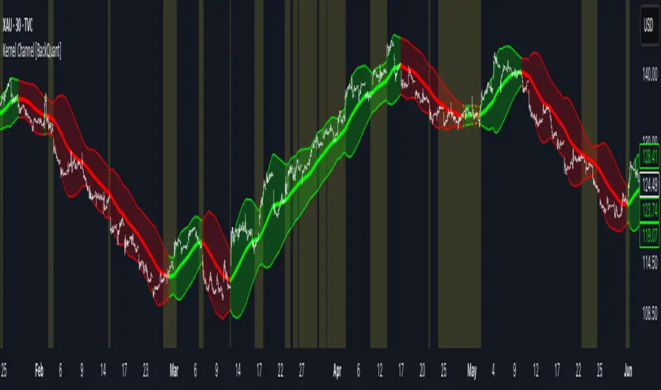
Lorentzian Length Adaptive Moving Average [LLAMA] Adaptation of "Machine Learning: Lorentzian Classification" by
Gradient color by base on work by
LLAMA: A regime-aware adaptive moving average that bends with the market.
Start with a problem traders know:
Traditional moving averages are either too slow (EMA200) or too fast (EMA9)
Adaptive MAs exist, but they often hug price too tightly or smooth too much, failing to balance bias and tactics
LLAMA uses a Lorentzian distance function to adapt its length dynamically. Instead of a fixed smoothing window, it stretches or contracts depending on market conditions. This distortion reduces lag while still providing a clear bias line.
The indicator looks back at recent bars and measures how similar they are using a Lorentzian distance (a log‑scaled absolute difference). It keeps track of the “nearest neighbors” — bars that most resemble the current regime. Each neighbor carries a label (long, short, neutral) based on simple price comparisons. By averaging these labels, LLAMA predicts whether the market is leaning bullish or bearish. That prediction is then mapped into a dynamic length between and .
Bullish bias -> length stretches toward max (smoother, more stable).
Bearish bias -> length contracts toward min (snappier, more reactive).
During breakouts, LLAMA tightens and comes into contact with bars, giving actionable signals. During chop, it stretches to avoid false triggers. It covers both ends of the spectrum (bias and tactics) in one line, something static MA's can't do.
Think of LLAMA as a lens that bends with the market:
Wide lens (max length) for big picture bias.
Narrow lens (min length) for tactical precision.
The "Lorentzian Loop" is the math that decides when to widen or narrow.

Adaptive Momentum Pressure (AMP)🔹 Adaptive Momentum Pressure (AMP)
A hybrid momentum oscillator that adapts to volatility and trend dynamics.
AMP measures the rate of change of price pressure and automatically adjusts its sensitivity based on market volatility.
It reacts faster in trending markets and smooths out noise during consolidation — helping traders identify genuine momentum shifts early while avoiding whipsaws.
🧠 Core Concept
AMP fuses three elements into one adaptive momentum model:
Normalized Momentum (ROC) – captures directional acceleration of price.
Adaptive Smoothing – the smoothing length dynamically contracts when volatility rises and expands when it falls.
Directional Bias – derived from the short-term EMA slope to weight momentum toward the prevailing trend.
Combined, these form a pressure value oscillating between –100 and +100, revealing when momentum expands or fades.
⚙️ How It Works
Calculates a normalized rate of change (ROC) relative to recent volatility.
Adjusts its effective length using the ATR — more volatile periods shorten the lookback for quicker reaction.
Applies a custom EMA that adapts in real time.
Modulates momentum by a normalized EMA slope (“trend bias”).
Produces a smoothed AMP line with a Signal line and crossover markers.
🔍 How to Read It
Green AMP line rising above Signal → Building bullish momentum.
Red AMP line falling below Signal → Fading or bearish momentum.
White Signal line = smoothed confirmation of trend energy.
Green dots = early bullish crossovers.
Red dots = early bearish crossovers.
Typical interpretations:
AMP crossing above 0 from below → early bullish impulse.
AMP peaking near +50–100 and curling down → potential momentum exhaustion.
Crosses below 0 with red pressure → bearish confirmation.
⚡ Advantages
✅ Adaptive across all markets and timeframes
✅ Built-in trend bias filters false signals
✅ Reacts earlier than RSI/MACD while reducing noise
✅ No manual retuning required
🧩 Suggested Use
Combine with structure or volume tools to confirm breakouts.
Works well as a momentum confirmation filter for entries/exits.
Optimal display: separate oscillator pane (not overlay).
Use it responsibly — AMP is an analytical tool, not financial advice.

Volatility-Targeted Momentum Portfolio [BackQuant]Volatility-Targeted Momentum Portfolio
A complete momentum portfolio engine that ranks assets, targets a user-defined volatility, builds long, short, or delta-neutral books, and reports performance with metrics, attribution, Monte Carlo scenarios, allocation pie, and efficiency scatter plots. This description explains the theory and the mechanics so you can configure, validate, and deploy it with intent.
Table of contents
What the script does at a glance
Momentum, what it is, how to know if it is present
Volatility targeting, why and how it is done here
Portfolio construction modes: Long Only, Short Only, Delta Neutral
Regime filter and when the strategy goes to cash
Transaction cost modelling in this script
Backtest metrics and definitions
Performance attribution chart
Monte Carlo simulation
Scatter plot analysis modes
Asset allocation pie chart
Inputs, presets, and deployment checklist
Suggested workflow
1) What the script does at a glance
Pulls a list of up to 15 tickers, computes a simple momentum score on each over a configurable lookback, then volatility-scales their bar-to-bar return stream to a target annualized volatility.
Ranks assets by raw momentum, selects the top 3 and bottom 3, builds positions according to the chosen mode, and gates exposure with a fast regime filter.
Accumulates a portfolio equity curve with risk and performance metrics, optional benchmark buy-and-hold for comparison, and a full alert suite.
Adds visual diagnostics: performance attribution bars, Monte Carlo forward paths, an allocation pie, and scatter plots for risk-return and factor views.
2) Momentum: definition, detection, and validation
Momentum is the tendency of assets that have performed well to continue to perform well, and of underperformers to continue underperforming, over a specific horizon. You operationalize it by selecting a horizon, defining a signal, ranking assets, and trading the leaders versus laggards subject to risk constraints.
Signal choices . Common signals include cumulative return over a lookback window, regression slope on log-price, or normalized rate-of-change. This script uses cumulative return over lookback bars for ranking (variable cr = price/price - 1). It keeps the ranking simple and lets volatility targeting handle risk normalization.
How to know momentum is present .
Leaders and laggards persist across adjacent windows rather than flipping every bar.
Spread between average momentum of leaders and laggards is materially positive in sample.
Cross-sectional dispersion is non-trivial. If everything is flat or highly correlated with no separation, momentum selection will be weak.
Your validation should include a diagnostic that measures whether returns are explained by a momentum regression on the timeseries.
Recommended diagnostic tool . Before running any momentum portfolio, verify that a timeseries exhibits stable directional drift. Use this indicator as a pre-check: It fits a regression to price, exposes slope and goodness-of-fit style context, and helps confirm if there is usable momentum before you force a ranking into a flat regime.
3) Volatility targeting: purpose and implementation here
Purpose . Volatility targeting seeks a more stable risk footprint. High-vol assets get sized down, low-vol assets get sized up, so each contributes more evenly to total risk.
Computation in this script (per asset, rolling):
Return series ret = log(price/price ).
Annualized volatility estimate vol = stdev(ret, lookback) * sqrt(tradingdays).
Leverage multiplier volMult = clamp(targetVol / vol, 0.1, 5.0).
This caps sizing so extremely low-vol assets don’t explode weight and extremely high-vol assets don’t go to zero.
Scaled return stream sr = ret * volMult. This is the per-bar, risk-adjusted building block used in the portfolio combinations.
Interpretation . You are not levering your account on the exchange, you are rescaling the contribution each asset’s daily move has on the modeled equity. In live trading you would reflect this with position sizing or notional exposure.
4) Portfolio construction modes
Cross-sectional ranking . Assets are sorted by cr over the chosen lookback. Top and bottom indices are extracted without ties.
Long Only . Averages the volatility-scaled returns of the top 3 assets: avgRet = mean(sr_top1, sr_top2, sr_top3). Position table shows per-asset leverages and weights proportional to their current volMult.
Short Only . Averages the negative of the volatility-scaled returns of the bottom 3: avgRet = mean(-sr_bot1, -sr_bot2, -sr_bot3). Position table shows short legs.
Delta Neutral . Long the top 3 and short the bottom 3 in equal book sizes. Each side is sized to 50 percent notional internally, with weights within each side proportional to volMult. The return stream mixes the two sides: avgRet = mean(sr_top1,sr_top2,sr_top3, -sr_bot1,-sr_bot2,-sr_bot3).
Notes .
The selection metric is raw momentum, the execution stream is volatility-scaled returns. This separation is deliberate. It avoids letting volatility dominate ranking while still enforcing risk parity at the return contribution stage.
If everything rallies together and dispersion collapses, Long Only may behave like a single beta. Delta Neutral is designed to extract cross-sectional momentum with low net beta.
5) Regime filter
A fast EMA(12) vs EMA(21) filter gates exposure.
Long Only active when EMA12 > EMA21. Otherwise the book is set to cash.
Short Only active when EMA12 < EMA21. Otherwise cash.
Delta Neutral is always active.
This prevents taking long momentum entries during obvious local downtrends and vice versa for shorts. When the filter is false, equity is held flat for that bar.
6) Transaction cost modelling
There are two cost touchpoints in the script.
Per-bar drag . When the regime filter is active, the per-bar return is reduced by fee_rate * avgRet inside netRet = avgRet - (fee_rate * avgRet). This models proportional friction relative to traded impact on that bar.
Turnover-linked fee . The script tracks changes in membership of the top and bottom baskets (top1..top3, bot1..bot3). The intent is to charge fees when composition changes. The template counts changes and scales a fee by change count divided by 6 for the six slots.
Use case: increase fee_rate to reflect taker fees and slippage if you rebalance every bar or trade illiquid assets. Reduce it if you rebalance less often or use maker orders.
Practical advice .
If you rebalance daily, start with 5–20 bps round-trip per switch on liquid futures and adjust per venue.
For crypto perp microcaps, stress higher cost assumptions and add slippage buffers.
If you only rotate on lookback boundaries or at signals, use alert-driven rebalances and lower per-bar drag.
7) Backtest metrics and definitions
The script computes a standard set of portfolio statistics once the start date is reached.
Net Profit percent over the full test.
Max Drawdown percent, tracked from running peaks.
Annualized Mean and Stdev using the chosen trading day count.
Variance is the square of annualized stdev.
Sharpe uses daily mean adjusted by risk-free rate and annualized.
Sortino uses downside stdev only.
Omega ratio of sum of gains to sum of losses.
Gain-to-Pain total gains divided by total losses absolute.
CAGR compounded annual growth from start date to now.
Alpha, Beta versus a user-selected benchmark. Beta from covariance of daily returns, Alpha from CAPM.
Skewness of daily returns.
VaR 95 linear-interpolated 5th percentile of daily returns.
CVaR average of the worst 5 percent of daily returns.
Benchmark Buy-and-Hold equity path for comparison.
8) Performance attribution
Cumulative contribution per asset, adjusted for whether it was held long or short and for its volatility multiplier, aggregated across the backtest. You can filter to winners only or show both sides. The panel is sorted by contribution and includes percent labels.
9) Monte Carlo simulation
The panel draws forward equity paths from either a Normal model parameterized by recent mean and stdev, or non-parametric bootstrap of recent daily returns. You control the sample length, number of simulations, forecast horizon, visibility of individual paths, confidence bands, and a reproducible seed.
Normal uses Box-Muller with your seed. Good for quick, smooth envelopes.
Bootstrap resamples realized returns, preserving fat tails and volatility clustering better than a Gaussian assumption.
Bands show 10th, 25th, 75th, 90th percentiles and the path mean.
10) Scatter plot analysis
Four point-cloud modes, each plotting all assets and a star for the current portfolio position, with quadrant guides and labels.
Risk-Return Efficiency . X is risk proxy from leverage, Y is expected return from annualized momentum. The star shows the current book’s composite.
Momentum vs Volatility . Visualizes whether leaders are also high vol, a cue for turnover and cost expectations.
Beta vs Alpha . X is a beta proxy, Y is risk-adjusted excess return proxy. Useful to see if leaders are just beta.
Leverage vs Momentum . X is volMult, Y is momentum. Shows how volatility targeting is redistributing risk.
11) Asset allocation pie chart
Builds a wheel of current allocations.
Long Only, weights are proportional to each long asset’s current volMult and sum to 100 percent.
Short Only, weights show the short book as positive slices that sum to 100 percent.
Delta Neutral, 50 percent long and 50 percent short books, each side leverage-proportional.
Labels can show asset, percent, and current leverage.
12) Inputs and quick presets
Core
Portfolio Strategy . Long Only, Short Only, Delta Neutral.
Initial Capital . For equity scaling in the panel.
Trading Days/Year . 252 for stocks, 365 for crypto.
Target Volatility . Annualized, drives volMult.
Transaction Fees . Per-bar drag and composition change penalty, see the modelling notes above.
Momentum Lookback . Ranking horizon. Shorter is more reactive, longer is steadier.
Start Date . Ensure every symbol has data back to this date to avoid bias.
Benchmark . Used for alpha, beta, and B&H line.
Diagnostics
Metrics, Equity, B&H, Curve labels, Daily return line, Rolling drawdown fill.
Attribution panel. Toggle winners only to focus on what matters.
Monte Carlo mode with Normal or Bootstrap and confidence bands.
Scatter plot type and styling, labels, and portfolio star.
Pie chart and labels for current allocation.
Presets
Crypto Daily, Long Only . Lookback 25, Target Vol 50 percent, Fees 10 bps, Regime filter on, Metrics and Drawdown on. Monte Carlo Bootstrap with Recent 200 bars for bands.
Crypto Daily, Delta Neutral . Lookback 25, Target Vol 50 percent, Fees 15–25 bps, Regime filter always active for this mode. Use Scatter Risk-Return to monitor efficiency and keep the star near upper left quadrants without drifting rightward.
Equities Daily, Long Only . Lookback 60–120, Target Vol 15–20 percent, Fees 5–10 bps, Regime filter on. Use Benchmark SPX and watch Alpha and Beta to keep the book from becoming index beta.
13) Suggested workflow
Universe sanity check . Pick liquid tickers with stable data. Thin assets distort vol estimates and fees.
Check momentum existence . Run on your timeframe. If slope and fit are weak, widen lookback or avoid that asset or timeframe.
Set risk budget . Choose a target volatility that matches your drawdown tolerance. Higher target increases turnover and cost sensitivity.
Pick mode . Long Only for bull regimes, Short Only for sustained downtrends, Delta Neutral for cross-sectional harvesting when index direction is unclear.
Tune lookback . If leaders rotate too often, lengthen it. If entries lag, shorten it.
Validate cost assumptions . Increase fee_rate and stress Monte Carlo. If the edge vanishes with modest friction, refine selection or lengthen rebalance cadence.
Run attribution . Confirm the strategy’s winners align with intuition and not one unstable outlier.
Use alerts . Enable position change, drawdown, volatility breach, regime, momentum shift, and crash alerts to supervise live runs.
Important implementation details mapped to code
Momentum measure . cr = price / price - 1 per symbol for ranking. Simplicity helps avoid overfitting.
Volatility targeting . vol = stdev(log returns, lookback) * sqrt(tradingdays), volMult = clamp(targetVol / vol, 0.1, 5), sr = ret * volMult.
Selection . Extract indices for top1..top3 and bot1..bot3. The arrays rets, scRets, lev_vals, and ticks_arr track momentum, scaled returns, leverage multipliers, and display tickers respectively.
Regime filter . EMA12 vs EMA21 switch determines if the strategy takes risk for Long or Short modes. Delta Neutral ignores the gate.
Equity update . Equity multiplies by 1 + netRet only when the regime was active in the prior bar. Buy-and-hold benchmark is computed separately for comparison.
Tables . Position tables show current top or bottom assets with leverage and weights. Metric table prints all risk and performance figures.
Visualization panels . Attribution, Monte Carlo, scatter, and pie use the last bars to draw overlays that update as the backtest proceeds.
Final notes
Momentum is a portfolio effect. The edge comes from cross-sectional dispersion, adequate risk normalization, and disciplined turnover control, not from a single best asset call.
Volatility targeting stabilizes path but does not fix selection. Use the momentum regression link above to confirm structure exists before you size into it.
Always test higher lag costs and slippage, then recheck metrics, attribution, and Monte Carlo envelopes. If the edge persists under stress, you have something robust.

VWAP Kalman FilterOverview
This indicator applies Kalman filtering techniques to Volume Weighted Average Price (VWAP) calculations, providing a statistically optimized approach to VWAP analysis. The Kalman filter reduces noise while maintaining responsiveness to genuine price movements, addressing common VWAP limitations in volatile or low-volume conditions.
Technical Implementation
Kalman Filter Mathematics
The indicator implements a state-space model for VWAP estimation:
- Prediction Step: x̂(k|k-1) = x̂(k-1|k-1) + v(k-1)
- Update Step: x̂(k|k) = x̂(k|k-1) + K(k)
- Kalman Gain: K(k) = P(k|k-1) / (P(k|k-1) + R)
Where:
- x̂ = estimated VWAP state
- K = Kalman gain (adaptive weighting factor)
- P = error covariance
- R = measurement noise
- Q = process noise
- v = optional velocity component
Core Components
Dual VWAP System
- Standard VWAP: Traditional volume-weighted calculation
- Kalman-filtered VWAP: Noise-reduced estimation with optional velocity tracking
- Real-time divergence measurement between filtered and unfiltered values
Adaptive Filtering
- Process Noise (Q): Controls adaptation to price changes (0.001-1.0)
- Measurement Noise (R): Determines smoothing intensity (0.01-5.0)
- Optional velocity tracking for momentum-based filtering
Multi-Timeframe Anchoring
- Session, Weekly, Monthly, Quarterly, and Yearly anchor periods
- Automatic Kalman state reset on anchor changes
- Maintains VWAP integrity across timeframes
Features
Visual Components
- Dual VWAP Lines: Compare filtered vs. unfiltered in real-time
- Dynamic Bands: Three-level deviation bands (1σ, 2σ, 3σ)
- Trend Coloring: Automatic color adaptation based on price position
- Cloud Visualization: Highlights divergence between standard and Kalman VWAP
- Signal Markers: Crossover and band-touch indicators
Trading Signals
- VWAP crossover detection with Kalman filtering
- Band touch alerts at multiple standard deviation levels
- Velocity-based momentum confirmation (optional)
- Divergence warnings when filtered/unfiltered values separate
Information Display
- Real-time VWAP values (both standard and filtered)
- Trend direction indicator
- Velocity/momentum reading (when enabled)
- Divergence percentage calculation
- Anchor period display
Input Parameters
VWAP Settings
- Anchor Period: Choose calculation reset period
- Band Multipliers: Customize deviation band distances
- Display Options: Toggle standard VWAP and bands
Kalman Parameters
- Length: Base period for calculations (5-200)
- Process Noise (Q: Higher values increase responsiveness
- Measurement Noise (R): Higher values increase smoothing
- Velocity Tracking: Enable momentum-based filtering
Visual Controls
- Toggle filtered/unfiltered VWAP display
- Band visibility options
- Signal markers on/off
- Cloud fill between VWAPs
- Bar coloring by trend
Use Cases
Noise Reduction
Particularly effective during:
- Low volume periods (pre-market, lunch hours)
- Volatile market conditions
- Fast-moving markets where standard VWAP whipsaws
Trend Identification
- Cleaner trend signals with reduced false crosses
- Earlier trend detection through velocity component
- Confirmation through divergence analysis
Support/Resistance
- Filtered VWAP provides more stable S/R levels
- Bands adapt to filtered values for better zone identification
- Reduced false breakout signals
Technical Advantages
1. Optimal Estimation: Mathematically optimal under Gaussian noise assumptions
2. Adaptive Response: Self-adjusting to market conditions
3. Predictive Element: Velocity component provides forward-looking insight
4. Noise Immunity: Superior noise rejection vs. simple moving average smoothing
Limitations
- Assumes linear price dynamics
- Requires parameter optimization for different instruments
- May lag during sudden volatility regime changes
- Not suitable as standalone trading system
Mathematical Background
Based on control systems theory, the Kalman filter provides recursive Bayesian estimation originally developed for aerospace applications. This implementation adapts the algorithm specifically for financial time series, maintaining VWAP's volume-weighted properties while adding statistical filtering.
Comparison with Standard VWAP
Standard VWAP Issues Addressed:
- Choppy behavior in low volume
- Whipsaws around VWAP line
- Lag in trend identification
- Noise in deviation bands
Kalman VWAP Benefits:
- Smooth yet responsive line
- Fewer false signals
- Optional momentum tracking
- Statistically optimized filtering
Alert Conditions
The indicator includes several pre-configured alert conditions:
- Bullish/Bearish VWAP crosses
- Upper/Lower band touches
- High divergence warnings
- Velocity shifts (if enabled)
---
This open-source indicator is provided as-is for educational and trading purposes. No guarantees are made regarding trading performance. Users should conduct their own testing and validation before using in live trading.

Dynamic Fractal Flow [Alpha Extract]An advanced momentum oscillator that combines fractal market structure analysis with adaptive volatility weighting and multi-derivative calculus to identify high-probability trend reversals and continuation patterns. Utilizing sophisticated noise filtering through choppiness indexing and efficiency ratio analysis, this indicator delivers entries that adapt to changing market regimes while reducing false signals during consolidation via multi-layer confirmation centered on acceleration analysis, statistical band context, and dynamic omega weighting—without any divergence detection.
🔶 Fractal-Based Market Structure Detection
Employs Williams Fractal methodology to identify pivotal market highs and lows, calculating normalized price position within the established fractal range to generate oscillator signals based on structural positioning. The system tracks fractal points dynamically and computes relative positioning with ATR fallback protection, ensuring continuous signal generation even during extended trending periods without fractal formation.
🔶 Dynamic Omega Weighting System
Implements an adaptive weighting algorithm that adjusts signal emphasis based on real-time volatility conditions and volume strength, calculating dynamic omega coefficients ranging from 0.3 to 0.9. The system applies heavier weighting to recent price action during high-conviction moves while reducing sensitivity during low-volume environments, mitigating lag inherent in fixed-period calculations through volatility normalization and volume-strength integration.
🔶 Cascading Robustness Filtering
Features up to five stages of progressive EMA smoothing with user-adjustable robustness steps, each layer systematically filtering microstructure noise while preserving essential trend information. Smoothing periods scale with the chosen fractal length and robustness steps using a fixed smoothing multiplier for consistent, predictable behavior.
🔶 Adaptive Noise Suppression Engine
Integrates dual-component noise filtering combining Choppiness Index calculation with Kaufman’s Efficiency Ratio to detect ranging versus trending market conditions. The system applies dynamic damping that maintains full signal strength during trending environments while suppressing signals during choppy consolidation, aligning output with the prevailing regime.
🔶 Acceleration and Jerk Analysis Framework
Calculates second-derivative acceleration and third-derivative jerk to identify explosive momentum shifts before they fully materialize on traditional indicators. Detects bullish acceleration when both acceleration and jerk turn positive in negative oscillator territory, and bearish acceleration when both turn negative in positive territory, providing early entry signals for high-velocity trend initiation phases.
🔶 Multi-Layer Signal Generation Architecture
Combines three primary signal types with hierarchical validation: acceleration signals, band crossover entries, and threshold momentum signals. Each signal category includes momentum confirmation, trend-state validation, and statistical band context; signals are further conditioned by band squeeze detection to avoid low-probability entries during compression phases. Divergence is intentionally excluded for a purely structure- and momentum-driven approach.
🔶 Dynamic Statistical Band System
Utilizes Bollinger-style standard deviation bands with configurable multiplier and length to create adaptive threshold zones that expand during volatile periods and contract during consolidation. Includes band squeeze detection to identify compression phases that typically precede expansion, with signal suppression during squeezes to prevent premature entries.
🔶 Gradient Color Visualization System
Features color gradient mapping that dynamically adjusts line intensity based on signal strength, transitioning from neutral gray to progressively intense bullish or bearish colors as conviction increases. Includes gradient fills between the signal line and zero with transparency scaling based on oscillator intensity for immediate visual confirmation of trend strength and directional bias.
All analysis provided by Alpha Extract is for educational and informational purposes only. The information and publications are not meant to be, and do not constitute, financial, investment, trading, or other types of advice or recommendations.

Adaptive Trend SelectorThe Adaptive Trend Selector is a comprehensive trend-following tool designed to automatically identify the optimal moving average crossover strategy. It features adjustable parameters and an integrated backtester that delivers institutional-grade insights into the recommended strategy. The model continuously adapts to new data in real time by evaluating multiple moving average combinations, determining the best performing lengths, and presenting the backtest results in a clear, color-coded table that benchmarks performance against the buy-and-hold strategy.
At its core, the model systematically backtests a wide range of moving average combinations to identify the configuration that maximizes the selected optimization metric. Users can choose to optimize for absolute returns or risk-adjusted returns using the Sharpe, Sortino, or Calmar ratios. Alternatively, users can enable manual optimization to test custom fast and slow moving average lengths and view the corresponding backtest results. The label displays the Compounded Annual Growth Rate (CAGR) of the strategy, with the buy-and-hold CAGR in parentheses for comparison. The table presents the backtest results based on the fast and slow lengths displayed at the top:
Sharpe = CAGR per unit of standard deviation.
Sortino = CAGR per unit of downside deviation.
Calmar = CAGR relative to maximum drawdown.
Max DD = Largest peak-to-trough decline in value.
Beta (β) = Return sensitivity relative to buy-and-hold.
Alpha (α) = Excess annualized risk-adjusted returns.
Win Rate = Ratio of profitable trades to total trades.
Profit Factor = Total gross profit per unit of losses.
Expectancy = Average expected return per trade.
Trades/Year = Average number of trades per year.
This indicator is designed with flexibility in mind, enabling users to specify the start date of the backtesting period and the preferred moving average strategy. Supported strategies include the Exponential Moving Average (EMA), Simple Moving Average (SMA), Wilder’s Moving Average (RMA), Weighted Moving Average (WMA), and Volume-Weighted Moving Average (VWMA). To minimize overfitting, users can define constraints such as a minimum and maximum number of trades per year, as well as an optional optimization margin that prioritizes longer, more robust combinations by requiring shorter-length strategies to exceed this threshold. The table follows an intuitive color logic that enables quick performance comparison against buy-and-hold (B&H):
Sharpe = Green indicates better than B&H, while red indicates worse.
Sortino = Green indicates better than B&H, while red indicates worse.
Calmar = Green indicates better than B&H, while red indicates worse.
Max DD = Green indicates better than B&H, while red indicates worse.
Beta (β) = Green indicates better than B&H, while red indicates worse.
Alpha (α) = Green indicates above 0%, while red indicates below 0%.
Win Rate = Green indicates above 50%, while red indicates below 50%.
Profit Factor = Green indicates above 2, while red indicates below 1.
Expectancy = Green indicates above 0%, while red indicates below 0%.
In summary, the Adaptive Trend Selector is a powerful tool designed to help investors make data-driven decisions when selecting moving average crossover strategies. By optimizing for risk-adjusted returns, investors can confidently identify the best lengths using institutional-grade metrics. While results are based on the selected historical period, users should be mindful of potential overfitting, as past results may not persist under future market conditions. Since the model recalibrates to incorporate new data, the recommended lengths may evolve over time.
