Breakout Targets [AlgoAlpha]🟠 OVERVIEW
This script identifies consolidation zones and provides automated breakout targets with risk management levels. It focuses on finding periods where price action compresses and then tracks the subsequent breakout from these ranges. When a price breakout is confirmed, the script automatically projects three take-profit (TP) levels and a stop-loss (SL) based on current market volatility. This helps traders move from identifying a range to executing a trade with predefined exit points without manual calculation.
🟠 CONCEPTS
The script uses a relationship between Weighted Moving Averages (WMA) and Exponential Moving Averages (EMA) of price ranges to detect consolidation. When these moving averages cross, it triggers the detection of recent pivot highs and lows to draw a visual "box" or channel. This channel represents the current trading range. Once price closes outside this box, the script uses the Average True Range (ATR) to determine the volatility-adjusted distance for the stop loss. The take-profit levels are then calculated as multiples of this risk distance, ensuring a consistent reward-to-risk approach.
🟠 FEATURES
Dynamic box drawing that highlights potential supply and demand zones within the range.
Real-time breakout signals with bullish (green) and bearish (red) markers.
Automated trade projection including Entry, SL, and three TP levels.
Integrated alert system for breakouts and hits on any profit or loss target.
🟠 USAGE
Setup : Add the script to your chart and adjust the "Range Detection Period." A higher period will find larger, more significant ranges, while a lower period will find smaller, short-term consolidation zones.
Read the chart : Look for the grey boxes on your chart; these represent areas where the market is "coiling." A green arrow label indicates a bullish breakout from the top of the box, while a red arrow indicates a bearish breakout from the bottom. Once a breakout occurs, follow the projected horizontal levels for your trade management.
Settings that matter : The Stop Loss ATR Multiplier is the most critical setting for risk; increasing it will give the trade more room to breathe but will also push your TP levels further away. The Prevent Overlap toggle is useful for keeping the chart clean by ensuring the script doesn't draw new boxes until the current range has been resolved.
Meanreversion

Quantum Mean Reversion Oscillator[Pineify]Quantum Mean Reversion Oscillator - Statistical Z-Score Based Trading Signals
The Quantum Mean Reversion Oscillator (QMR) is a statistically-driven momentum indicator designed to identify high-probability mean reversion opportunities in any market. Built on the foundation of Z-score analysis, this oscillator measures how far price has deviated from its statistical mean, expressed in standard deviations. When price stretches too far from equilibrium, it tends to snap back—this indicator captures those precise moments.
Key Features
Z-Score based oscillator measuring price deviation from dynamic mean
Adaptive EMA-based mean calculation for responsive trend detection
Customizable standard deviation multiplier for volatility adjustment
Built-in smoothing to filter market noise and reduce false signals
Visual gradient glow effect showing momentum intensity
Clear overbought/oversold threshold levels at +2.0 and -2.0
Automatic buy and sell signal generation on mean reversion events
Pre-configured alert conditions for automated trading workflows
How It Works
The indicator employs a three-step calculation process rooted in statistical analysis:
Dynamic Mean Calculation: Rather than using a simple moving average, the oscillator uses an Exponential Moving Average (EMA) as the basis. This makes the mean more responsive to recent price action while still maintaining statistical validity.
Z-Score Computation: The core of this indicator is the Z-score formula: (Price - Mean) / Standard Deviation. This transforms raw price data into a normalized scale where values represent how many standard deviations price has moved from its mean. A reading of +2.0 means price is two standard deviations above average—a statistically significant extreme.
Noise Reduction: The raw Z-score is smoothed using a Simple Moving Average to eliminate whipsaws and provide cleaner, more actionable signals.
Trading Ideas and Insights
Mean reversion is one of the most fundamental concepts in quantitative trading. Markets tend to oscillate around fair value, and extreme deviations often precede reversals. The QMR Oscillator quantifies this behavior:
When the oscillator exceeds +2.0, price is statistically overbought—approximately 95% of price action occurs below this level under normal distribution
When the oscillator drops below -2.0, price is statistically oversold—a zone where buying pressure typically emerges
The crossback signals (crossing back inside from extremes) indicate the reversion has begun, providing entry timing
This approach works particularly well in ranging markets and can identify exhaustion points in trending markets where pullbacks are likely.
How Multiple Indicators Work Together
The QMR Oscillator integrates three complementary statistical concepts into a unified framework:
EMA for Mean: Provides a responsive baseline that adapts to changing market conditions faster than traditional SMA, ensuring the "fair value" reference point stays relevant.
Standard Deviation for Volatility: Automatically adjusts the oscillator's sensitivity based on current market volatility. During high volatility, larger price moves are required to reach extreme readings, preventing false signals.
SMA Smoothing: Applied as a final filter to remove noise without introducing significant lag, balancing responsiveness with reliability.
These three components work synergistically—the EMA tracks the trend, standard deviation normalizes for volatility, and smoothing ensures signal quality.
Unique Aspects
Statistical Foundation: Unlike arbitrary oscillator boundaries, the +/-2.0 levels have statistical meaning—representing approximately 2 standard deviations from the mean
Visual Gradient System: The glow effect intensifies as price moves further from equilibrium, providing intuitive visual feedback on momentum strength
Adaptive Sensitivity: The deviation multiplier allows traders to adjust how extreme price must move before triggering signals, accommodating different trading styles and market conditions
How to Use
Add the indicator to your chart and observe the oscillator's position relative to the zero line and threshold levels
Look for buy signals (B markers) when the oscillator crosses back above -2.0 from oversold territory
Look for sell signals (S markers) when the oscillator crosses back below +2.0 from overbought territory
Use the gradient glow intensity to gauge momentum strength—brighter colors indicate more extreme conditions
Set up alerts using the built-in alert conditions for automated notifications
Customization
Mean Lookback (default: 20): Controls the EMA period for mean calculation. Shorter periods increase sensitivity; longer periods provide smoother readings
Deviation Multiplier (default: 2.0): Adjusts how many standard deviations define the bands. Higher values require more extreme moves for signals
Smoothing (default: 3): Controls noise filtering. Increase for smoother signals in choppy markets
Bullish/Bearish Glow Colors: Customize the visual appearance to match your chart theme
Show Reversion Signals: Toggle buy/sell markers on or off
Conclusion
The Quantum Mean Reversion Oscillator provides traders with a statistically rigorous tool for identifying mean reversion opportunities. By combining Z-score analysis with adaptive volatility measurement and intelligent smoothing, it offers a systematic approach to finding high-probability reversal points. Whether used as a standalone indicator or as confirmation for other analysis methods, the QMR Oscillator brings quantitative precision to mean reversion trading strategies.

Adaptive RSIAdaptive RSI
Adaptive RSI is an enhanced version of the classic Relative Strength Index designed to automatically adjust its behavior to changing market conditions. The indicator can operate both as a mean-reversion oscillator and as a trend-following momentum tool, allowing traders to detect high/low value zones while also capturing directional moves.
Unlike the traditional RSI, which uses a fixed smoothing method, Adaptive RSI dynamically changes its calculation speed depending on market activity. This helps reduce false signals in slow or choppy markets while allowing faster responses during strong moves.
🔍 Concept & Idea
The goal behind Adaptive RSI is to make RSI responsive when opportunities appear and more conservative during uncertain or low-activity environments.
By automatically adjusting its internal smoothing and reaction speed, the indicator attempts to balance:
• Early entries during strong market moves
• Reduced noise during consolidation
• Mean-reversion opportunities in ranging markets
• Momentum confirmation in trending markets
This adaptive behavior makes the oscillator more versatile across multiple market conditions.
⚙️ How It Works
The indicator evaluates market activity using three drivers:
• True Range (volatility)
• Volume activity
• Rate of price change
Users can define which of these factors has priority. The script then checks up to three conditions; the more conditions that are satisfied, the faster and more responsive the RSI calculation becomes.
This creates multiple internal speed tiers ranging from smooth and conservative to highly responsive.
After the adaptive RSI is calculated, an additional adaptive smoothing layer is applied using the same logic, improving signal clarity while preserving responsiveness.
An optional feature allows the RSI to use a special Rate-of-Change weighted price source. This feature is more advanced and mainly intended for users who understand how weighted price construction affects oscillators.
A divergence measure between the base RSI and the smoothed Adaptive RSI is also plotted to help visualize shifts in momentum strength.
⚙️ Key Features
• Adaptive RSI calculation speed
• Works for both trend-following and mean-reversion approaches
• Adjustable long and short signal thresholds
• Overbought and oversold zone highlighting
• Divergence histogram between RSI and adaptive smoothing
• Trend-based coloring and visual signal markers
• Optional ROC-weighted source for advanced users
🧩 Inputs Overview
• RSI calculation length and smoothing length
• Price source selection or optional special weighted source
• Speed tier selection (slow, medium, fast behavior)
• Activity priority order (volatility, volume, momentum)
• Long/short and overbought/oversold thresholds
📌 Usage Notes
• Can be used both for trend continuation and mean-reversion strategies.
• Adaptive logic helps reduce noise during sideways markets.
• Strong moves may cause faster RSI transitions due to adaptive speed selection.
• Signals may update intrabar on lower timeframes.
• Works best when combined with risk management and confirmation tools.
• No indicator is perfect; always test before live use.
This script is intended for analytical purposes only and does not provide financial advice.

SPY Quant ML + Session Filter Strategy [CocoChoco]S&P 500 Quant: Machine Learning & Mean Reversion (Session-Filtered)
Overview
This is a professional-grade quantitative strategy designed specifically for the S&P 500. It combines classical statistical mean reversion (Z-Score) with a modern Machine Learning filter and rigorous institutional-grade risk management.
The strategy is optimized for traders who prioritize high win rates and capital preservation, specifically avoiding the "gap risk" associated with holding positions overnight.
Core Methodology
1. Statistical Entry (The Z-Score Engine)
The strategy identifies "oversold" conditions in a bullish context. It calculates the Z-Score of the price relative to its 20-period Mean (SMA). By default, it looks for a -1.2 Standard Deviation extension, signaling a high-probability "dip" ripe for a snap-back to the mean.
2. Trend & ML Filters
To avoid "catching a falling knife," the strategy uses two layers of confirmation:
Trend Filter: Only takes Long positions when the price is above the 200-period SMA, ensuring we only buy dips in a confirmed uptrend.
ML Correlation Filter: A Machine Learning-inspired module that analyzes the correlation between RSI and Volatility (ATR). It only permits entries when market internal dynamics suggest a reversal is technically "healthy."
3. Institutional Risk Management
This script is built for "safety-first" automation:
Hard Stop Loss: Fixed at 1.5% to protect against sudden market shocks.
Active Trailing: A dual-trigger trailing stop. It activates once the price touches the 20 SMA (The Mean) OR once a trade reaches a 0.50% profit threshold. This ensures near-winners are protected and large runners are captured.
Intraday Circuit Breaker: Includes a Max Daily Drawdown (2%) limit. If hit, the script automatically closes losing positions and halts trading for the day, while allowing winning positions to continue.
Key Features
Session-Specific: Tailored for the US Trading Session (UTC/NY times).
Zero Overnight Risk: Automatically flattens all positions before the market close (16:00 NY Time).
Holiday Intelligence: Hard-coded logic for US Market Holidays and Early Closes (2026–2028), ensuring the bot doesn't get stuck in illiquid holiday markets.
Hourly Entry Cap: Limits entries to one per hour to prevent over-concentration during a single price leg.
How to Use
Timeframe: I suggest you use it on the 5-minute or 1-hour timeframe for optimal results.
Instrument: Designed for the S&P 500, but highly effective on SPY, IVV, and ES (Futures).
Pyramiding: Designed to handle up to 3 concurrent positions, allowing the strategy to scale into a move as the Z-Score deepens.
Automation Ready
This script is fully compatible with webhook-based automation tools. All signals (Entry, SL, Trail, Market Close, and Daily Limit) are clearly labeled in the Alert comments for seamless execution. I haven't tasted it though. This is not financial advice. Please perform your own tests and manage your risk.
Disclaimer
Past performance does not guarantee future results. This script is a tool for quantitative analysis and should be used as part of a broader diversified trading plan.

Tanh Clamped Momentum Oscillator [Alpha Extract]A sophisticated momentum measurement system that combines dual EMA trend analysis with volatility-weighted pressure calculations, applying hyperbolic tangent normalization for bounded oscillator output with adaptive signal generation. Utilizing ATR-based volatility regime detection and candle pressure metrics, this indicator delivers institutional-grade momentum assessment with multi-tiered band structure and pulse-based envelope visualization. The system's tanh clamping methodology prevents extreme outliers while maintaining sensitivity to genuine momentum shifts, combined with histogram divergence detection and comprehensive alert framework for high-probability reversal and continuation signals.
🔶 Advanced Dual-Component Momentum Engine
Implements hybrid calculation combining EMA trend differential with candle pressure analysis, weighted by volatility regime assessment for context-aware momentum measurement. The system calculates fast and slow EMA difference normalized by ATR, measures intrabar pressure as close-open relative to range, applies volatility-based weighting between trend and pressure components, and produces composite raw momentum capturing both directional bias and internal candle dynamics.
// Core Momentum Framework
EMA_Fast = ta.ema(src, Fast_Length)
EMA_Slow = ta.ema(src, Slow_Length)
Trend = EMA_Fast - EMA_Slow
// Volatility Regime Detection
ATR_Short = ta.atr(ATR_Length)
ATR_Long = ta.atr(ATR_Length * 2)
Vol_Ratio = ATR_Short / ATR_Long
Vol_Weight = clamp((Vol_Ratio - 0.5) / 1.0, 0, 1)
// Pressure Component
Pressure = (close - open) / (high - low)
// Composite Momentum
Raw = Trend_Normalized * Vol_Weight + Pressure_Scaled * (1 - Vol_Weight)
🔶 Hyperbolic Tangent Normalization Framework
Features sophisticated tanh transformation that clamps raw momentum into bounded range while preserving proportional sensitivity across varying market conditions. The system applies safe exponential calculations with input capping to prevent overflow, computes hyperbolic tangent to compress extreme values while maintaining linearity near zero, and scales output by configurable factor creating oscillator with enhanced dynamic range and reduced outlier distortion.
// Tanh Clamping Logic
tanh(x) =>
x_clamped = clamp(x, -5.0, 5.0)
e = exp(2.0 * x_clamped)
(e - 1.0) / (e + 1.0)
Oscillator = tanh(Smoothed_Momentum / Clamp_Factor) * Scale
🔶 Volatility Regime Weighting System
Implements intelligent volatility assessment comparing short-term and long-term ATR to determine market regime, dynamically adjusting weight between trend and pressure components. The system calculates ATR ratio, normalizes to 0-1 range, and uses this weight factor to emphasize trend component during high-volatility regimes and pressure component during low-volatility consolidations, creating adaptive momentum sensitive to market microstructure.
🔶 Multi-Tiered Band Architecture
Provides comprehensive threshold structure with soft, hard, and maximum bands marking progressive momentum extremes for graduated overbought/oversold assessment. The system establishes configurable levels at soft zones (initial caution), hard zones (strong extreme), and maximum zones (critical overextension) with visual differentiation through line styles and background highlighting, enabling nuanced interpretation beyond binary extreme detection.
🔶 Pulse Envelope Visualization
Features dynamic envelope bands calculated from exponential moving average of absolute oscillator value, creating adaptive boundary that expands during momentum acceleration and contracts during deceleration. The system applies configurable length and width multiplier to pulse calculation, fills area between positive and negative pulse bounds with gradient coloring matching oscillator direction, providing visual context for momentum magnitude relative to recent activity.
🔶 Signal Line Integration Framework
Implements dual-mode signal line supporting both EMA and SMA smoothing of primary oscillator for crossover-based swing detection. The system calculates configurable-length moving average, generates histogram differential between oscillator and signal, applies additional smoothing to histogram for noise reduction, and uses crossovers/crossunders as momentum swing indicators distinguishing bullish and bearish momentum shifts.
🔶 Histogram Divergence Display
Creates column-style histogram visualization showing oscillator-signal differential with intensity-based coloring reflecting momentum acceleration or deceleration. The system plots histogram bars in bright colors when expanding (accelerating momentum) and faded colors when contracting (decelerating momentum), enabling instant visual identification of momentum divergences and convergences without numerical analysis.
🔶 Advanced Reversion Signal Logic
Generates overbought/oversold signals requiring both signal line crossover and extreme threshold breach for high-conviction reversal identification. The system triggers oversold when oscillator crosses above signal while below negative reversion level, triggers overbought when crossing below signal while above positive reversion level, and plots small circle markers at signal locations for clear visual confirmation of setup conditions.
🔶 Comprehensive Alert Framework
Provides six distinct alert conditions covering overbought/oversold reversions, midline trend changes, and oscillator-signal swings with configurable notification preferences. The system includes alerts for extreme reversions (OB/OS), zero-line crossovers (trend changes), and signal line crossovers (momentum swings), enabling traders to monitor critical oscillator events across multiple signal types without constant chart observation.
🔶 Adaptive Bar Coloring System
Implements four coloring modes including midline cross (trend direction), extremities (threshold breach), reversions (OB/OS signals), and slope (oscillator vs signal) for customizable visual integration. The system applies selected color scheme to candles providing chart-level momentum feedback, with option to disable coloring for minimal visual interference while maintaining oscillator pane analysis.
🔶 Performance Optimization Architecture
Utilizes efficient tanh calculation with safe clamping, streamlined EMA computations, and optimized ATR ratio processing for smooth real-time updates. The system includes intelligent null handling, minimal recalculation overhead through smart smoothing application, and configurable display toggles allowing users to disable unused visual elements for enhanced performance during extended historical analysis.
🔶 Why Choose Tanh-Clamped Momentum Oscillator ?
This indicator delivers sophisticated momentum analysis through hybrid trend-pressure calculation with volatility-adaptive weighting and hyperbolic tangent normalization. Unlike traditional momentum oscillators susceptible to extreme outlier distortion, the tanh clamping ensures bounded output while preserving sensitivity to genuine momentum shifts. The system's dual-component architecture combining directional trend with intrabar pressure, weighted by volatility regime assessment, creates context-aware momentum measurement that adapts to market microstructure. The multi-tiered band structure, pulse envelope visualization, and comprehensive signal framework make it essential for traders seeking nuanced momentum analysis with graduated extreme detection and high-probability reversal signals across cryptocurrency, forex, and equity markets.

Mean Reversion [SIMI]This mean reversion indicator identifies extreme price deviations from the mean, providing high-probability reversal signals. Designed for confluence-based trading, it works best when combined with complementary indicators such as VWAP, price action, and volume analysis.
📊 Core Features
Signal Types
Prime Signals (Bright Green/Red Dots): Extreme reversions usually beyond ±1.5 SD - highest probability setups (you can customise this zone!)
Regular Signals (Dark Green/Red Dots): Standard reversions - moderate probability
Leader Line (Pink Dotted): Early warning indicator for potential reversals
Histogram Weakness: Momentum divergence signals
Normalisation Methods:
Institutional Hybrid (Z-ATR) (Recommended): Volatility-adjusted Z-score - adapts to changing market conditions
Percentile Ranking: Statistical ranking - excellent for ranging markets
PPO + ATR Hybrid: Percentage-based with volatility adjustment
Efficiency Ratio: Trend-strength weighted
ATR: Pure volatility-based
None: Raw Z-score
⚙️ Quick Setup Guide
1. Institutional Presets
Pre-configured parameter sets optimised for different timeframes:
5M Day Trading (5/21/5): Intraday scalping
1H Options Trading (6/24/5): Options-focused setups
1D Monthly Cycle (5/20/5): Swing trading
2. Signal Filtering
Prime Thresholds: Adjust ±1.5 SD to control signal quality (tighter = fewer, higher quality, adjust this zone per asset traded)
Dot Filters: Fine-tune entry zones (-0.03/+0.03 default - this ignores noisy signals near Zero line)
Volume Filter: Enable to require volume confirmation (1.4x average recommended, but fine tune yourself)
3. Advanced Filters
Dynamic SD Thresholds: Auto-adjusts for volatility regimes (tighter in low vol, wider in high vol)
Time of Day Filter: Avoids first 30 minutes, last 15 minutes, and lunch hour (11:30-13:00 EST)
💡 Trading Strategy Recommendations
Optimal Usage
This indicator is not intended as a standalone system. Use it for confluence alongside:
VWAP (institutional positioning)
Price action (support/resistance)
Options flow (institutional direction)
Volume analysis (conviction confirmation)
Signal Interpretation
Prime Signals: Wait for these for highest-probability entries - mean reversion may take hours to days
Manual Entries: Don't wait for dots - trade the ±2 SD zones directly using your own confirmation
Options Strategy: Prime sell signals at +2 SD make excellent short call setups; prime buy signals at -2 SD for long calls
Timeframe Guidance
Lower Timeframes (1M-5M): Higher noise - require additional confluence
Higher Timeframes (1H-1D): More reliable signals - suitable for options and swing trades
Best Results: Multi-timeframe analysis (check 1H and 4H alignment on 5M entries)
🔔 Alert System
Master Alert
Enable customisable alerts via the Master Alert System:
Toggle individual signal types (Prime Buy/Sell, SD Crosses, Leader, Histogram)
Receives bespoke messages with ticker, timeframe, and price
One alert condition handles all selected signals
Individual Alerts
Separate alert conditions available for Prime and Regular signals if preferred.
📈 Backtesting Notes
Important: Backtest results are date-sensitive and should not be the primary focus. Instead:
Dial in settings visually on your chosen asset
Aim for signals near actual tops and bottoms
Test different normalisation methods for your specific instrument
Optimise for signal quality, not backtest ROI
Asset Testing: Primarily developed using SPY, QQQ, and IWM as main assets to trade. Other instruments may require parameter adjustment - mess around!
Backtest Engine
Entry/Exit modes (All Signals, Prime Only, Early Signals)
Position sizing (percentage-based)
Slippage and fill method (candle close recommended)
Date range selection
⚠️ Best Practices
Always use confluence - never trade on MR signals alone
Start with Institutional Hybrid normalisation - most adaptive to market conditions
Focus on Prime signals for quality over quantity
Test on your specific asset - optimal settings vary by instrument
Longer timeframes = higher reliability - 1H+ for best results
Enable Time Filter on intraday charts to avoid volatile periods
Use Dynamic SD in highly volatile markets (earnings, FOMC, etc.)
🛠️ Troubleshooting
Too many signals: Increase Prime Thresholds or enable Volume Filter
Too few signals: Decrease Prime Thresholds or reduce Dot Filters
False signals: Enable Time of Day Filter and Dynamic SD
Signals don't align with tops/bottoms: Try different normalisation method
📝 Feedback & Development
Bug Reports: Please report any issues via TradingView comments or direct message.
Strategy Sharing: I'd love to hear how you're using this indicator and what strategies you've developed.
Open Source: Feel free to fork and modify this indicator. If you create an improved version, please share it with the community!
🙏 Acknowledgements
Developed through AI-assisted collaboration.
Special thanks to Lazy Bear for his open source MACD histogram (volume based).
Open source forever - use freely, modify, and share.
Happy Trading!
Remember: Past performance does not guarantee future results. Always manage risk appropriately.
Pandas rock \m/

Breaker Blocks Signals [AlgoAlpha]🟠 OVERVIEW
This script automates the detection of Breaker Blocks, a popular smart money concept used to identify high-probability reversal zones. It monitors price action for aggressive impulses—measured through a normalized Z-Score—to identify Orderblocks. When these blocks are "broken" or invalidated by price moving through them, they transform into Breaker Blocks. These zones act as "flipped" support or resistance, offering traders specific areas to look for retests and trend continuations. By handling the complex management of zone life-cycles and mitigation, this script provides a clean, real-time map of institutional supply and demand shifts.
🟠 CONCEPTS
The indicator relies on the relationship between price momentum and structural invalidation. It first identifies "impulsive" candles by calculating a Z-Score of price distance covered over a specific window. A Z-Score above 4 marks an "Algorithmically Significant" move. When such a move occurs, the script identifies the last opposite-colored candle (the Orderblock) and draws a gray zone. The transformation happens when price closes entirely through one of these gray zones. This "mitigation" is what triggers the creation of a Breaker Block: an old bearish supply zone becomes a bullish demand zone, and vice versa. This transition reflects a shift in market regime where previous trapped participants are forced to exit, often leading to price rejections at these newly formed levels.
🟠 FEATURES
Automated Breaker Transformation : Instantly flips mitigated Orderblocks into colored Breaker Blocks (Bullish/Bearish).
Rejection Markers : Small arrow icons appear when price enters a Breaker Block and shows signs of respect/reversal.
Comprehensive Alerts : Notifications for both the formation of new breakers and real-time price rejections.
🟠 USAGE
Setup : Add the script to your chart. It is effective on most timeframes, but many traders prefer the 15m or 1h for intraday structure. Use the "Z-Score Window" to adjust sensitivity; 100 is standard, but lower values (e.g., 50) will find more frequent, smaller impulses.
Read the chart : Gray boxes are "Pending" blocks. If price closes above a gray bearish box, it turns into a Bullish Breaker (Green). If price closes below a gray bullish box, it turns into a Bearish Breaker (Red). Look for price to return to these colored zones; the "▲" and "▼" symbols indicate the script has detected a rejection from that level.
Settings that matter : Prevent Overlap is useful for avoiding "cluttered" zones in ranging markets. Max Box Age is critical; it ensures that very old, irrelevant zones are removed from your chart after a set number of bars, keeping your technical analysis current and focused on recent price action.

Smart RSI Candles [DotGain]Smart RSI Candles – Description
Smart RSI Candles is a minimalist yet powerful overlay indicator that visualizes RSI conditions directly on price candles. Instead of plotting a separate RSI oscillator, this tool colors the chart bars based on customizable RSI threshold levels, allowing traders to instantly identify overbought and oversold regimes within the price action itself.
The indicator is built on the classic Wilder RSI and supports up to three upper (overbought) and three lower (oversold) levels. Each level can be individually enabled or disabled, making the indicator fully modular and adaptable to different trading styles and market conditions.
Key Features
RSI-based candle coloring (no separate panel required)
Up to 6 customizable RSI levels
Individual On/Off toggle for each level
Extreme conditions highlighted in blue
Works on any market and timeframe
Clean, non-intrusive visual design
Color Logic
Overbought (Upper Levels)
Level 1: Light green → mild overbought
Level 2: Dark green → strong overbought
Level 3: Blue → extreme overbought
Oversold (Lower Levels)
Level 1: Light red → mild oversold
Level 2: Dark red → strong oversold
Level 3: Blue → extreme oversold
Neutral RSI values keep the original candle color.
How to Use
Use upper levels to identify potential exhaustion in bullish moves.
Use lower levels to spot potential panic or capitulation zones.
Combine with trend analysis, support/resistance, or volume for confirmations.
Disable specific levels to create conservative or aggressive RSI regimes.
Use Cases
Mean reversion strategies
Momentum exhaustion detection
Visual risk regime mapping
Multi-timeframe RSI context
Smart RSI Candles is designed for traders who want RSI information integrated directly into price, without clutter — fast, intuitive, and highly customizable.
Have fun :)
Disclaimer
This Smart RSI Candles indicator is provided for informational and educational purposes only. It does not, and should not be construed as, financial, investment, or trading advice.
This indicator is an independent implementation of a Relative Strength Index (RSI) based visualization tool and is not affiliated with, or endorsed by, any third-party trading systems, strategies, or trademarked methodologies. The colored candles displayed by this indicator are generated by a predefined set of algorithmic conditions based on RSI threshold levels. They do not constitute a direct recommendation to buy or sell any financial instrument.
All trading and investing in financial markets involves a substantial risk of loss. You may lose part or all of your invested capital. Past performance does not guarantee future results. This indicator highlights potential overbought and oversold market conditions and may produce false, lagging, or misleading signals. Market conditions can change rapidly and remain irrational longer than expected.
The creator DotGain assumes no responsibility or liability for any financial losses, damages, or decisions made based on the use of this indicator or the information it provides.You are solely responsible for your own trading and investment decisions. Always conduct your own research (DYOR), use proper risk management, validate signals with additional tools or analysis, and consider your personal financial situation and risk tolerance before entering any trade.

Hooke's Law: Market ElasticityHooke's Law: Market Elasticity is a physics-based mean reversion system that models price action using the principles of Classical Mechanics.
Most technical indicators treat the market as a purely statistical entity. This script takes a different approach, treating the market as a physical object with Mass (Volume) and Stiffness (Volatility) . By adapting Hooke’s Law of Elasticity (𝐹=−𝑘𝑋), it visualizes the "Tensile Stress" between price and its equilibrium, identifying the exact moment when a trend becomes unsustainable and must "snap back."
The Physics of Trading
In physics, Hooke's Law states that the force needed to extend a spring is proportional to the distance it is stretched. We map this to financial markets using four key components:
Equilibrium (𝑋=0): The "Resting State" of the market, calculated using a Volume-Weighted Moving Average (VWMA) . This represents the fair value where buyers and sellers agree.
2. Displacement (𝑋): The distance price travels away from this equilibrium.
3. Spring Constant (𝑘): We use Volatility (Standard Deviation) to measure the market's "stiffness."
• Low Volatility: The spring is loose; price can wander far without snapping.
• High Volatility: The spring is stiff; even small deviations create massive tension.
4. Force (𝐹): The calculation is weighted by Relative Volume . A price spike on low volume has low force (easy to reverse), while a spike on high volume carries high momentum (harder to reverse).
Visual Guide & Signals
The indicator uses a hierarchy of visuals to guide you through the trade lifecycle:
1. The Elastic Ribbon (Heatmap)
Connects Price to the Baseline. As the ribbon turns Solid White , the market has reached its Elastic Limit (Critical Zone). This is your warning that a move is overextended.
2. The "Golden" Labels (LONG / SHORT)
These are your Entry Signals . They appear only when the physics "snap" is confirmed by an internal momentum filter and price action.
3. The Small Circles (Minor Reversions)
These dots represent "Minor Snaps." They occur when the elastic tension releases, but the momentum filter hasn't fully confirmed a major reversal.
• Usage: These are excellent Early Warning signs or Scale-In points for aggressive traders.
Strategy: Entries, Exits & Take Profits
This script is designed as a complete system. Here is how to manage the trade using the visual cues:
• Entry: Wait for a LONG or SHORT label to appear.
• Stop Loss: Use the Solid White Line that appears automatically with the signal. If price touches this line, the physics setup has failed—exit immediately.
• Take Profit 1 (The Equilibrium): The Gray Baseline represents the market's center of gravity. In mean reversion trading, price tends to snap back to this line. This is the statistically highest-probability target.
• Take Profit 2 (The Circles): If you are in a trade and a Circle appears in the opposite direction, it indicates the market is experiencing counter-tension. This is an ideal place to secure partial profits or trail your stop.
Settings & Configuration
• Baseline Length (Default: 34): The lookback period for the Center of Gravity.
• Elasticity Limit (Default: 2.618): The Golden Ratio is used as the standard deviation threshold for the "Critical Zone."
• Volume Weighting (Default: True): Recommended. Adds the "Mass" component to the physics calculation.
• Stop Loss Buffer (Default: 0.5): The distance (in Sigma) for the Stop Loss placement.
Risk Disclaimer
Not Financial Advice: This indicator is designed for educational and analytical purposes only. It visualizes market data based on mathematical formulas (Hooke's Law and Statistical Deviation) and does not guarantee future performance or profits.
Market Risks: Financial trading involves significant risk. The "Critical Zones" and "Signals" generated by this script identify statistical extremes, but markets can remain irrational or overextended for long periods ("Plastic Deformation").
Usage: Do not trade blindly based on these signals. Always use this tool in conjunction with your own analysis, risk management, and stop-losses. The author assumes no responsibility for any trading losses incurred while using this script.

Smart Money Volume Index [AlgoAlpha]🟠 OVERVIEW
This script measures buying and selling interest by comparing how price behaves on rising volume versus falling volume. It separates what is often called “smart money” activity from more passive volume and turns that relationship into a normalized index. The result is an oscillator that shows whether buyers or sellers are in control, how strong that control is, and when interest reaches extreme levels that tend to matter for reversals or continuations.
🟠 CONCEPTS
The calculation starts by splitting volume flow into two streams. Positive Volume Index (PVI) reacts when volume expands, while Negative Volume Index (NVI) reacts when volume contracts. Each stream is detrended with a long EMA and passed through an RSI calculation to express relative pressure. These two RSIs are then compared as ratios to estimate buy-side and sell-side interest. The values are summed over a rolling window and normalized against historical peaks so the output stays bounded and comparable across markets. In simple terms: relative behavior on high-volume vs low-volume bars defines interest , and normalization makes that interest readable over time.
🟠 FEATURES
Two display modes: Compare (separate buy and sell interest) and Net (single combined oscillator)
High-interest threshold zones with visual highlights
Alert conditions for threshold crosses and zero-line shifts
🟠 USAGE
Setup : Add the script to your chart. Choose Net mode for a clean momentum-style read, or Compare mode to see buy and sell interest separately. Start with the default periods, then adjust the Index Period to control how much history is included.
Read the chart : Values above zero mean buy-side interest dominates; below zero means sell-side interest dominates. In Compare mode, the green line tracks buying interest and the red line tracks selling interest. When either side pushes beyond the high-interest threshold, participation is elevated and moves tend to be more meaningful.
Settings that matter : Increasing the Index Period smooths the index and focuses on longer participation trends. Changing the Volume Flow Period alters how sensitive the RSI-based pressure is. The High Interest Threshold controls how selective extreme signals are and directly affects alerts and zone highlights.

EMA Spread Exhaustion DetectorEMA Spread Exhaustion – Reversal Scalper's Tool
Identifies trend exhaustion for high-probability counter-trend entries. Triggers when EMA(4/9/20) stack is fully aligned and spread stretches beyond ±ATR threshold. Ideal confluence for TDI hooks + strong rejection candles on 15s charts. Visual markers, fills, and alerts for quick scalps.

Dip Buy/Sell Signals (Vix Fix + MA Deviation + TRMAD) [DotGain]Dip Buy/Sell Signals (Vix Fix + MA Deviation + TRMAD)
This indicator combines three proven market stress and mean-reversion components to identify potential buy and sell opportunities during extended market conditions.
────────────────────
📌 Included Components
1️⃣ Volatility-Based Stress Filter (Vix Fix)
Detects short-term market panic using relative price movement.
Signals are generated only during periods of elevated volatility or market stress.
2️⃣ Moving Average Deviation (MA Deviation)
Identifies overbought and oversold conditions based on the percentage deviation from a selected moving average.
Supported MA types:
• EMA
• SMA
• RMA
• VWMA
• WMA
• TEMA
3️⃣ TRMAD (True Range Mean Absolute Deviation)
Measures the distance of price from its mean relative to current volatility.
Useful for filtering extreme price moves and reducing false signals.
────────────────────
📈 Trading Signals
Buy Signal:
• Elevated market volatility
• Price significantly below the moving average
• TRMAD below the defined threshold
Sell Signal:
• Elevated market volatility
• Price significantly above the moving average
• TRMAD above the defined threshold
Signals are visualized directly on the chart:
• Buy: green label below the candle
• Sell: red label above the candle
────────────────────
⚙️ Settings & Customization
All components are fully adjustable:
• Lookback periods
• Moving average types and lengths
• Volatility and threshold levels
This makes the indicator suitable for:
• Intraday trading
• Swing trading
• Crypto, Forex, indices, and equities
────────────────────
Disclaimer
This "Dip Buy/Sell Signals (Vix Fix + MA Deviation + TRMAD)" (DipSig) indicator is provided for informational and educational purposes only. It does not, and should not be construed as, financial, investment, or trading advice.
The signals generated by this tool (both "Buy" and "Sell") are the result of a specific set of algorithmic conditions. They are not a direct recommendation to buy or sell any asset. All trading and investing in financial markets involves substantial risk of loss. You can lose all of your invested capital.
Past performance is not indicative of future results. The signals generated may produce false or losing trades. The creator (© DotGain) assumes no liability for any financial losses or damages you may incur as a result of using this indicator.
You are solely responsible for your own trading and investment decisions. Always conduct your own research (DYOR) and consider your personal risk tolerance before making any trades.

Anchored VWAP PercentageINDICATOR: ANCHORED VWAP PERCENTAGE (AVWAP)
1. Overview
The Anchored VWAP Percentage (AVWAP) is a quantitative momentum and mean-reversion tool. It measures the percentage distance between the current price and a Volume Weighted Average Price (VWAP) that resets automatically based on specific time cycles. It allows traders to identify overextended market conditions relative to institutional value.
---
2. Core Logic & Calculation
The script tracks the relationship between price and volume starting from a specific Anchor Point .
* Volume-Weighted Foundation: Unlike simple moving averages, this indicator uses the VWAP formula: sum(Volume * Price) / sum(Volume) .
* Automatic Anchoring: The starting point (Anchor) resets automatically depending on the chart timeframe (e.g., resets weekly on a 15m chart, or yearly on a Daily chart).
* Percentage Deviation: It calculates the precise gap between the price and the VWAP, plotted as an oscillator: ((Price - VWAP) / VWAP) * 100 .
---
3. Adaptive Intelligence (Multi-Asset & Multi-TF)
The AVWAP is built with an internal database of 85th Percentile (P85) volatility thresholds. It recognizes that different assets have different "stretching" limits:
1. Asset-Specific Calibration: It includes optimized data for Bitcoin, Ethereum, Altcoins, Forex, and Indices .
2. Dynamic Timeframe Mapping: The anchor period and the exhaustion thresholds adjust automatically. For example:
* Intraday (1m-5m): Anchors to an 8-hour (480 min) cycle.
* Mid-Term (15m-60m): Anchors to a Weekly (W) cycle.
* Swing (Daily): Anchors to a Yearly (12M) cycle.
---
4. Visual Anatomy
The indicator is designed for high-speed decision-making:
* The Histogram:
* Green: Price is trading above the VWAP (Bullish premium).
* Red: Price is trading below the VWAP (Bearish discount).
* P85 Threshold Lines:
* These lines represent the 85th percentile of historical deviations . Historically, the price stays within these boundaries 85% of the time.
* Background Highlighting: When the histogram crosses the P85 line, the background glows, signaling a Statistical Exhaustion Zone where a retracement to the mean is highly probable.
---
5. How to Trade with AVWAP
* Mean Reversion: When the histogram reaches the P85 Zone , the price is "statistically overextended." This is a prime area to look for reversals or to take profits on existing trends.
* Trend Strength: If the histogram stays near the Zero Line while the price moves, the trend is supported by healthy volume.
* Value Area: The Zero Line represents the Fair Value . Buying near the Zero Line during a bullish histogram (Green) offers a high-probability entry with low risk.
---
6. Technical Parameters
* Asset Selection: A dropdown to switch between Crypto, Forex, and Indices.
* Color Customization: User-defined colors for bullish and bearish sentiment.
* Precision Control: 4-decimal precision for accurate tracking of thin-margin assets like Forex.

Swing Failure Signals [AlgoAlpha]🟠 OVERVIEW
This script detects swing failure patterns by tracking how price interacts with recent swing highs and lows, then confirming those sweeps with a change in candle behavior. The goal is to highlight areas where price briefly breaks a key level, fails to continue, and then shifts direction. These events often occur around liquidity runs, where stops are triggered before price reverses. The script draws levels, colors bars, and prints clear markers to help visualize where these failures occur and when they are confirmed.
🟠 CONCEPTS
The logic starts with pivot-based swing detection. Recent swing highs and lows are stored and monitored. When price trades beyond one of these levels within a defined historical window, it is treated as a sweep. A sweep alone is not enough. The script then waits for a Change in State of Delivery (CISD), which is defined by a shift in candle structure that shows follow-through in the opposite direction. A tolerance filter measures how far price traveled beyond the level relative to the reaction that followed. If the reaction is strong enough and happens within a limited number of bars, the sweep is validated as a swing failure. In short: the swing defines the reference, the sweep shows intent, and the CISD confirms acceptance or rejection.
🟠 FEATURES
Sweep detection with a maximum lookback to avoid outdated levels
CISD confirmation using candle structure and price expansion
Alert conditions for bullish and bearish swing failures
🟠 USAGE
Setup : Add the script to your chart. It works on any market and timeframe. Lower timeframes highlight intraday liquidity runs, while higher timeframes show structural failures. Start with the default inputs before adjusting.
Read the chart : A bullish swing failure occurs when price sweeps a prior low, then reverses and confirms with a bullish CISD. A bearish swing failure is the opposite, sweeping a prior high and confirming with a bearish CISD. Dashed lines mark the swept swing. Solid lines mark the CISD level. Bars are colored while the SFP state is active.
Settings that matter : Increasing Pivot Detection Length finds more significant swings but fewer signals. Reducing Max Pivot Point Edge limits how far back sweeps are allowed, keeping signals more current. The Patience setting controls how many bars are allowed for confirmation after a sweep. The Trend Noise Filter raises or lowers how strong the reaction must be to qualify as a valid failure.

Volume-Weighted Price Z-Score [QuantAlgo]🟢 Overview
The Volume-Weighted Price Z-Score indicator quantifies price deviations from volume-weighted equilibrium using statistical standardization. It combines volume-weighted moving average analysis with logarithmic deviation measurement and volatility normalization to identify when prices have moved to statistically extreme levels relative to their volume-weighted baseline, helping traders and investors spot potential mean reversion opportunities across multiple timeframes and asset classes.
🟢 How It Works
The indicator's core methodology lies in its volume-weighted statistical approach, where price displacement is measured through normalized deviations from volume-weighted price levels:
volumeWeightedAverage = ta.vwma(priceSource, lookbackPeriod)
logDeviation = math.log(priceSource / volumeWeightedAverage)
volatilityMeasure = ta.stdev(logDeviation, lookbackPeriod)
The script uses logarithmic transformation to capture proportional price changes rather than absolute differences, ensuring equal treatment of percentage moves regardless of price level:
rawZScore = logDeviation / volatilityMeasure
zScore = ta.ema(rawZScore, smoothingPeriod)
First, it establishes the volume-weighted baseline which gives greater weight to price levels where significant trading occurred, creating a more representative equilibrium point than simple moving averages.
Then, the logarithmic deviation measurement converts the price-to-average ratio into a normalized scale:
logDeviation = math.log(priceSource / volumeWeightedAverage)
Next, statistical normalization is achieved by dividing the deviation by its own historical volatility, creating a standardized z-score that measures how many standard deviations the current price sits from the volume-weighted mean.
Finally, EMA smoothing filters noise while preserving the signal's responsiveness to genuine market extremes:
rawZScore = logDeviation / volatilityMeasure
zScore = ta.ema(rawZScore, smoothingPeriod)
This creates a volume-anchored statistical oscillator that combines price-volume relationship analysis with volatility-adjusted normalization, providing traders with probabilistic insights into market extremes and mean reversion potential based on standard deviation thresholds.
🟢 Signal Interpretation
▶ Positive Values (Above Zero): Price trading above volume-weighted average indicating potential overvaluation relative to volume-weighted equilibrium = Caution on longs, potential mean reversion downward = Short/sell opportunities
▶ Negative Values (Below Zero): Price trading below volume-weighted average indicating potential undervaluation relative to volume-weighted equilibrium = Caution on shorts, potential mean reversion upward = Long/buy opportunities
▶ Zero Line Crosses: Mean reversion transitions where price crosses back through volume-weighted equilibrium, indicating shift from overvalued to undervalued (or vice versa) territory
▶ Extreme Positive Zone (Above +2.5σ default): Statistically rare overvaluation representing 98.8%+ confidence level deviation, indicating extremely stretched bullish conditions with high mean reversion probability = Strong correction warning/short signal
▶ Extreme Negative Zone (Below -2.5σ default): Statistically rare undervaluation representing 98.8%+ confidence level deviation, indicating extremely stretched bearish conditions with high mean reversion probability = Strong buying opportunity signal
▶ ±1σ Reference Levels: Moderate deviation zones (±1 standard deviation) marking common price fluctuation boundaries where approximately 68% of price action occurs under normal distribution
▶ ±2σ Reference Levels: Significant deviation zones (±2 standard deviations) marking unusual price extremes where approximately 95% of price action should be contained under normal conditions
🟢 Features
▶ Preconfigured Presets: Three optimized parameter sets accommodate different analytical approaches, instruments and timeframes. "Default" provides balanced statistical measurement suitable for swing trading and daily/4-hour analysis, offering deviation detection with moderate responsiveness to price dislocations. "Fast Response" delivers heightened sensitivity optimized for intraday trading and scalping on 15-minute to 1-hour charts, using shorter statistical windows and minimal smoothing to capture rapid mean reversion opportunities as they develop. "Smooth Trend" offers conservative extreme identification ideal for position trading on daily to weekly charts, employing extended statistical periods and heavy noise filtering to isolate only the most significant market extremes.
▶ Built-in Alerts: Seven alert conditions enable comprehensive automated monitoring of statistical extremes and mean reversion events. Extreme Overbought triggers when z-score crosses above the extreme threshold (default +2.5σ) signaling rare overvaluation, Extreme Oversold activates when z-score crosses below the negative extreme threshold (default -2.5σ) signaling rare undervaluation. Exit Extreme Overbought and Exit Extreme Oversold alert when prices begin reverting from these statistical extremes back toward the mean. Bullish Mean Reversion notifies when z-score crosses above zero indicating shift to overvalued territory, while Bearish Mean Reversion triggers on crosses below zero indicating shift to undervalued territory. Any Extreme Level provides a combined alert for any extreme threshold breach regardless of direction. These notifications allow you to capitalize on statistically significant price dislocations without continuous chart monitoring.
▶ Color Customization: Six visual themes (Classic, Aqua, Cosmic, Ember, Neon, plus Custom) accommodate different chart backgrounds and visual preferences, ensuring optimal contrast for identifying positive versus negative deviations across trading environments. The adjustable fill transparency control (0-100%) allows fine-tuning of the gradient area prominence between the z-score line and zero baseline, with higher opacity values creating subtle background context while lower values produce bold deviation emphasis. Optional bar coloring extends the z-score gradient directly to the indicator pane bars, providing immediate visual reinforcement of current deviation magnitude and direction without requiring reference to the plotted line itself.
*Note: This indicator requires volume data to function correctly, as it calculates deviations from a volume-weighted price average. Tickers with no volume data or extremely limited volume will not produce meaningful results, i.e., the indicator may display flat lines, erratic values, or fail to calculate properly. Using this indicator on assets without volume data (certain forex pairs, synthetic indices, or instruments with unreported/unavailable volume) will produce unreliable or no results at all. Additionally, ensure your chart has sufficient historical data to cover the selected lookback period, e.g., using a 100-bar lookback on a chart with only 50 bars of history will yield incomplete or inaccurate calculations. Always verify your chosen ticker has consistent, accurate volume information and adequate price history before applying this indicator.

SNIPER Mean Reversion V1MR SNIPER (Mean Reversion)
### When to Use
- Market is **IN BALANCE** (ranging, consolidating)
- Price **breaks out but FAILS** to hold
- **London session** or compressed summer conditions
- Failed breakouts returning to value
### The Setup Sequence
```
1. BALANCE DETECTED
└── Price rotating around POC
2. BREAKOUT ATTEMPT
└── Price pushes beyond Value Area
3. FAILURE + RECLAIM ← KEY MOMENT
└── Price comes BACK inside balance
└── DO NOT trade first move back!
4. PULLBACK INTO LVN
└── Wait for pullback after reclaim
5. AGGRESSION CONFIRMATION
└── Entry candle shows buy/sell pressure
└── Volume elevated (1.2×+ average)
└── Fat body (60%+ of range)
6. ENTRY → TARGET: POC
```
### Signal Labels
- **MR↑** = Mean Reversion Long (failed breakdown)
- **MR↓** = Mean Reversion Short (failed breakout)
- **S/A/B** = Signal quality tier
### Risk Management
- **Stop**: Below recent low (long) / Above recent high (short)
- **Target**: POC (center of value)
- **Risk**: 0.25-0.5% per trade

ATR-Normalized VWMA DeviationThis indicator measures how far price deviates from the Volume-Weighted Moving Average ( VWMA ), normalized by market volatility ( ATR ). It identifies significant price reversal points by combining price structure and volatility-adjusted deviation behavior.
The core idea is to use VWMA as a dynamic trend anchor, then measure how far price travels away from it relative to recent volatility . This helps highlight when price has stretched too far and may be due for a reversal or pullback.
How it works:
VWMA deviation is calculated as the difference between price and the VWMA.
That deviation is divided by ATR (Average True Range) to normalize for current volatility.
The script tracks the highest and lowest normalized deviations over the chosen lookback period.
It also tracks price structure (highest/lowest highs/lows) over the same period.
A reversal signal is generated when a historical extreme in deviation aligns with a price structure extreme, and a confirmed reversal candle forms.
You get visual signals and color highlights where these conditions occur.
Settings explained:
Lookback period defines how many bars the script uses to find recent extremes.
ATR length controls how volatility is measured.
VWMA length controls how the volume-weighted moving average is calculated.
Signal filters help refine entries based on price vs deviation behavior.
Display options let you customize how signals and levels appear on the chart.
This indicator is especially useful for spotting potential turning points where price has moved far from VWMA relative to volatility, suggesting possible exhaustion or overextension.
Tips for use:
Combine with broader trend context (higher timeframe support/resistance).
Use with risk management rules (position sizing, stops) — signals are guides, not guaranteed entries.
Adjust lookback and ATR settings based on your trading timeframe and asset volatility.

Hurst-Optimized Adaptive Channel [Kodexius]Hurst-Optimized Adaptive Channel (HOAC) is a regime-aware channel indicator that continuously adapts its centerline and volatility bands based on the market’s current behavior. Instead of using a single fixed channel model, HOAC evaluates whether price action is behaving more like a trend-following environment or a mean-reverting environment, then automatically selects the most suitable channel structure.
At the core of the engine is a robust Hurst Exponent estimation using R/S (Rescaled Range) analysis. The Hurst value is smoothed and compared against user-defined thresholds to classify the market regime. In trending regimes, the script emphasizes stability by favoring a slower, smoother channel when it proves more accurate over time. In mean-reversion regimes, it deliberately prioritizes a faster model to react sooner to reversion opportunities, similar in spirit to how traders use Bollinger-style behavior.
The result is a clean, professional adaptive channel with inner and outer bands, dynamic gradient fills, and an optional mean-reversion signal layer. A minimalist dashboard summarizes the detected regime, the current Hurst reading, and which internal model is currently preferred.
🔹 Features
🔸 Robust Regime Detection via Hurst Exponent (R/S Analysis)
HOAC uses a robust Hurst Exponent estimate derived from log returns and Rescaled Range analysis. The Hurst value acts as a behavioral filter:
- H > Trend Start threshold suggests trend persistence and directional continuation.
- H < Mean Reversion threshold suggests anti-persistence and a higher likelihood of reverting toward a central value.
Values between thresholds are treated as Neutral, allowing the channel to remain adaptive without forcing a hard bias.
This regime framework is designed to make the channel selection context-aware rather than purely reactive to recent volatility.
🔸 Dual Channel Engine (Fast vs Slow Models)
Instead of relying on one fixed channel, HOAC computes two independent channel candidates:
Fast model: shorter WMA basis and standard deviation window, intended to respond quickly and fit more reactive environments.
Slow model: longer WMA basis and standard deviation window, intended to reduce noise and better represent sustained directional flow.
Each model produces:
- A midline (basis)
- Outer bands (wider deviation)
- Inner bands (tighter deviation)
This structure gives you a clear core zone and an outer envelope that better represents volatility expansion.
🔸 Rolling Optimization Memory (Model Selection by Error)
HOAC includes an internal optimization layer that continuously measures how well each model fits current price action. On every bar, each model’s absolute deviation from the basis is recorded into a rolling memory window. The script then compares total accumulated error between fast and slow models and prefers the one with lower recent error.
This approach does not attempt curve fitting on multiple parameters. It focuses on a simple, interpretable metric: “Which model has tracked price more accurately over the last X bars?”
Additionally:
If the regime is Mean Reversion, the script explicitly prioritizes the fast model, ensuring responsiveness when reversals matter most.
🔸 Optional Output Smoothing (User-Selectable)
The final selected channel can be smoothed using your choice of:
- SMA
- EMA
- HMA
- RMA
This affects the plotted midline and all band outputs, allowing you to tune visual stability and responsiveness without changing the underlying decision engine.
🔸 Premium Visualization Layer (Inner Core + Outer Fade)
HOAC uses a layered band design:
- Inner bands define the core equilibrium zone around the midline.
- Outer bands define an extended volatility envelope for extremes.
Gradient fills and line styling help separate the core from the extremes while staying visually clean. The midline includes a subtle glow effect for clarity.
🔸 Adaptive Bar Tinting Strength (Regime Intensity)
Bar coloring dynamically adjusts transparency based on how far the Hurst value is from 0.5. When market behavior is more decisively trending or mean-reverting, the tint becomes more pronounced. When behavior is closer to random, the tint becomes more subtle.
🔸 Mean-Reversion Signal Layer
Mean-reversion signals are enabled when the environment is not classified as Trending:
- Buy when price crosses back above the lower outer band
- Sell when price crosses back below the upper outer band
This is intentionally a “return to channel” logic rather than a breakout logic, aligning signals with mean-reversion behavior and avoiding signals in strongly trending regimes by default.
🔸 Minimalist Dashboard (HUD)
A compact table displays:
- Current regime classification
- Smoothed Hurst value
- Which model is currently preferred (Fast or Slow)
- Trend flow direction (based on midline slope)
🔹 Calculations
1) Robust Hurst Exponent (R/S Analysis)
The script estimates Hurst using a Rescaled Range approach on log returns. It builds a returns array, computes mean, cumulative deviation range (R), standard deviation (S), then converts RS into a Hurst exponent.
calc_robust_hurst(int length) =>
float r = math.log(close / close )
float returns = array.new_float(length)
for i = 0 to length - 1
array.set(returns, i, r )
float mean = array.avg(returns)
float cumDev = 0.0
float maxCD = -1.0e10
float minCD = 1.0e10
float sumSqDiff = 0.0
for i = 0 to length - 1
float val = array.get(returns, i)
sumSqDiff += math.pow(val - mean, 2)
cumDev += (val - mean)
if cumDev > maxCD
maxCD := cumDev
if cumDev < minCD
minCD := cumDev
float R = maxCD - minCD
float S = math.sqrt(sumSqDiff / length)
float RS = (S == 0) ? 0.0 : (R / S)
float hurst = (RS > 0) ? (math.log10(RS) / math.log10(length)) : 0.5
hurst
This design avoids simplistic proxies and attempts to reflect persistence (trend tendency) vs anti-persistence (mean reversion tendency) from the underlying return structure.
2) Hurst Smoothing
Raw Hurst values can be noisy, so the script applies EMA smoothing before regime decisions.
float rawHurst = calc_robust_hurst(i_hurstLen)
float hVal = ta.ema(rawHurst, i_smoothHurst)
This stabilized hVal is the value used across regime classification, dynamic visuals, and the HUD display.
3) Regime Classification
The smoothed Hurst reading is compared to user thresholds to label the environment.
string regime = "NEUTRAL"
if hVal > i_trendZone
regime := "TRENDING"
else if hVal < i_chopZone
regime := "MEAN REV"
Higher Hurst implies more persistence, so the indicator treats it as a trend environment.
Lower Hurst implies more mean-reverting behavior, so the indicator enables MR logic and emphasizes faster adaptation.
4) Dual Channel Models (Fast and Slow)
HOAC computes two candidate channel structures in parallel. Each model is a WMA basis with volatility envelopes derived from standard deviation. Inner and outer bands are created using different multipliers.
Fast model (more reactive):
float fastBasis = ta.wma(close, 20)
float fastDev = ta.stdev(close, 20)
ChannelObj fastM = ChannelObj.new(fastBasis, fastBasis + fastDev * 2.0, fastBasis - fastDev * 2.0, fastBasis + fastDev * 1.0, fastBasis - fastDev * 1.0, math.abs(close - fastBasis))
Slow model (more stable):
float slowBasis = ta.wma(close, 50)
float slowDev = ta.stdev(close, 50)
ChannelObj slowM = ChannelObj.new(slowBasis, slowBasis + slowDev * 2.5, slowBasis - slowDev * 2.5, slowBasis + slowDev * 1.25, slowBasis - slowDev * 1.25, math.abs(close - slowBasis))
Both models store their structure in a ChannelObj type, including the instantaneous tracking error (abs(close - basis)).
5) Rolling Error Memory and Model Preference
To decide which model fits current conditions better, the script stores recent errors into rolling arrays and compares cumulative error totals.
var float errFast = array.new_float()
var float errSlow = array.new_float()
update_error(float errArr, float error, int maxLen) =>
errArr.unshift(error)
if errArr.size() > maxLen
errArr.pop()
Each bar updates both error histories and computes which model has lower recent accumulated error.
update_error(errFast, fastM.error, i_optLookback)
update_error(errSlow, slowM.error, i_optLookback)
bool preferFast = errFast.sum() < errSlow.sum()
This is an interpretable optimization approach: it does not attempt to brute-force parameters, it simply prefers the model that has tracked price more closely over the last i_optLookback bars.
6) Winner Selection Logic (Regime-Aware Hybrid)
The final model selection uses both regime and rolling error performance.
ChannelObj winner = regime == "MEAN REV" ? fastM : (preferFast ? fastM : slowM)
rawMid := winner.mid
rawUp := winner.upper
rawDn := winner.lower
rawUpInner := winner.upper_inner
rawDnInner := winner.lower_inner
In Mean Reversion, the script forces the fast model to ensure responsiveness.
Otherwise, it selects the lowest-error model between fast and slow.
7) Optional Output Smoothing
After the winner is selected, the script optionally smooths the final channel outputs using the chosen moving average type.
smooth(float src, string type, int len) =>
switch type
"SMA" => ta.sma(src, len)
"EMA" => ta.ema(src, len)
"HMA" => ta.hma(src, len)
"RMA" => ta.rma(src, len)
=> src
float finalMid = i_enableSmooth ? smooth(rawMid, i_smoothType, i_smoothLen) : rawMid
float finalUp = i_enableSmooth ? smooth(rawUp, i_smoothType, i_smoothLen) : rawUp
float finalDn = i_enableSmooth ? smooth(rawDn, i_smoothType, i_smoothLen) : rawDn
float finalUpInner = i_enableSmooth ? smooth(rawUpInner, i_smoothType, i_smoothLen) : rawUpInner
float finalDnInner = i_enableSmooth ? smooth(rawDnInner, i_smoothType, i_smoothLen) : rawDnInner
This preserves decision integrity since smoothing happens after model selection, not before.
8) Dynamic Visual Intensity From Hurst
Transparency is derived from the distance of hVal to 0.5, so stronger behavioral regimes appear with clearer tints.
int dynTrans = int(math.max(20, math.min(80, 100 - (math.abs(hVal - 0.5) * 200))))

Microstructure Participation & Acceptance Indicator📊 Microstructure Participation & Acceptance Indicator
An advanced participation-based filter combining VWAP distance analysis, volume delta detection, and real-time acceptance/rejection state identification—designed for smaller timeframe trading.
📊 FEATURES
VWAP Distance Normalization
Context-aware fair value measurement:
Automatically resets based on selected anchor (Session/Week/Month)
ATR-normalized distance calculation for universal application
Identifies when price is extended or compressed relative to equilibrium
Configurable extreme distance threshold (default: 1.5 ATR)
Adjustable source input (default: HLC3)
Volume Delta Proxy
Bull vs Bear participation tracking:
Calculates volume imbalance between bullish and bearish candles
EMA smoothing for cleaner signal generation (default: 9 periods)
Delta ratio measurement to identify dominant side
Expansion/compression detection to gauge momentum commitment
Configurable expansion threshold (default: 1.3x)
Acceptance/Rejection State Machine
Real-time market regime identification with six distinct states:
🟢 Accepted Long
Price moving away from VWAP with expanding bullish delta
Distance from VWAP increasing
Volume confirming the move
Indicates real buying pressure—trade WITH the move
🟢 Accepted Short
Price moving away from VWAP with expanding bearish delta
Distance from VWAP increasing
Volume confirming the move
Indicates real selling pressure—trade WITH the move
🟠 Fade Long
Price extended beyond threshold (>1.5 ATR above VWAP)
Delta not supporting the extension
Volume participation absent or diminishing
Potential mean-reversion short setup
🟠 Fade Short
Price extended beyond threshold (>1.5 ATR below VWAP)
Delta not supporting the extension
Volume participation absent or diminishing
Potential mean-reversion long setup
⚪ Chop
Price compressed near VWAP
Bollinger Bands tight (width compressed)
Delta neutral—no clear commitment
NO TRADE ZONE—wait for expansion
⚪ Neutral
Transitional state between regimes
Momentum shifting but not yet confirmed
Monitor for next acceptance signal
Bollinger Bands
Standard volatility measurement with TradingView default styling:
Adjustable period length (default: 20)
Configurable standard deviation multiplier (default: 2.0)
Visual fill between bands for volatility context
Used internally for chop/compression detection
Live Dashboard
Real-time metrics display (top-right corner):
Current market state with color coding
VWAP distance in ATR units
Delta ratio (bull/bear volume balance)
Delta state (Expanding/Compressing)
High-contrast design for instant readability
🎯 HOW TO USE
For Trend Trading:
Accepted Long/Short backgrounds indicate confirmed participation—stay with the trend
Strong moves typically travel 1-1.5 ATR from VWAP with delta support
Use VWAP as dynamic support/resistance
Combine with momentum indicators (MACD, RSI) for confluence
Price above VWAP + Accepted Long state = bullish bias
Price below VWAP + Accepted Short state = bearish bias
For Mean Reversion:
Fade Long/Short states signal overextension without participation
Price beyond 1.5 ATR from VWAP with weak delta = potential reversal
Look for price return to VWAP when extended
Bollinger Band extremes + Fade state = high-probability mean reversion setup
VWAP acts as mean reversion anchor during range-bound sessions
For Risk Management:
Chop state = avoid new entries
Bollinger Band compression + Chop = pre-expansion zone (wait for breakout)
Delta compression after strong move = early exhaustion warning
State transitions (Accepted → Neutral → Fade) = tighten stops
Signal Confirmation:
Strongest setups occur when multiple factors align:
BB breakout + Accepted state + price above/below VWAP
Price rejection at BB bands + Fade state
VWAP support/resistance hold + state transition
Delta expansion + distance increasing + trend direction
⚙️ SETTINGS
All components are fully customizable through organized input groups:
VWAP Distance Group:
VWAP source (default: HLC3)
Anchor period (Session/Week/Month)
ATR length for normalization (default: 14)
Extreme distance threshold in ATR multiples (default: 1.5)
Volume Delta Group:
Delta EMA length (default: 9)
Delta expansion threshold (default: 1.3)
Acceptance Logic Group:
Acceptance lookback period (default: 5)
Chop threshold in VWAP/ATR units (default: 0.3)
Bollinger Bands Group:
BB length (default: 20)
Standard deviation multiplier (default: 2.0)
Display Group:
Toggle state backgrounds
Toggle state change labels
Toggle VWAP line
Toggle Bollinger Bands
💡 EDUCATIONAL VALUE
This indicator teaches important concepts:
How institutional money identifies fair value (VWAP)
The difference between price movement and market acceptance
Why volume participation matters more than price action alone
How to distinguish between noise and committed directional moves
The relationship between volatility compression and expansion cycles
Why distance from equilibrium predicts mean reversion probability
⚠️ IMPORTANT NOTES
This indicator is for educational and informational purposes only
This is a filter, not a standalone trading system
No indicator is perfect—always use proper risk management
Past performance does not guarantee future results
Combine with your own analysis and risk tolerance
Test thoroughly on historical data before live trading
This is not financial advice—use at your own risk
🔧 TECHNICAL DETAILS
Pine Script Version 6
Overlay indicator (displays on price chart)
All calculations use standard, well-documented formulas
No repainting—all signals are confirmed on bar close
Compatible with all timeframes and instruments
Optimized for smaller timeframes (1-5 minute charts)
Minimal computational overhead
📝 CHANGELOG
Version 1.0
Initial release
VWAP distance normalization with ATR scaling
Volume delta proxy system (bull/bear EMA)
6-state acceptance/rejection state machine
Bollinger Bands integration
Real-time dashboard with live metrics
State change labels and background coloring
Full customization options
Developed for traders who need objective participation filters to distinguish high-probability setups from low-quality noise—without cluttering their charts with multiple indicator panels.

Session ATR Progression Tracker📊 Session ATR Progression Tracker - SIYL Regression Trading Tool
Track how much of your instrument's 7-day Average True Range (ATR) has been covered during the current trading session. This indicator is specifically designed for regression traders who follow the "Stay In Your Lane" (SIYL) methodology, helping you identify when the probability of mean reversion significantly increases. If you are interested in more on that check out Rod Casselli and tradersdevgroup.com.
🎯 Key Features:
• Real-time ATR Coverage Percentage - See at a glance what percentage of the 7-day ATR has been covered in the current session
• SIYL-Optimized Thresholds - See at a glance when the instrument has achieved 80% and 100% ATR coverage, the proven thresholds where mean reversion probability increases (customizable)
• Flexible Session Modes:
- Daily: Resets at calendar day change
- Session: Uses exchange-defined trading sessions
- Custom Session: Set your exact session start/end times (perfect for futures traders and international markets)
• Visual Alerts - Color-coded display (gray → orange → red) and optional background highlighting
• Repositionable Display - Choose from 9 screen positions to avoid chart clutter
• Session Markers - Green triangles mark the start of each new session
• Detailed Stats - View current range, ATR value, session high/low, and session status
💡 Why Use This Indicator?
This tool is built around a proven concept: regression trading becomes significantly more effective once a session has achieved at least 80% of its 7-day ATR. At this threshold, the probability of price reverting to mean increases substantially, creating higher-probability trade setups for SIYL practitioners.
Benefits for regression traders:
- Identify optimal entry points when mean reversion probability is highest (≥80% ATR coverage)
- Avoid premature regression entries before adequate range has been established
- Recognize when daily moves have "earned their range" and are ripe for reversal
- Time fade-the-move and counter-trend strategies with statistical backing
- Improve win rates by trading only after proven probability thresholds are met
⚙️ Setup Instructions:
1. Add the indicator to your chart
2. Select your preferred "Reset Mode" (recommend "Custom Session" for futures/international markets)
3. If using Custom Session, enter your session times in 24-hour format (e.g., 0930-1600 for US stocks, 1700-1600 for CME futures)
4. Adjust alert thresholds if desired (default: 80% and 100% - proven SIYL thresholds)
5. Position the display where it's most visible on your chart
📈 Works Across All Markets:
Stocks • Futures • Forex • Indices • Crypto • Commodities
Perfect for regression traders, mean reversion specialists, and SIYL practitioners who want to trade with probability on their side by entering only after the session has "earned its range."
---
Tip: For futures contracts with overnight sessions that span calendar days (like MES, MNQ, MYM), use "Custom Session" mode with your exchange's official session times for accurate tracking.

Mutanabby_AI | ONEUSDT_MR1
ONEUSDT Mean-Reversion Strategy | 74.68% Win Rate | 417% Net Profit
This is a long-only mean-reversion strategy designed specifically for ONEUSDT on the 1-hour timeframe. The core logic identifies oversold conditions following sharp declines and enters positions when selling pressure exhausts, capturing the subsequent recovery bounce.
Backtested Period: June 2019 – December 2025 (~6 years)
Performance Summary
| Metric | Value |
|--------|-------|
| Net Profit | +417.68% |
| Win Rate | 74.68% |
| Profit Factor | 4.019 |
| Total Trades | 237 |
| Sharpe Ratio | 0.364 |
| Sortino Ratio | 1.917 |
| Max Drawdown | 51.08% |
| Avg Win | +3.14% |
| Avg Loss | -2.30% |
| Buy & Hold Return | -80.44% |
Strategy Logic :
Entry Conditions (Long Only):
The strategy seeks confluence of three conditions that identify exhausted selling:
1. Prior Move Filter:*The price change from 5 bars ago to 3 bars ago must be ≥ -7% (ensures we're not entering during freefall)
2. Current Move Filter: The price change over the last 2 bars must be ≤ 0% (confirms momentum is stalling or reversing)
3. Three-Bar Decline: The price change from 5 bars ago to 3 bars ago must be ≤ -5% (confirms a significant recent drop occurred)
When all three conditions align, the strategy identifies a potential reversal point where sellers are exhausted.
Exit Conditions:
- Primary Exit: Close above the previous bar's high while the open of the previous bar is at or below the close from 9 bars ago (profit-taking on strength)
- Trailing Stop: 11x ATR trailing stop that locks in profits as price rises
Risk Management
- Position Sizing:Fixed position based on account equity divided by entry price
- Trailing Stop:11× ATR (14-period) provides wide enough room for crypto volatility while protecting gains
- Pyramiding:Up to 4 orders allowed (can scale into winning positions)
- **Commission:** 0.1% per trade (realistic exchange fees included)
Important Disclaimers
⚠️ This is NOT financial advice.
- Past performance does not guarantee future results
- Backtest results may contain look-ahead bias or curve-fitting
- Real trading involves slippage, liquidity issues, and execution delays
- This strategy is optimized for ONEUSDT specifically — results may differ on other pairs
- Always test before risking real capital
Recommended Usage
- Timeframe:*1H (as designed)
- Pair: ONEUSDT (Binance)
- Account Size: Ensure sufficient capital to survive max drawdown
Source Code
Feedback Welcome
I'm sharing this strategy freely for educational purposes. Please:
- Drop a comment with your backtesting results any you analysis
- Share any modifications that improve performance
- Let me know if you spot any issues in the logic
Happy trading
As a quant trader, do you think this strategy will survive in live trading?
Yes or No? And why?
I want to hear from you guys

Bollinger Bands Mean Reversion using RSI [Krishna Peri]How it Works
Long entries trigger when:
- RSI reaches oversold levels, and
- At least one bullish candle closes inside the lower Bollinger Band
Short entries trigger when:
- RSI reaches overbought levels, and
- At least one bearish candle closes inside the upper Bollinger Band
This approach aims to capture exhaustion moves where price pushes into extreme deviation from its mean and then snaps back toward the middle band.
Important Disclaimer
This is a mean-reversion strategy, which means it performs best in sideways, ranging, or slowly oscillating market conditions. When markets shift into strong trends, Bollinger Bands expand and volatility increases, which may cause some signals to become inaccurate or fail altogether.
For best results, combine this script with:
- Price action
- Market structure
- Higher-timeframe trend context
- Previous day/week/month highs & lows
- Untested liquidity levels or imbalance zones
- Session timing (Asia, London, NY)
Using these confluences helps filter out low-probability trades and significantly improves consistency and precision.
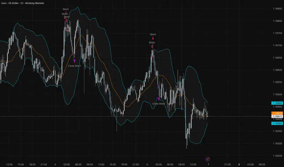
Trend Tracer [AlgoAlpha]🟠 OVERVIEW
This tool builds a two-stage trend model that reacts to structure shifts while also showing how strong or weak the move is. It uses a mid-price band (from the highest high and lowest low over a lookback) and applies two Supertrend passes on top of it. The first pass smoothens the basis. The second pass refines that direction and produces the final trail used for signals. A gradient fill between the two trails uses RSI of price-to-trail distance to show when price is stretched or cooling off. The aim is to give traders a simple way to read trend alignment, pressure, and early turns without guessing.
🟠 CONCEPTS
The script starts with a mid-range basis. This is the average of the rolling highest high and lowest low. It acts as a stable structure reference instead of raw close or typical price. From there, two Supertrend layers are applied:
• The first Supertrend uses a shorter ATR period and lower factor. It reacts faster and sets the main regime.
• The second Supertrend uses a slightly longer ATR and higher factor. It filters noise, waits for confirmed continuation, and generates the signal line.
The interaction between these trails matters. The outer Supertrend provides context by defining the broader regime. The inner Supertrend provides timing by flipping earlier and marking possible shifts. The gradient fill uses RSI of (close − supertrend value) to display when price stretches away from the trail. This shows strength, exhaustion, or compression within the trend.
🟠 FEATURES
Bullish and bearish flip markers placed at recent highs/lows
Rejection signals off the trend tracer line
Alerts for bullish and bearish trend changes
🟠 USAGE
Setup : Add the script to your chart. Timeframe is flexible; lower timeframes show more flips while higher ones give cleaner swings. Adjust Length to change how wide the basis range is. Use the two ATR settings and factors to match the volatility of the market you trade.
Read the chart : When the refined trail (stv_) sits above price the regime is bearish; when below, it is bullish. The wide trail (stv) confirms the larger move. Watch the gradient fill: darker colors appear when price is stretched from the trail and lighter colors appear when the move is weakening. Flip markers ▲ or ▼ highlight the first clean shift of the refined trail.
Settings that matter : Increasing the Main Factor slows main-trend flips and filters chop. Increasing the Signal Factor delays the timing trail but reduces noise. Shortening Length makes the basis more reactive. ATR periods change how sensitive each Supertrend pass is to volatility.