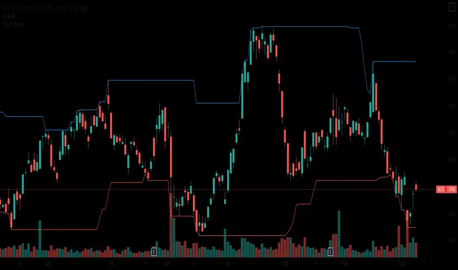
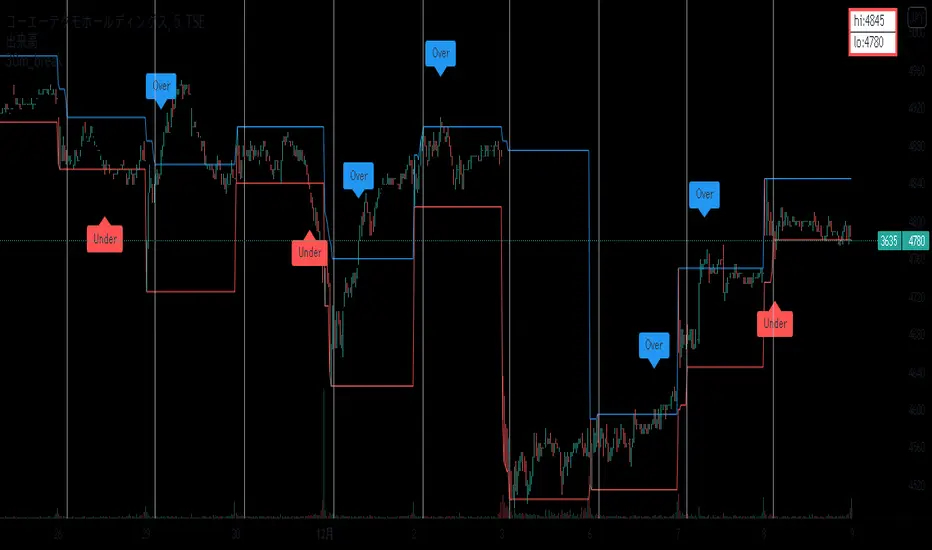
30min_breakEnglish:
It is an indicator that displays the high and low prices as of 30 minutes before the event,
and when you break it, you can see it with a balloon.
The high and low lines at 30 minutes before the front are shown as candidates for support lines and resistance lines.
Used in the minute chart
Japanese:
前場 30分時点の 高値・安値の線を表示し、そこをBreakしたら吹き出しでわかるようにしたインジケーターです
前場 30分時点の 高値安値の線を支持線・抵抗線の候補として図示します。
分足のチャートで利用します
Поиск скриптов по запросу "价格在30元内股票"
30min_breakEnglish:
It is an indicator that displays the high and low prices as of 30 minutes before the event,
and when you break it, you can see it with a balloon.
The high and low lines at 30 minutes before the front are shown as candidates for support lines and resistance lines.
Used in the minute chart
Japanese:
前場 30分時点の 高値・安値の線を表示し、そこをBreakしたら吹き出しでわかるようにしたインジケーターです
前場 30分時点の 高値安値の線を支持線・抵抗線の候補として図示します。
分足のチャートで利用します
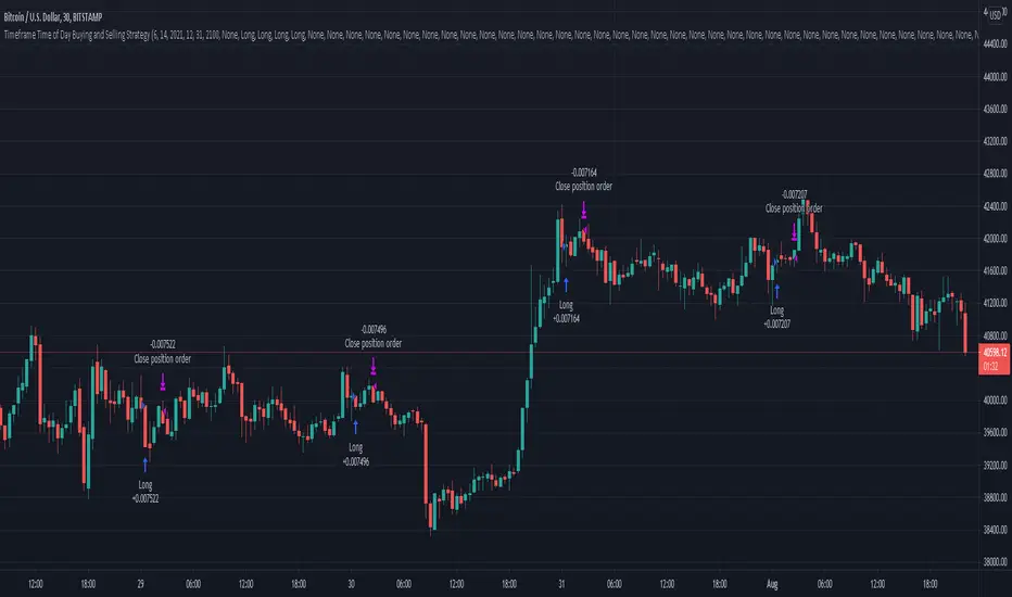
Timeframe Time of Day Buying and Selling StrategyThis strategy allows you to back test longing or shorting or do nothing during time increments of 30 minutes. The price trends in one direction every 30 minutes and this strategy allows you to test various 30 minute time frames across a range of dates to capitalize on this.
Make sure you are in the 30 minute time frame while viewing the performance and trade history.
McClellan Oscillator for DAX (GER30) [aftabmk modified]About McClellan Oscillator
Developed by Sherman and Marian McClellan, the McClellan Oscillator is a breadth indicator derived from Net Advances, the number of advancing issues less the number of declining issues. Subtracting the 39-day exponential moving average of Net Advances from the 19-day exponential moving average of Net Advances forms the oscillator.
As the formula reveals, the McClellan Oscillator is a momentum indicator that works similar to MACD .
McClellan Oscillator signals can be generated with breadth thrusts, centerline crossovers, overall levels and divergences.
About my version
This version here is a modification, though:
- It can only be used on the DAX index (DAX 30 or GER 30)
- It only considers the DAX 30 stocks
- The data window will provide a summary about rising and declining stocks
- The data window will output the last change for each of the 30 stocks
BUG
I am only publishing this version because I am not sure if my current version is saved when I leave tradingview.com without publishing the script.
This version still contains a bug - the if/else clauses do not correctly recognize declining stocks. So the oscillator should not be used as it is.
Working on it these days. Feel free to provide feedback!
Stuff I am working on
- Coloring the area green/red according to the value
- Fixing this bug/making this script more efficient
DISCLAIMER
This script was mainly written for educational purposes (training myself how to write custom indicatotors).
As you can see, the code is really messy.
Credits
Based on the simple version of aftabmk
You can find the original version by searching for McClellan Oscillator for nifty 50.

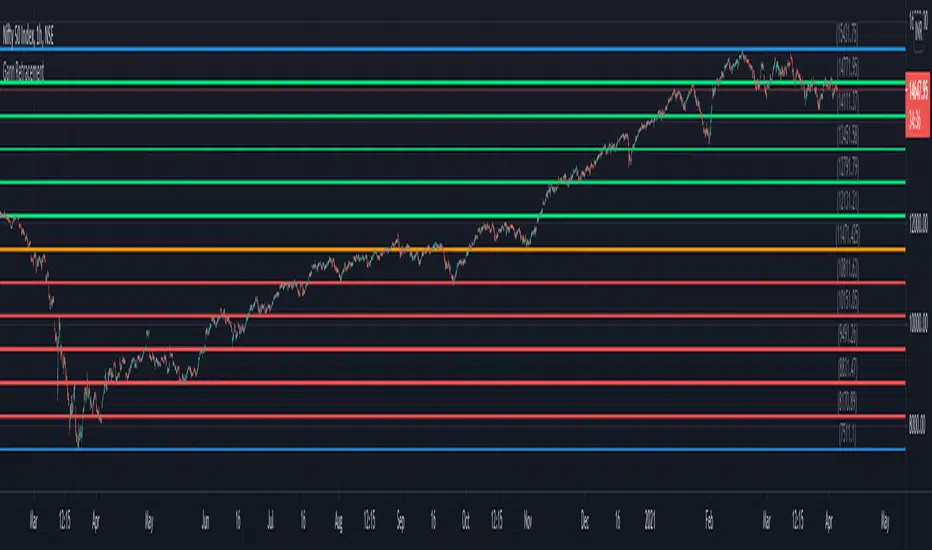
Gann RetracementThe indicator is based on W. D. Gann's method of retracement studies. Gann looked at stock retracement action in terms of Halves (1/2), Thirds (1/3, 2/3), Fifths (1/5, 2/5, 3/5, and 4/5) and more importantly the Eighths (1/8, 2/8, 3/8, 4/8, 5/8, 6/8, and 7/8). Needless to say, {2, 3, 5, 8} are the only Fibonacci numbers between 1 to 10. These ratios can easily be visualized in the form of division of a Circle as follows :
Divide the circle in 12 equal parts of 30 degree each to produce the Thirds :
30 x 4 = 120 is 1/3 of 360
30 x 8 = 240 is 2/3 of 360
The 30 degree retracement captures fundamental geometric shapes like a regular Triangle (120-240-360), a Square (90-180-270-360), and a regular Hexagon (60-120-180-240-300-360) inscribed inside of the circle.
Now, divide the circle in 10 equal parts of 36 degree each to produce the Fifths :
36 x 2 = 72 is 1/5 of 360
36 x 4 = 144 is 2/5 of 360
36 x 6 = 216 is 3/5 of 360
36 x 8 = 288 is 4/5 of 360
where, (72-144-216-288-360) is a regular Pentagon.
Finally, divide the circle in 8 equal parts of 45 degree each to produce the Eighths :
45 x 1 = 45 is 1/8 of 360
45 x 2 = 90 is 2/8 of 360
45 x 3 = 135 is 3/8 of 360
45 x 4 = 180 is 4/8 of 360
45 x 5 = 225 is 5/8 of 360
45 x 6 = 270 is 6/8 of 360
45 x 7 = 315 is 7/8 of 360
where, (45-90-135-180-225-270-315-360) is a regular Octagon.
How to Use this indicator ?
The indicator generates Gann retracement levels between any two significant price points, such as a high and a low.
Input :
Swing High (significant high price point, such as a top)
Swing Low (significant low price point, such as a bottom)
Degree (degree of retracement)
Output :
Gann retracement levels (color coded as follows) :
Swing High and Swing Low (BLUE)
50% retracement (ORANGE)
Retracements between Swing Low and 50% level (RED)
Retracements between 50% level and Swing High (LIME)
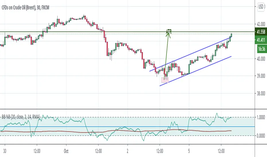
Bollinger Bands %B + ATR This indicator is best suitable for the 30-minutes interval OIL charts, due to ATR accuracy.
BB%B is great for showing oversold/overbought market conditions and offers excellent entry/exit opportunities for Day Trading (30 minutes chart), as well as reliable convergence/divergence patterns. ATR is conveniently combined and shows potential market volatility levels for the day when used in 30-minutes charts, thus demarcating your day trade exit point.
To use the ATR on this indicator: Just read the ATR value of the lowest (for a new bull trend) or the highest (for a new bear trend) candlestick of the newly formed trend leg. Let's suppose the ATR reads 0.2891, then you project a move of 2.891 points towards the given trend direction using the ruler tool (30-minutes charts). That's all, and there you have your take profit target!
Good Luck!!!
ADX strategy (considering ADX and +DI only )I have been checking the strategies on ADX indicator.
I have found that +DI crossing above ADX line under threshold 30 and exit on crossdown when ADX above 30 has better results than just following crossovers of +DI and -DI , ADX crossing above 30 .
BUY Rule
========
fast ema is above slow ema (default 13 and 55 , you can change these values in settings)
+DI cross above ADX well beloe threshold level (default 30)
Exit reule
========
when +DI cross down ADX , well above on threshold level
Stop Loss
=========
Default is set to 8%
Take a look and let me know how your symbol works with this strategy
Note : Bar color changes to yellow when the BUY condition is met.
Bar color and Background color shows to blue --- if Long position is active
fast ema and long ema doesnt print on the chart -- please add manually to the chart
Warning : for the use of educational purposes only

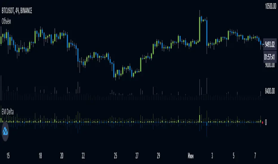
EulerMethod: DeltaEN
Shows the Integral Volume Delta (IVD)
It is a detailed OBV. Each bar sums up the volume for bars of a shorter timeframe.
For example, inside a 1M bar, every 12h bar is added up, and inside a 1h bar, every 1min bar is added. Thus, a conditional volume delta inside the bar is obtained.
The indicator for each bar shows the volume of purchases (positive), sales (negative) and the difference — IVD
The delta histogram is thicker than the volume histograms
Settings detalisation
M — 6 hours, 12 hours and 1 day for the M timeframe (720 by default)
W — 4 hours, 6 hours and 12 hours for the W timeframe (240 by default)
D — 30 minutes, 1 hour and 2 hours for the D timeframe (60 by default)
H — 1 minute, 5 minutes and 15 minutes for timeframes [1h, D) (default is 1)
For timeframes of 15m and less, the calculation is carried out by minute bars
VSA mode
The classic OBV adds volume to the cumulative sum under the condition Сlose (n) > Close (n-1) and subtracts it under the condition Close (n) < Close (n-1)
When VSA mode is disabled, all volumes are summed up under these conditions.
When the VSA approximation is turned on, the volume per bar of detail is divided by the factor (Close - Low) / (High - Low)
That is, it takes into account the spread per bar and closing relative to the spread. VSA is enabled by default
A/D mode
Shows the cumulative Accumulation / Distribution Index
The delta of the detail bar is multiplied by (High + Low + Close) / 3 bars, the result is added to the cumulative sum
No additional price conversions required due to integral summation
Index line view is customizable
EM Delta does not receive intermediate values in real time.
To see the result, wait until the bar closes or switch to a smaller timeframe
RU
Показывает Интегральную Дельту Объёма (ИДО)
Представляет собой детализированный OBV. В каждом баре суммируется объём за бары меньшего таймфрейма.
Например, внутри 1М-бара суммируется каждый 12h-бар, а внутри 1h — каждый 1m-бар. Таким образом получается условная дельта объёма внутри бара
Индикатор на каждый бар показывает объём покупок (положительный), объём продаж (отрицательный) и разницу — ИДО
Гистограмма дельты толще гистограмм объёмов
Настройки детализации внутри бара
M — 6 часов, 12 часов и 1 день для таймфрейма M (по-умолчанию 720)
W — 4 часа, 6 часов и 12 часов для таймфрейма W (по-умолчанию 240)
D — 30 минут, 1 час и 2 часа для таймфрейма D (по-умолчанию 60)
H — 1 минута, 5 минут и 15 минут для таймфреймов [1h, D) (по-умолчанию 1)
Для таймфреймов 15m и меньше расчёт ведётся по минутным барам
Режим VSA
Классический OBV прибавляет объём к кумулятивной сумме при условии Сlose(n) > Close(n-1) и отнимает при условии Close(n) < Close(n-1)
При отключении режима VSA все объёмы суммируются по этим условиям
При включённой VSA-аппроксимации объём за бар детализации делится по фактору (Close - Low) / (High - Low)
То есть учитывает спред за бар и закрытие относительно спреда. По-умолчанию режим VSA включен
Режим A/D
Показывает кумулятивный индекс Накопления/Распределения
Дельта бара детализации умножается на (High + Low + Close) / 3 бара, результат прибавляется к кумулятивной сумме
Дополнительные преобразования цены не требуются ввиду интегрального суммирования
Вид линии индекса настраивается
EM Delta не получает промежуточные значения в реальном времени.
Чтобы увидеть результат, дождитесь закрытия бара или перейдите на меньший таймфрейм
Crypto Trading Hours UTC based on Berlin time (UTC +2)Although crypto markets trade 24/7, there are spikes in volume according to the general hours at which different parts of the world do the majority of their trading.
This Script highlights the US, European and Asian markets when they are most active. The normal market hours are always from 08:00 to 16:30 local time.
US market opens at 8:00 Silicon Valley local time, and closes at 16:30 New York local time.
European market opens at 8:00 London local time, and closes at 16:30 Frankfurt local time.
Asian market opens at 8:00 Hong Kong local time, and closes at 16:30 Sydney local time.

Supertrend MTF LAG ISSUEThis script based on
we all use Super trend but it main issue is the lag as it buy too late or sell too late
using Deavaet study of Heat map MTF we can do a little trick
if you look on his study you can see that major signal for example will happen in the time frame before it happen at larger time frame
so in this example if signal at MTF 30 min and signal at MTF 60 min happen at the same time at 2 hours or 4 hours candles then this signal are more likely to be true then random signal at each time frame specific.
since we use shorter time frame on larger time frame we can remove the lag issue that make supertrend not so effective
In this example I set the signal to be MTF 30 +60 om 2 hour TF , can be good also for 4 hour candles..
So you get the signal to close inside the larger candle
now if you want to make on even shorter TF then change the code to 15 and 30 MTF on candles on 1 hour
or 1 and 5 min on 30 min or 15 min

Panchang Time//This indicator is required in NimblrTA and can be used to define timeslots for the trend confirmation
study("Panchang Time", overlay=true)
timeinrange(res, sess) => time(res, sess) != 0
premarket = #C0C0C0
regular = #0000FF
regularslot2 = #00CCFF
postmarket = #5000FF
notrading = na
sessioncolor = timeinrange("30", "0915-0930") ? premarket : timeinrange("30", "0915-0930") ? regular : timeinrange("30", "0931-1200") ? regularslot2 : timeinrange("30", "1201-1305") ? postmarket : notrading
bgcolor(sessioncolor, transp=90)

extended session - Regular Opening-Range- JayyOpening Range and some other scripts updated to plot correctly (see comments below.) There are three variations of the fibonacci expansion beyond the opening range and retracements within the opening range of the US Market session - I have not put in the script for the other markets yet.
The three scripts have different uses and strengths:
The extended session script (with the script here below) will plot the opening range whether you are using the extended session or the regular session. (that is to say whether "ext" in the lower right hand corner is highlighted or not.). While in the extended session the opening range has some plotting issues with periods like 13 minutes or any period that is not divisible into 330 mins with a round number outcome (eg 330/60 =5.5. Therefore an hour long opening range has problems in the extended session.
The pre session script is only for the premarket. You can select any opening range period you like. I have set the opening range to be the full premarket session. If you select a different session you will have to unselect "pre open to 9:30 EST for Opening Range?" in the format section. The script defaults to 15 minutes in the "period Of Pre Opening Range?". To go back to the 4 am to 9:30 pre opening range select "pre open to 9:30 EST for Opening Range?" there is no automatic 330 minute selection.
The past days offset script only works in 5 min or 15 minute period. It will show the opening range from up to 20 days past over the current days price action. Use this for the regular session only. 0 shows the current day's opening range. Use the positive integers for number of days back ie 1, 2, 3 etc not -1, -2, -3 etc. The script is preprogrammed to use the current day (0).
Scripts updated to plot correctly: One thing they all have in common is a way of they deal with a somewhat random problem that shifts the plots 4 hours in one direction or the other ie the plot started at 9:30 EST or 1:30PM EST. This issue started to occur approximately June 22, 2015 and impacts any script that tried to use "session" times to manage a plot in my scripts. The issue now seems to have been resolved during this past week.
Just in case the problem reoccurs I have added a "Switch session plot?" to each script. If the plot looks funny check or uncheck the "Switch session plot?" and see the difference. Of course if a new issue crops up it will likely require a different fix.
I have updated all of the scripts shown on this chart. If you are using a script of mine that suffers from the compiler issue then you will find an update on this chart. You can get any and all of the scripts by clicking on the small sideways wishbone on the left middle of the chart. You will see a dialogue box. Then click "make it mine". This will import all of the scripts to your computer and you can play around with them all to decide what you want and what you don't want. This is the easiest way to get all of the scripts in one fell swoop. It is also the easiest way for me to make all of the scripts available. I do not have all of the plots visible since it is too messy and one of the scripts (pre OR) is only for the regular session. To view the scripts click on the blue eye to the right of the script title to show it on this script. If you can only use the regular session. The scripts will all (with the exception of the pre OR) work fine.
If for any reason this script seems flakey refresh the page r try a slightly different period. I have noticed that sometimes randomly the script loves to return to the 5 min OR. This is a very new issue transient issue. As always if you see an issue please let me know.
Cheers Jayy
Moving VWAP-KAMA CloudMoving VWAP-KAMA Cloud
Overview
The Moving VWAP-KAMA Cloud is a high-conviction trend filter designed to solve a major problem with standard indicators: Noise. By combining a smoothed Volume Weighted Average Price (MVWAP) with Kaufman’s Adaptive Moving Average (KAMA), this indicator creates a "Value Zone" that identifies the true structural trend while ignoring choppy price action.
Unlike brittle lines that break constantly, this cloud is "slow" by design—making it exceptionally powerful for spotting genuine trend reversals and filtering out fakeouts.
How It Works
This script uses a unique "Double Smoothing" architecture:
The Anchor (MVWAP): We take the standard VWAP and smooth it with a 30-period EMA. This represents the "Fair Value" baseline where volume has supported price over time.
The Filter (KAMA): We apply Kaufman's Adaptive Moving Average to the already smoothed MVWAP. KAMA is unique because it flattens out during low-volatility (choppy) periods and speeds up during high-momentum trends.
The Cloud:
Green/Teal Cloud: Bullish Structure (MVWAP > KAMA)
Purple Cloud: Bearish Structure (MVWAP < KAMA)
🔥 The "Reversal Slingshot" Strategy
Backtests reveal a powerful behavior during major trend changes, particularly after long bear markets:
The Resistance Phase: During a long-term downtrend, price will repeatedly rally into the Purple Cloud and get rejected. The flattened KAMA line acts as a "concrete ceiling," keeping the bearish trend intact.
The Breakout & Flip: When price finally breaks above the cloud with conviction, and the cloud flips Green, it signals a structural regime change.
The "Slingshot" Retest: Often, immediately after this flip, price will drop back into the top of the cloud. This is the "Slingshot" moment. The old resistance becomes new, hardened support.
The Rally: From this support bounce, stocks often launch into a sustained, multi-month bull run. This setup has been observed repeatedly at the bottom of major corrections.
How to Use This Indicator
1. Dynamic Support & Resistance
The KAMA Wall: When price retraces into the cloud, the KAMA line often flattens out, acting as a hard "floor" or "wall." A break of this wall usually signals a genuine trend change, not just a stop hunt.
2. Trend Confirmation (Regime Filter)
Bullish Regime: If price is holding above the cloud, only look for Long setups.
Bearish Regime: If price is holding below the cloud, only look for Short setups.
No-Trade Zone: If price is stuck inside the cloud, the market is traversing fair value. Stand aside until a clear winner emerges.
3. Multi-Timeframe Versatility
While designed for trend confirmation on higher timeframes (4H, Daily), this indicator adapts beautifully to lower timeframes (5m, 15m) for intraday scalping.
On Lower Timeframes: The cloud reacts much faster, acting as a dynamic "VWAP Band" that helps intraday traders stay on the right side of momentum during the session.
Settings
Moving VWAP Period (30): The lookback period for the base VWAP smoothing.
KAMA Settings (10, 10, 30): Controls the sensitivity of the adaptive filter.
Cloud Transparency: Adjust to keep your chart clean.
Alerts Included
Price Cross Over/Under MVWAP
Price Cross Over/Under KAMA
Cloud Flip (Bullish/Bearish Trend Change)
Tip for Traders
This is not a signal entry indicator. It is a Trend Conviction tool. Use it to filter your entries from faster indicators (like RSI or MACD). If your fast indicator signals "Buy" but the cloud is Purple, the probability is low. Wait for the Cloud Flip

Smart RSI MTF Matrix [DotGain]Summary
Are you tired of trading trend signals, only to miss the bigger picture because you are focused on a single timeframe?
The Smart RSI MTF Matrix is the ultimate "Cockpit View" for momentum traders. Unlike chart overlays that can sometimes clutter your price action, this indicator organizes RSI conditions across 10 different timeframes simultaneously into a clean, separate Heatmap pane.
It monitors everything from the 5-minute chart all the way up to the 12-Month view , giving you a complete X-ray vision of the market's momentum structure instantly.
⚙️ Core Components and Logic
The Smart RSI MTF Matrix relies on a sophisticated hierarchy to deliver clear, actionable context:
Multi-Timeframe Engine: The script runs 10 independent RSI calculations in the background, organized in rows from bottom (Short Term) to top (Long Term).
Classic RSI Thresholds:
Overbought (> 70): Indicates price may be extended to the upside.
Oversold (< 30): Indicates price may be extended to the downside.
Smart Visibility System (The "Secret Sauce"): Not all signals are equal. A 5-minute signal is "noise" compared to a Yearly signal. This indicator automatically applies Transparency to differentiate importance. The visibility increases by 10% for each higher timeframe slot (Row).
🚦 How to Read the Matrix
The indicator plots dots in 10 stacked rows. The position and opacity tell you the direction and significance:
🟥 RED DOTS (Overbought Condition)
Trigger: RSI is above 70 on that specific timeframe.
Meaning: Potential bearish reversal or pullback.
🟩 GREEN DOTS (Oversold Condition)
Trigger: RSI is below 30 on that specific timeframe.
Meaning: Potential bullish reversal or bounce.
⚪ GRAY DOTS (Neutral)
Trigger: RSI is between 30 and 70.
Meaning: No extreme momentum present.
👻 TRANSPARENCY (Signal Strength)
The visibility of the dot tells you exactly which Timeframe (Row) is triggered. The higher the row, the more solid the color:
Faint (10-30% Visibility): Rows 1-3 (5m, 15m, 1h). Used for scalping entries.
Medium (40-60% Visibility): Rows 4-6 (4h, 1D, 1W). Used for swing trading context.
Solid (70-100% Visibility): Rows 7-10 (1M, 3M, 6M, 12M). Used for identifying major macro cycles.
Visual Elements
Structure: Row 1 (Bottom) represents the 5-minute timeframe. Row 10 (Top) represents the 12-Month timeframe.
Vertical Alignment: If you see a vertical column of Red or Green dots, it indicates Multi-Timeframe Confluence —a highly probable reversal point.
Key Benefit
The goal of the Smart RSI MTF Matrix is to keep your main chart clean while providing maximum information. You can instantly see if a short-term pullback (Faint Green Dot) is happening within a long-term uptrend (Solid Gray/Red Dot), allowing for precision entries.
Have fun :)
Disclaimer
This "Smart RSI MTF Matrix" indicator is provided for informational and educational purposes only. It does not, and should not be construed as, financial, investment, or trading advice.
The signals generated by this tool (both "Buy" and "Sell" indications) are the result of a specific set of algorithmic conditions. They are not a direct recommendation to buy or sell any asset. All trading and investing in financial markets involves substantial risk of loss. You can lose all of your invested capital.
Past performance is not indicative of future results. The signals generated may produce false or losing trades. The creator (© DotGain) assumes no liability for any financial losses or damages you may incur as a result of using this indicator.
You are solely responsible for your own trading and investment decisions. Always conduct your own research (DYOR) and consider your personal risk tolerance before making any trades.

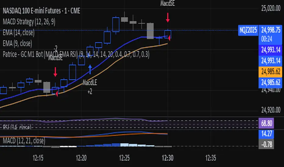
Patrice - GC M1 Bot (MACD EMA RSI)//@version=6
indicator("Patrice - GC M1 Bot (MACD EMA RSI)", overlay = true)
//----------------------
// Inputs (optimisés GC)
//----------------------
emaLenFast = input.int(9, "EMA rapide")
emaLenSlow = input.int(14, "EMA lente")
rsiLen = input.int(14, "RSI length")
atrLen = input.int(14, "ATR length")
volLen = input.int(20, "Volume moyenne")
slMult = input.float(0.4, "SL = ATR x", step = 0.1)
tpMult = input.float(0.7, "TP = ATR x", step = 0.1)
minAtr = input.float(0.7, "ATR minimum pour trader", step = 0.1)
maxDistEmaPct = input.float(0.3, "Distance max EMA9 (%)", step = 0.1)
//----------------------
// Indicateurs
//----------------------
ema9 = ta.ema(close, emaLenFast)
ema14 = ta.ema(close, emaLenSlow)
= ta.macd(close, 12, 26, 9)
hist = macdLine - signalLine
rsi = ta.rsi(close, rsiLen)
atr = ta.atr(atrLen)
volMa = ta.sma(volume, volLen)
//----------------------
// Session 9:30 - 11:00 (NY)
//----------------------
hourSession = hour(time, "America/New_York")
minuteSession = minute(time, "America/New_York")
inSession = (hourSession == 9 and minuteSession >= 30) or
(hourSession > 9 and hourSession < 11) or
(hourSession == 11 and minuteSession == 0)
//----------------------
// Filtres vol / ATR / distance EMA
//----------------------
volFilter = volume > volMa
atrFilter = atr > minAtr
distEmaPct = math.abs(close - ema9) / close * 100.0
distFilter = distEmaPct < maxDistEmaPct
//----------------------
// Tendance
//----------------------
bullTrend = close > ema9 and close > ema14 and ema9 > ema14
bearTrend = close < ema9 and close < ema14 and ema9 < ema14
//----------------------
// MACD : 2e barre
//----------------------
bullSecondBar = hist > 0 and hist > 0 and hist <= 0
bearSecondBar = hist < 0 and hist < 0 and hist >= 0
//----------------------
// Filtres RSI
//----------------------
rsiLongOk = rsi < 70 and rsi >= 45 and rsi <= 65
rsiShortOk = rsi > 30 and rsi >= 35 and rsi <= 55
//----------------------
// Gestion du risque (simple pour l'instant)
//----------------------
canTradeRisk = true
//----------------------
// Conditions d'entrée
//----------------------
longCond = bullTrend and bullSecondBar and rsiLongOk and inSession and volFilter and atrFilter and distFilter and canTradeRisk
shortCond = bearTrend and bearSecondBar and rsiShortOk and inSession and volFilter and atrFilter and distFilter and canTradeRisk
//----------------------
// SL / TP (info seulement, pas d'ordres)
//----------------------
slPoints = atr * slMult
tpPoints = atr * tpMult
longSL = close - slPoints
longTP = close + tpPoints
shortSL = close + slPoints
shortTP = close - tpPoints
//----------------------
// Visuels
//----------------------
plot(ema9, title = "EMA 9")
plot(ema14, title = "EMA 14")
plotshape(longCond, title = "Signal Long", style = shape.triangleup, location = location.belowbar, size = size.tiny, text = "L")
plotshape(shortCond, title = "Signal Short", style = shape.triangledown, location = location.abovebar, size = size.tiny, text = "S")
//----------------------
// Conditions d'ALERTE
//----------------------
alertcondition(longCond, title = "ALERTE LONG", message = "Signal LONG Patrice GC bot")
alertcondition(shortCond, title = "ALERTE SHORT", message = "Signal SHORT Patrice GC bot")
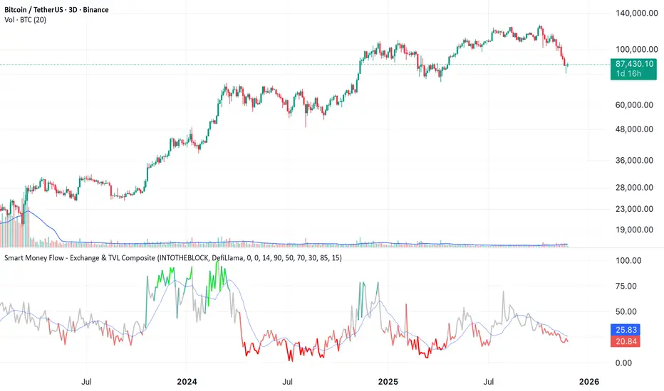
Smart Money Flow - Exchange & TVL Composite# Smart Money Flow - Exchange & TVL Composite Indicator
## Overview
The **Smart Money Flow (SMF)** indicator combines two powerful on-chain metrics - **Exchange Flows** and **Total Value Locked (TVL)** - to create a composite index that tracks institutional and "smart money" movement in the cryptocurrency market. This indicator helps traders identify accumulation and distribution phases by analyzing where capital is flowing.
## What It Does
This indicator normalizes and combines:
- **Exchange Net Flow** (from IntoTheBlock): Tracks Bitcoin/Ethereum movement to and from exchanges
- **Total Value Locked** (from DefiLlama): Measures capital locked in DeFi protocols
The composite index is displayed on a 0-100 scale with clear zones for overbought/oversold conditions.
## Core Concept
### Exchange Flows
- **Negative Flow (Outflows)** = Bullish Signal
- Coins moving OFF exchanges → Long-term holding/accumulation
- Indicates reduced selling pressure
- **Positive Flow (Inflows)** = Bearish Signal
- Coins moving TO exchanges → Preparation for selling
- Indicates potential distribution phase
### Total Value Locked (TVL)
- **Rising TVL** = Bullish Signal
- Capital flowing into DeFi protocols
- Increased ecosystem confidence
- **Falling TVL** = Bearish Signal
- Capital exiting DeFi protocols
- Decreased ecosystem confidence
### Combined Signals
**🟢 Strong Bullish (70-100):**
- Exchange outflows + Rising TVL
- Smart money accumulating and deploying capital
**🔴 Strong Bearish (0-30):**
- Exchange inflows + Falling TVL
- Smart money preparing to sell and exiting positions
**⚪ Neutral (40-60):**
- Mixed or balanced flows
## Key Features
### ✅ Auto-Detection
- Automatically detects chart symbol (BTC/ETH)
- Uses appropriate exchange flow data for each asset
### ✅ Weighted Composite
- Customizable weights for Exchange Flow and TVL components
- Default: 50/50 balance
### ✅ Normalized Scale
- 0-100 index scale
- Configurable lookback period for normalization (default: 90 days)
### ✅ Signal Zones
- **Overbought**: 70+ (Strong bullish pressure)
- **Oversold**: 30- (Strong bearish pressure)
- **Extreme**: 85+ / 15- (Very strong signals)
### ✅ Clean Interface
- Minimal visual clutter by default
- Only main index line and MA visible
- Optional elements can be enabled:
- Background color zones
- Divergence signals
- Trend change markers
- Info table with detailed metrics
### ✅ Divergence Detection
- Identifies when price diverges from smart money flows
- Potential reversal warning signals
### ✅ Alerts
- Extreme overbought/oversold conditions
- Trend changes (crossing 50 line)
- Bullish/bearish divergences
## How to Use
### 1. Trend Confirmation
- Index above 50 = Bullish trend
- Index below 50 = Bearish trend
- Use with price action for confirmation
### 2. Reversal Signals
- **Extreme readings** (>85 or <15) suggest potential reversal
- Look for divergences between price and indicator
### 3. Accumulation/Distribution
- **70+**: Accumulation phase - smart money buying/holding
- **30-**: Distribution phase - smart money selling
### 4. DeFi Health
- Monitor TVL component for DeFi ecosystem strength
- Combine with exchange flows for complete picture
## Settings
### Data Sources
- **Exchange Flow**: IntoTheBlock real-time data
- **TVL**: DefiLlama aggregated DeFi TVL
- **Manual Mode**: For testing or custom data
### Indicator Settings
- **Smoothing Period (MA)**: Default 14 periods
- **Normalization Lookback**: Default 90 days
- **Exchange Flow Weight**: Adjustable 0-100%
- **Overbought/Oversold Levels**: Customizable thresholds
### Visual Options
- Show/Hide Moving Average
- Show/Hide Zone Lines
- Show/Hide Background Colors
- Show/Hide Divergence Signals
- Show/Hide Trend Markers
- Show/Hide Info Table
## Data Requirements
⚠️ **Important Notes:**
- Uses **daily data** from IntoTheBlock and DefiLlama
- Works on any chart timeframe (data updates daily)
- Auto-switches between BTC and ETH based on chart
- All other crypto charts default to BTC exchange flow data
## Best Practices
1. **Use on Daily+ Timeframes**
- On-chain data is daily, most effective on D/W/M charts
2. **Combine with Price Action**
- Use as confirmation, not standalone signals
3. **Watch for Divergences**
- Price making new highs while indicator falling = warning
4. **Monitor Extreme Zones**
- Sustained readings >85 or <15 indicate strong conviction
5. **Context Matters**
- Consider broader market conditions and fundamentals
## Calculation
1. **Exchange Net Flow** = Inflows - Outflows (inverted for index)
2. **TVL Rate of Change** = % change over smoothing period
3. **Normalize** both metrics to 0-100 scale
4. **Composite Index** = (ExchangeFlow × Weight) + (TVL × Weight)
5. **Smooth** with moving average
## Disclaimer
This indicator uses on-chain data for analysis. While valuable, it should not be used as the sole basis for trading decisions. Always combine with other technical analysis tools, fundamental analysis, and proper risk management.
On-chain data reflects blockchain activity but may lag price action. Use this indicator as part of a comprehensive trading strategy.
---
## Credits
**Data Sources:**
- IntoTheBlock: Exchange flow metrics
- DefiLlama: Total Value Locked data
**Indicator by:** @iCD_creator
**Version:** 1.0
**Pine Script™ Version:** 6
---
## Updates & Support
For questions, suggestions, or bug reports, please comment below or message the author.
**Like this indicator? Leave a 👍 and share your feedback!**
Hash Supertrend [Hash Capital Research]Hash Supertrend Strategy by Hash Capital Research
Overview
Hash Supertrend is a professional-grade trend-following strategy that combines the proven Supertrend indicator with institutional visual design and flexible time filtering.
The strategy uses ATR-based volatility bands to identify trend direction and executes position reversals when the trend flips.This implementation features a distinctive fluorescent color system with customizable glow effects, making trend changes immediately visible while maintaining the clean, professional aesthetic expected in quantitative trading environments.
Entry Signals:
Long Entry: Price crosses above the Supertrend line (trend flips bullish)
Short Entry: Price crosses below the Supertrend line (trend flips bearish)
Controls the lookback period for volatility calculation
Lower values (7-10): More sensitive to price changes, generates more signals
Higher values (12-14): Smoother response, fewer signals but potentially delayed entries
Recommended range: 7-14 depending on market volatility
Factor (Default: 3.0)
Restricts trading to specific hours
Useful for avoiding low-liquidity sessions, overnight gaps, or known choppy periods
When disabled, strategy trades 24/7
Start Hour (Default: 9) & Start Minute (Default: 30)
Define when the trading session begins
Uses exchange timezone in 24-hour format
Example: 9:30 = 9:30 AM
End Hour (Default: 16) & End Minute (Default: 0)
Controls the vibrancy of the fluorescent color system
1-3: Subtle, muted colors
4-6: Balanced, moderate saturation
7-10: Bright, highly saturated fluorescent appearance
Affects both the Supertrend line and trend zones
Glow Effect (Default: On)
Adds luminous halo around the Supertrend line
Creates a multi-layered visual with depth
Particularly effective during strong trends
Glow Intensity (Default: 5.0)
Displays tiny fluorescent dots at entry points
Green dot below bar: Long entry
Red dot above bar: Short entry
Provides clear visual confirmation of executed trades
Show Trend Zone (Default: On)
Strong trending markets (2020-style bull runs, sustained bear markets)
Markets with clear directional bias
Instruments with consistent volatility patterns
Timeframes: 15m to Daily (optimal on 1H-4H)
Challenging Conditions:
Choppy, range-bound markets
Low volatility consolidation periods
Highly news-driven instruments with frequent gaps
Very low timeframes (1m-5m) prone to noise
Recommended AssetsCryptocurrency:

Steff- OBX- DTA OBX – US Open 15-Minute Zone Indicator
This indicator highlights the first 15 minutes of the U.S. stock market opening, also known as the OBX (Opening Balance Extension).
It is designed specifically for Nasdaq and S&P 500, which open at 09:30 New York time — corresponding to 15:30 Danish time.
What this indicator does:
• Marks the price range from 09:30–09:45 (U.S. time) as a zone on your chart
• Automatically adjusts to your local timezone, so the zone always aligns with Danish time
• Extends the zone to the right so you can track how price interacts with OBX throughout the day
• Draws all historical OBX zones so you can analyze previous reactions
• Rebuilds zones automatically when switching timeframes
• Detects breakouts from the zone
• Tracks balancing time only after a real breakout occurs
• Can automatically remove a zone if price spends a continuous amount of time inside it after the breakout (you set the minutes yourself)
• Allows full customization of OBX start time, duration, and behavior
• Individual zones can be manually deleted without being redrawn by the indicator
Why the OBX matters:
The OBX represents one of the most influential time windows in intraday trading because it reflects:
• The first injection of liquidity after the U.S. market opens
• Institutional positioning and algorithmic adjustments
• Early volatility and directional bias
• Common zones for reversals, breakouts, or mean reversion
• Key high-probability reaction levels used by professional traders
This indicator gives you a clear visual representation of when the market reacts to the U.S. open and how price interacts with the opening range throughout the session.

Kripto Fema ind/ This Pine Script™ code is subject to the terms of the Mozilla Public License 2.0 at mozilla.org
// © Femayakup
//@version=5
indicator(title = "Kripto Fema ind", shorttitle="Kripto Fema ind", overlay=true, format=format.price, precision=2,max_lines_count = 500, max_labels_count = 500, max_bars_back=500)
showEma200 = input(true, title="EMA 200")
showPmax = input(true, title="Pmax")
showLinreg = input(true, title="Linreg")
showMavilim = input(true, title="Mavilim")
showNadaray = input(true, title="Nadaraya Watson")
ma(source, length, type) =>
switch type
"SMA" => ta.sma(source, length)
"EMA" => ta.ema(source, length)
"SMMA (RMA)" => ta.rma(source, length)
"WMA" => ta.wma(source, length)
"VWMA" => ta.vwma(source, length)
//Ema200
timeFrame = input.timeframe(defval = '240',title= 'EMA200 TimeFrame',group = 'EMA200 Settings')
len200 = input.int(200, minval=1, title="Length",group = 'EMA200 Settings')
src200 = input(close, title="Source",group = 'EMA200 Settings')
offset200 = input.int(title="Offset", defval=0, minval=-500, maxval=500,group = 'EMA200 Settings')
out200 = ta.ema(src200, len200)
higherTimeFrame = request.security(syminfo.tickerid,timeFrame,out200 ,barmerge.gaps_on,barmerge.lookahead_on)
ema200Plot = showEma200 ? higherTimeFrame : na
plot(ema200Plot, title="EMA200", offset=offset200)
//Linreq
group1 = "Linreg Settings"
lengthInput = input.int(100, title="Length", minval = 1, maxval = 5000,group = group1)
sourceInput = input.source(close, title="Source")
useUpperDevInput = input.bool(true, title="Upper Deviation", inline = "Upper Deviation", group = group1)
upperMultInput = input.float(2.0, title="", inline = "Upper Deviation", group = group1)
useLowerDevInput = input.bool(true, title="Lower Deviation", inline = "Lower Deviation", group = group1)
lowerMultInput = input.float(2.0, title="", inline = "Lower Deviation", group = group1)
group2 = "Linreg Display Settings"
showPearsonInput = input.bool(true, "Show Pearson's R", group = group2)
extendLeftInput = input.bool(false, "Extend Lines Left", group = group2)
extendRightInput = input.bool(true, "Extend Lines Right", group = group2)
extendStyle = switch
extendLeftInput and extendRightInput => extend.both
extendLeftInput => extend.left
extendRightInput => extend.right
=> extend.none
group3 = "Linreg Color Settings"
colorUpper = input.color(color.new(color.blue, 85), "Linreg Renk", inline = group3, group = group3)
colorLower = input.color(color.new(color.red, 85), "", inline = group3, group = group3)
calcSlope(source, length) =>
max_bars_back(source, 5000)
if not barstate.islast or length <= 1
else
sumX = 0.0
sumY = 0.0
sumXSqr = 0.0
sumXY = 0.0
for i = 0 to length - 1 by 1
val = source
per = i + 1.0
sumX += per
sumY += val
sumXSqr += per * per
sumXY += val * per
slope = (length * sumXY - sumX * sumY) / (length * sumXSqr - sumX * sumX)
average = sumY / length
intercept = average - slope * sumX / length + slope
= calcSlope(sourceInput, lengthInput)
startPrice = i + s * (lengthInput - 1)
endPrice = i
var line baseLine = na
if na(baseLine) and not na(startPrice) and showLinreg
baseLine := line.new(bar_index - lengthInput + 1, startPrice, bar_index, endPrice, width=1, extend=extendStyle, color=color.new(colorLower, 0))
else
line.set_xy1(baseLine, bar_index - lengthInput + 1, startPrice)
line.set_xy2(baseLine, bar_index, endPrice)
na
calcDev(source, length, slope, average, intercept) =>
upDev = 0.0
dnDev = 0.0
stdDevAcc = 0.0
dsxx = 0.0
dsyy = 0.0
dsxy = 0.0
periods = length - 1
daY = intercept + slope * periods / 2
val = intercept
for j = 0 to periods by 1
price = high - val
if price > upDev
upDev := price
price := val - low
if price > dnDev
dnDev := price
price := source
dxt = price - average
dyt = val - daY
price -= val
stdDevAcc += price * price
dsxx += dxt * dxt
dsyy += dyt * dyt
dsxy += dxt * dyt
val += slope
stdDev = math.sqrt(stdDevAcc / (periods == 0 ? 1 : periods))
pearsonR = dsxx == 0 or dsyy == 0 ? 0 : dsxy / math.sqrt(dsxx * dsyy)
= calcDev(sourceInput, lengthInput, s, a, i)
upperStartPrice = startPrice + (useUpperDevInput ? upperMultInput * stdDev : upDev)
upperEndPrice = endPrice + (useUpperDevInput ? upperMultInput * stdDev : upDev)
var line upper = na
lowerStartPrice = startPrice + (useLowerDevInput ? -lowerMultInput * stdDev : -dnDev)
lowerEndPrice = endPrice + (useLowerDevInput ? -lowerMultInput * stdDev : -dnDev)
var line lower = na
if na(upper) and not na(upperStartPrice) and showLinreg
upper := line.new(bar_index - lengthInput + 1, upperStartPrice, bar_index, upperEndPrice, width=1, extend=extendStyle, color=color.new(colorUpper, 0))
else
line.set_xy1(upper, bar_index - lengthInput + 1, upperStartPrice)
line.set_xy2(upper, bar_index, upperEndPrice)
na
if na(lower) and not na(lowerStartPrice) and showLinreg
lower := line.new(bar_index - lengthInput + 1, lowerStartPrice, bar_index, lowerEndPrice, width=1, extend=extendStyle, color=color.new(colorUpper, 0))
else
line.set_xy1(lower, bar_index - lengthInput + 1, lowerStartPrice)
line.set_xy2(lower, bar_index, lowerEndPrice)
na
showLinregPlotUpper = showLinreg ? upper : na
showLinregPlotLower = showLinreg ? lower : na
showLinregPlotBaseLine = showLinreg ? baseLine : na
linefill.new(showLinregPlotUpper, showLinregPlotBaseLine, color = colorUpper)
linefill.new(showLinregPlotBaseLine, showLinregPlotLower, color = colorLower)
// Pearson's R
var label r = na
label.delete(r )
if showPearsonInput and not na(pearsonR) and showLinreg
r := label.new(bar_index - lengthInput + 1, lowerStartPrice, str.tostring(pearsonR, "#.################"), color = color.new(color.white, 100), textcolor=color.new(colorUpper, 0), size=size.normal, style=label.style_label_up)
//Mavilim
group4 = "Mavilim Settings"
mavilimold = input(false, title="Show Previous Version of MavilimW?",group=group4)
fmal=input(3,"First Moving Average length",group = group4)
smal=input(5,"Second Moving Average length",group = group4)
tmal=fmal+smal
Fmal=smal+tmal
Ftmal=tmal+Fmal
Smal=Fmal+Ftmal
M1= ta.wma(close, fmal)
M2= ta.wma(M1, smal)
M3= ta.wma(M2, tmal)
M4= ta.wma(M3, Fmal)
M5= ta.wma(M4, Ftmal)
MAVW= ta.wma(M5, Smal)
col1= MAVW>MAVW
col3= MAVWpmaxsrc ? pmaxsrc-pmaxsrc : 0
vdd1=pmaxsrc
ma = 0.0
if mav == "SMA"
ma := ta.sma(pmaxsrc, length)
ma
if mav == "EMA"
ma := ta.ema(pmaxsrc, length)
ma
if mav == "WMA"
ma := ta.wma(pmaxsrc, length)
ma
if mav == "TMA"
ma := ta.sma(ta.sma(pmaxsrc, math.ceil(length / 2)), math.floor(length / 2) + 1)
ma
if mav == "VAR"
ma := VAR
ma
if mav == "WWMA"
ma := WWMA
ma
if mav == "ZLEMA"
ma := ZLEMA
ma
if mav == "TSF"
ma := TSF
ma
ma
MAvg=getMA(pmaxsrc, length)
longStop = Normalize ? MAvg - Multiplier*atr/close : MAvg - Multiplier*atr
longStopPrev = nz(longStop , longStop)
longStop := MAvg > longStopPrev ? math.max(longStop, longStopPrev) : longStop
shortStop = Normalize ? MAvg + Multiplier*atr/close : MAvg + Multiplier*atr
shortStopPrev = nz(shortStop , shortStop)
shortStop := MAvg < shortStopPrev ? math.min(shortStop, shortStopPrev) : shortStop
dir = 1
dir := nz(dir , dir)
dir := dir == -1 and MAvg > shortStopPrev ? 1 : dir == 1 and MAvg < longStopPrev ? -1 : dir
PMax = dir==1 ? longStop: shortStop
plot(showsupport ? MAvg : na, color=#fbff04, linewidth=2, title="EMA9")
pALL=plot(PMax, color=color.new(color.red, transp = 0), linewidth=2, title="PMax")
alertcondition(ta.cross(MAvg, PMax), title="Cross Alert", message="PMax - Moving Avg Crossing!")
alertcondition(ta.crossover(MAvg, PMax), title="Crossover Alarm", message="Moving Avg BUY SIGNAL!")
alertcondition(ta.crossunder(MAvg, PMax), title="Crossunder Alarm", message="Moving Avg SELL SIGNAL!")
alertcondition(ta.cross(pmaxsrc, PMax), title="Price Cross Alert", message="PMax - Price Crossing!")
alertcondition(ta.crossover(pmaxsrc, PMax), title="Price Crossover Alarm", message="PRICE OVER PMax - BUY SIGNAL!")
alertcondition(ta.crossunder(pmaxsrc, PMax), title="Price Crossunder Alarm", message="PRICE UNDER PMax - SELL SIGNAL!")
buySignalk = ta.crossover(MAvg, PMax)
plotshape(buySignalk and showsignalsk ? PMax*0.995 : na, title="Buy", text="Buy", location=location.absolute, style=shape.labelup, size=size.tiny, color=color.new(color.green, transp = 0), textcolor=color.white)
sellSignallk = ta.crossunder(MAvg, PMax)
plotshape(sellSignallk and showsignalsk ? PMax*1.005 : na, title="Sell", text="Sell", location=location.absolute, style=shape.labeldown, size=size.tiny, color=color.new(color.red, transp = 0), textcolor=color.white)
// buySignalc = ta.crossover(pmaxsrc, PMax)
// plotshape(buySignalc and showsignalsc ? PMax*0.995 : na, title="Buy", text="Buy", location=location.absolute, style=shape.labelup, size=size.tiny, color=#0F18BF, textcolor=color.white)
// sellSignallc = ta.crossunder(pmaxsrc, PMax)
// plotshape(sellSignallc and showsignalsc ? PMax*1.005 : na, title="Sell", text="Sell", location=location.absolute, style=shape.labeldown, size=size.tiny, color=#0F18BF, textcolor=color.white)
// mPlot = plot(ohlc4, title="", style=plot.style_circles, linewidth=0,display=display.none)
longFillColor = highlighting ? (MAvg>PMax ? color.new(color.green, transp = 90) : na) : na
shortFillColor = highlighting ? (MAvg math.exp(-(math.pow(x, 2)/(h * h * 2)))
//-----------------------------------------------------------------------------}
//Append lines
//-----------------------------------------------------------------------------{
n = bar_index
var ln = array.new_line(0)
if barstate.isfirst and repaint
for i = 0 to 499
array.push(ln,line.new(na,na,na,na))
//-----------------------------------------------------------------------------}
//End point method
//-----------------------------------------------------------------------------{
var coefs = array.new_float(0)
var den = 0.
if barstate.isfirst and not repaint
for i = 0 to 499
w = gauss(i, h)
coefs.push(w)
den := coefs.sum()
out = 0.
if not repaint
for i = 0 to 499
out += src * coefs.get(i)
out /= den
mae = ta.sma(math.abs(src - out), 499) * mult
upperN = out + mae
lowerN = out - mae
//-----------------------------------------------------------------------------}
//Compute and display NWE
//-----------------------------------------------------------------------------{
float y2 = na
float y1 = na
nwe = array.new(0)
if barstate.islast and repaint
sae = 0.
//Compute and set NWE point
for i = 0 to math.min(499,n - 1)
sum = 0.
sumw = 0.
//Compute weighted mean
for j = 0 to math.min(499,n - 1)
w = gauss(i - j, h)
sum += src * w
sumw += w
y2 := sum / sumw
sae += math.abs(src - y2)
nwe.push(y2)
sae := sae / math.min(499,n - 1) * mult
for i = 0 to math.min(499,n - 1)
if i%2 and showNadaray
line.new(n-i+1, y1 + sae, n-i, nwe.get(i) + sae, color = upCss)
line.new(n-i+1, y1 - sae, n-i, nwe.get(i) - sae, color = dnCss)
if src > nwe.get(i) + sae and src < nwe.get(i) + sae and showNadaray
label.new(n-i, src , '▼', color = color(na), style = label.style_label_down, textcolor = dnCss, textalign = text.align_center)
if src < nwe.get(i) - sae and src > nwe.get(i) - sae and showNadaray
label.new(n-i, src , '▲', color = color(na), style = label.style_label_up, textcolor = upCss, textalign = text.align_center)
y1 := nwe.get(i)
//-----------------------------------------------------------------------------}
//Dashboard
//-----------------------------------------------------------------------------{
var tb = table.new(position.top_right, 1, 1
, bgcolor = #1e222d
, border_color = #373a46
, border_width = 1
, frame_color = #373a46
, frame_width = 1)
if repaint
tb.cell(0, 0, 'Repainting Mode Enabled', text_color = color.white, text_size = size.small)
//-----------------------------------------------------------------------------}
//Plot
//-----------------------------------------------------------------------------}
// plot(repaint ? na : out + mae, 'Upper', upCss)
// plot(repaint ? na : out - mae, 'Lower', dnCss)
//Crossing Arrows
// plotshape(ta.crossunder(close, out - mae) ? low : na, "Crossunder", shape.labelup, location.absolute, color(na), 0 , text = '▲', textcolor = upCss, size = size.tiny)
// plotshape(ta.crossover(close, out + mae) ? high : na, "Crossover", shape.labeldown, location.absolute, color(na), 0 , text = '▼', textcolor = dnCss, size = size.tiny)
//-----------------------------------------------------------------------------}
//////////////////////////////////////////////////////////////////////////////////
enableD = input (true, "DIVERGANCE ON/OFF" , group="INDICATORS ON/OFF")
//DIVERGANCE
prd1 = input.int (defval=5 , title='PIVOT PERIOD' , minval=1, maxval=50 , group="DIVERGANCE")
source = input.string(defval='HIGH/LOW' , title='SOURCE FOR PIVOT POINTS' , options= , group="DIVERGANCE")
searchdiv = input.string(defval='REGULAR/HIDDEN', title='DIVERGANCE TYPE' , options= , group="DIVERGANCE")
showindis = input.string(defval='FULL' , title='SHOW INDICATORS NAME' , options= , group="DIVERGANCE")
showlimit = input.int(1 , title='MINIMUM NUMBER OF DIVERGANCES', minval=1, maxval=11 , group="DIVERGANCE")
maxpp = input.int (defval=20 , title='MAXIMUM PIVOT POINTS TO CHECK', minval=1, maxval=20 , group="DIVERGANCE")
maxbars = input.int (defval=200 , title='MAXIMUM BARS TO CHECK' , minval=30, maxval=200 , group="DIVERGANCE")
showlast = input (defval=false , title='SHOW ONLY LAST DIVERGANCE' , group="DIVERGANCE")
dontconfirm = input (defval=false , title="DON'T WAIT FOR CONFORMATION" , group="DIVERGANCE")
showlines = input (defval=false , title='SHOW DIVERGANCE LINES' , group="DIVERGANCE")
showpivot = input (defval=false , title='SHOW PIVOT POINTS' , group="DIVERGANCE")
calcmacd = input (defval=true , title='MACD' , group="DIVERGANCE")
calcmacda = input (defval=true , title='MACD HISTOGRAM' , group="DIVERGANCE")
calcrsi = input (defval=true , title='RSI' , group="DIVERGANCE")
calcstoc = input (defval=true , title='STOCHASTIC' , group="DIVERGANCE")
calccci = input (defval=true , title='CCI' , group="DIVERGANCE")
calcmom = input (defval=true , title='MOMENTUM' , group="DIVERGANCE")
calcobv = input (defval=true , title='OBV' , group="DIVERGANCE")
calcvwmacd = input (true , title='VWMACD' , group="DIVERGANCE")
calccmf = input (true , title='CHAIKIN MONEY FLOW' , group="DIVERGANCE")
calcmfi = input (true , title='MONEY FLOW INDEX' , group="DIVERGANCE")
calcext = input (false , title='CHECK EXTERNAL INDICATOR' , group="DIVERGANCE")
externalindi = input (defval=close , title='EXTERNAL INDICATOR' , group="DIVERGANCE")
pos_reg_div_col = input (defval=#ffffff , title='POSITIVE REGULAR DIVERGANCE' , group="DIVERGANCE")
neg_reg_div_col = input (defval=#00def6 , title='NEGATIVE REGULAR DIVERGANCE' , group="DIVERGANCE")
pos_hid_div_col = input (defval=#00ff0a , title='POSITIVE HIDDEN DIVERGANCE' , group="DIVERGANCE")
neg_hid_div_col = input (defval=#ff0015 , title='NEGATIVE HIDDEN DIVERGANCE' , group="DIVERGANCE")
reg_div_l_style_ = input.string(defval='SOLID' , title='REGULAR DIVERGANCE LINESTYLE' , options= , group="DIVERGANCE")
hid_div_l_style_ = input.string(defval='SOLID' , title='HIDDEN DIVERGANCE LINESTYLE' , options= , group="DIVERGANCE")
reg_div_l_width = input.int (defval=2 , title='REGULAR DIVERGANCE LINEWIDTH' , minval=1, maxval=5 , group="DIVERGANCE")
hid_div_l_width = input.int (defval=2 , title='HIDDEN DIVERGANCE LINEWIDTH' , minval=1, maxval=5 , group="DIVERGANCE")
showmas = input.bool (defval=false , title='SHOW MOVING AVERAGES (50 & 200)', inline='MA' , group="DIVERGANCE")
cma1col = input.color (defval=#ffffff , title='' , inline='MA' , group="DIVERGANCE")
cma2col = input.color (defval=#00def6 , title='' , inline='MA' , group="DIVERGANCE")
//PLOTS
plot(showmas ? ta.sma(close, 50) : na, color=showmas ? cma1col : na)
plot(showmas ? ta.sma(close, 200) : na, color=showmas ? cma2col : na)
var reg_div_l_style = reg_div_l_style_ == 'SOLID' ? line.style_solid : reg_div_l_style_ == 'DASHED' ? line.style_dashed : line.style_dotted
var hid_div_l_style = hid_div_l_style_ == 'SOLID' ? line.style_solid : hid_div_l_style_ == 'DASHED' ? line.style_dashed : line.style_dotted
rsi = ta.rsi(close, 14)
= ta.macd(close, 12, 26, 9)
moment = ta.mom(close, 10)
cci = ta.cci(close, 10)
Obv = ta.obv
stk = ta.sma(ta.stoch(close, high, low, 14), 3)
maFast = ta.vwma(close, 12)
maSlow = ta.vwma(close, 26)
vwmacd = maFast - maSlow
Cmfm = (close - low - (high - close)) / (high - low)
Cmfv = Cmfm * volume
cmf = ta.sma(Cmfv, 21) / ta.sma(volume, 21)
Mfi = ta.mfi(close, 14)
var indicators_name = array.new_string(11)
var div_colors = array.new_color(4)
if barstate.isfirst and enableD
array.set(indicators_name, 0, showindis == "DON'T SHOW" ? '' : '')
array.set(indicators_name, 1, showindis == "DON'T SHOW" ? '' : '')
array.set(indicators_name, 2, showindis == "DON'T SHOW" ? '' : '')
array.set(indicators_name, 3, showindis == "DON'T SHOW" ? '' : '')
array.set(indicators_name, 4, showindis == "DON'T SHOW" ? '' : '')
array.set(indicators_name, 5, showindis == "DON'T SHOW" ? '' : '')
array.set(indicators_name, 6, showindis == "DON'T SHOW" ? '' : '')
array.set(indicators_name, 7, showindis == "DON'T SHOW" ? '' : '')
array.set(indicators_name, 8, showindis == "DON'T SHOW" ? '' : '')
array.set(indicators_name, 9, showindis == "DON'T SHOW" ? '' : '')
array.set(indicators_name, 10, showindis == "DON'T SHOW" ? '' : '')
array.set(div_colors, 0, pos_reg_div_col)
array.set(div_colors, 1, neg_reg_div_col)
array.set(div_colors, 2, pos_hid_div_col)
array.set(div_colors, 3, neg_hid_div_col)
float ph1 = ta.pivothigh(source == 'CLOSE' ? close : high, prd1, prd1)
float pl1 = ta.pivotlow(source == 'CLOSE' ? close : low, prd1, prd1)
plotshape(ph1 and showpivot, text='H', style=shape.labeldown, color=color.new(color.white, 100), textcolor=#00def6, location=location.abovebar, offset=-prd1)
plotshape(pl1 and showpivot, text='L', style=shape.labelup, color=color.new(color.white, 100), textcolor=#ffffff, location=location.belowbar, offset=-prd1)
var int maxarraysize = 20
var ph_positions = array.new_int(maxarraysize, 0)
var pl_positions = array.new_int(maxarraysize, 0)
var ph_vals = array.new_float(maxarraysize, 0.)
var pl_vals = array.new_float(maxarraysize, 0.)
if ph1
array.unshift(ph_positions, bar_index)
array.unshift(ph_vals, ph1)
if array.size(ph_positions) > maxarraysize
array.pop(ph_positions)
array.pop(ph_vals)
if pl1
array.unshift(pl_positions, bar_index)
array.unshift(pl_vals, pl1)
if array.size(pl_positions) > maxarraysize
array.pop(pl_positions)
array.pop(pl_vals)
positive_regular_positive_hidden_divergence(src, cond) =>
divlen = 0
prsc = source == 'CLOSE' ? close : low
if dontconfirm or src > src or close > close
startpoint = dontconfirm ? 0 : 1
for x = 0 to maxpp - 1 by 1
len = bar_index - array.get(pl_positions, x) + prd1
if array.get(pl_positions, x) == 0 or len > maxbars
break
if len > 5 and (cond == 1 and src > src and prsc < nz(array.get(pl_vals, x)) or cond == 2 and src < src and prsc > nz(array.get(pl_vals, x)))
slope1 = (src - src ) / (len - startpoint)
virtual_line1 = src - slope1
slope2 = (close - close ) / (len - startpoint)
virtual_line2 = close - slope2
arrived = true
for y = 1 + startpoint to len - 1 by 1
if src < virtual_line1 or nz(close ) < virtual_line2
arrived := false
break
virtual_line1 -= slope1
virtual_line2 -= slope2
virtual_line2
if arrived
divlen := len
break
divlen
negative_regular_negative_hidden_divergence(src, cond) =>
divlen = 0
prsc = source == 'CLOSE' ? close : high
if dontconfirm or src < src or close < close
startpoint = dontconfirm ? 0 : 1
for x = 0 to maxpp - 1 by 1
len = bar_index - array.get(ph_positions, x) + prd1
if array.get(ph_positions, x) == 0 or len > maxbars
break
if len > 5 and (cond == 1 and src < src and prsc > nz(array.get(ph_vals, x)) or cond == 2 and src > src and prsc < nz(array.get(ph_vals, x)))
slope1 = (src - src ) / (len - startpoint)
virtual_line1 = src - slope1
slope2 = (close - nz(close )) / (len - startpoint)
virtual_line2 = close - slope2
arrived = true
for y = 1 + startpoint to len - 1 by 1
if src > virtual_line1 or nz(close ) > virtual_line2
arrived := false
break
virtual_line1 -= slope1
virtual_line2 -= slope2
virtual_line2
if arrived
divlen := len
break
divlen
//CALCULATIONS
calculate_divs(cond, indicator_1) =>
divs = array.new_int(4, 0)
array.set(divs, 0, cond and (searchdiv == 'REGULAR' or searchdiv == 'REGULAR/HIDDEN') ? positive_regular_positive_hidden_divergence(indicator_1, 1) : 0)
array.set(divs, 1, cond and (searchdiv == 'REGULAR' or searchdiv == 'REGULAR/HIDDEN') ? negative_regular_negative_hidden_divergence(indicator_1, 1) : 0)
array.set(divs, 2, cond and (searchdiv == 'HIDDEN' or searchdiv == 'REGULAR/HIDDEN') ? positive_regular_positive_hidden_divergence(indicator_1, 2) : 0)
array.set(divs, 3, cond and (searchdiv == 'HIDDEN' or searchdiv == 'REGULAR/HIDDEN') ? negative_regular_negative_hidden_divergence(indicator_1, 2) : 0)
divs
var all_divergences = array.new_int(44)
array_set_divs(div_pointer, index) =>
for x = 0 to 3 by 1
array.set(all_divergences, index * 4 + x, array.get(div_pointer, x))
array_set_divs(calculate_divs(calcmacd , macd) , 0)
array_set_divs(calculate_divs(calcmacda , deltamacd) , 1)
array_set_divs(calculate_divs(calcrsi , rsi) , 2)
array_set_divs(calculate_divs(calcstoc , stk) , 3)
array_set_divs(calculate_divs(calccci , cci) , 4)
array_set_divs(calculate_divs(calcmom , moment) , 5)
array_set_divs(calculate_divs(calcobv , Obv) , 6)
array_set_divs(calculate_divs(calcvwmacd, vwmacd) , 7)
array_set_divs(calculate_divs(calccmf , cmf) , 8)
array_set_divs(calculate_divs(calcmfi , Mfi) , 9)
array_set_divs(calculate_divs(calcext , externalindi), 10)
total_div = 0
for x = 0 to array.size(all_divergences) - 1 by 1
total_div += math.round(math.sign(array.get(all_divergences, x)))
total_div
if total_div < showlimit
array.fill(all_divergences, 0)
var pos_div_lines = array.new_line(0)
var neg_div_lines = array.new_line(0)
var pos_div_labels = array.new_label(0)
var neg_div_labels = array.new_label(0)
delete_old_pos_div_lines() =>
if array.size(pos_div_lines) > 0
for j = 0 to array.size(pos_div_lines) - 1 by 1
line.delete(array.get(pos_div_lines, j))
array.clear(pos_div_lines)
delete_old_neg_div_lines() =>
if array.size(neg_div_lines) > 0
for j = 0 to array.size(neg_div_lines) - 1 by 1
line.delete(array.get(neg_div_lines, j))
array.clear(neg_div_lines)
delete_old_pos_div_labels() =>
if array.size(pos_div_labels) > 0
for j = 0 to array.size(pos_div_labels) - 1 by 1
label.delete(array.get(pos_div_labels, j))
array.clear(pos_div_labels)
delete_old_neg_div_labels() =>
if array.size(neg_div_labels) > 0
for j = 0 to array.size(neg_div_labels) - 1 by 1
label.delete(array.get(neg_div_labels, j))
array.clear(neg_div_labels)
delete_last_pos_div_lines_label(n) =>
if n > 0 and array.size(pos_div_lines) >= n
asz = array.size(pos_div_lines)
for j = 1 to n by 1
line.delete(array.get(pos_div_lines, asz - j))
array.pop(pos_div_lines)
if array.size(pos_div_labels) > 0
label.delete(array.get(pos_div_labels, array.size(pos_div_labels) - 1))
array.pop(pos_div_labels)
delete_last_neg_div_lines_label(n) =>
if n > 0 and array.size(neg_div_lines) >= n
asz = array.size(neg_div_lines)
for j = 1 to n by 1
line.delete(array.get(neg_div_lines, asz - j))
array.pop(neg_div_lines)
if array.size(neg_div_labels) > 0
label.delete(array.get(neg_div_labels, array.size(neg_div_labels) - 1))
array.pop(neg_div_labels)
pos_reg_div_detected = false
neg_reg_div_detected = false
pos_hid_div_detected = false
neg_hid_div_detected = false
var last_pos_div_lines = 0
var last_neg_div_lines = 0
var remove_last_pos_divs = false
var remove_last_neg_divs = false
if pl1
remove_last_pos_divs := false
last_pos_div_lines := 0
last_pos_div_lines
if ph1
remove_last_neg_divs := false
last_neg_div_lines := 0
last_neg_div_lines
divergence_text_top = ''
divergence_text_bottom = ''
distances = array.new_int(0)
dnumdiv_top = 0
dnumdiv_bottom = 0
top_label_col = color.white
bottom_label_col = color.white
old_pos_divs_can_be_removed = true
old_neg_divs_can_be_removed = true
startpoint = dontconfirm ? 0 : 1
for x = 0 to 10 by 1
div_type = -1
for y = 0 to 3 by 1
if array.get(all_divergences, x * 4 + y) > 0
div_type := y
if y % 2 == 1
dnumdiv_top += 1
top_label_col := array.get(div_colors, y)
top_label_col
if y % 2 == 0
dnumdiv_bottom += 1
bottom_label_col := array.get(div_colors, y)
bottom_label_col
if not array.includes(distances, array.get(all_divergences, x * 4 + y))
array.push(distances, array.get(all_divergences, x * 4 + y))
new_line = showlines ? line.new(x1=bar_index - array.get(all_divergences, x * 4 + y), y1=source == 'CLOSE' ? close : y % 2 == 0 ? low : high , x2=bar_index - startpoint, y2=source == 'CLOSE' ? close : y % 2 == 0 ? low : high , color=array.get(div_colors, y), style=y < 2 ? reg_div_l_style : hid_div_l_style, width=y < 2 ? reg_div_l_width : hid_div_l_width) : na
if y % 2 == 0
if old_pos_divs_can_be_removed
old_pos_divs_can_be_removed := false
if not showlast and remove_last_pos_divs
delete_last_pos_div_lines_label(last_pos_div_lines)
last_pos_div_lines := 0
last_pos_div_lines
if showlast
delete_old_pos_div_lines()
array.push(pos_div_lines, new_line)
last_pos_div_lines += 1
remove_last_pos_divs := true
remove_last_pos_divs
if y % 2 == 1
if old_neg_divs_can_be_removed
old_neg_divs_can_be_removed := false
if not showlast and remove_last_neg_divs
delete_last_neg_div_lines_label(last_neg_div_lines)
last_neg_div_lines := 0
last_neg_div_lines
if showlast
delete_old_neg_div_lines()
array.push(neg_div_lines, new_line)
last_neg_div_lines += 1
remove_last_neg_divs := true
remove_last_neg_divs
if y == 0
pos_reg_div_detected := true
pos_reg_div_detected
if y == 1
neg_reg_div_detected := true
neg_reg_div_detected
if y == 2
pos_hid_div_detected := true
pos_hid_div_detected
if y == 3
neg_hid_div_detected := true
neg_hid_div_detected
if div_type >= 0
divergence_text_top += (div_type % 2 == 1 ? showindis != "DON'T SHOW" ? array.get(indicators_name, x) + '\n' : '' : '')
divergence_text_bottom += (div_type % 2 == 0 ? showindis != "DON'T SHOW" ? array.get(indicators_name, x) + '\n' : '' : '')
divergence_text_bottom
if showindis != "DON'T SHOW"
if dnumdiv_top > 0
divergence_text_top += str.tostring(dnumdiv_top)
divergence_text_top
if dnumdiv_bottom > 0
divergence_text_bottom += str.tostring(dnumdiv_bottom)
divergence_text_bottom
if divergence_text_top != ''
if showlast
delete_old_neg_div_labels()
array.push(neg_div_labels, label.new(x=bar_index, y=math.max(high, high ), color=top_label_col, style=label.style_diamond, size = size.auto))
if divergence_text_bottom != ''
if showlast
delete_old_pos_div_labels()
array.push(pos_div_labels, label.new(x=bar_index, y=math.min(low, low ), color=bottom_label_col, style=label.style_diamond, size = size.auto))
// POSITION AND SIZE
PosTable = input.string(defval="Bottom Right", title="Position", options= , group="Table Location & Size", inline="1")
SizTable = input.string(defval="Auto", title="Size", options= , group="Table Location & Size", inline="1")
Pos1Table = PosTable == "Top Right" ? position.top_right : PosTable == "Middle Right" ? position.middle_right : PosTable == "Bottom Right" ? position.bottom_right : PosTable == "Top Center" ? position.top_center : PosTable == "Middle Center" ? position.middle_center : PosTable == "Bottom Center" ? position.bottom_center : PosTable == "Top Left" ? position.top_left : PosTable == "Middle Left" ? position.middle_left : position.bottom_left
Siz1Table = SizTable == "Auto" ? size.auto : SizTable == "Huge" ? size.huge : SizTable == "Large" ? size.large : SizTable == "Normal" ? size.normal : SizTable == "Small" ? size.small : size.tiny
tbl = table.new(Pos1Table, 21, 16, border_width = 1, border_color = color.gray, frame_color = color.gray, frame_width = 1)
// Kullanıcı tarafından belirlenecek yeşil ve kırmızı zaman dilimi sayısı
greenThreshold = input.int(5, minval=1, maxval=10, title="Yeşil Zaman Dilimi Sayısı", group="Alarm Ayarları")
redThreshold = input.int(5, minval=1, maxval=10, title="Kırmızı Zaman Dilimi Sayısı", group="Alarm Ayarları")
// TIMEFRAMES OPTIONS
box01 = input.bool(true, "TF ", inline = "01", group="Select Timeframe")
tf01 = input.timeframe("1", "", inline = "01", group="Select Timeframe")
box02 = input.bool(false, "TF ", inline = "02", group="Select Timeframe")
tf02 = input.timeframe("3", "", inline = "02", group="Select Timeframe")
box03 = input.bool(true, "TF ", inline = "03", group="Select Timeframe")
tf03 = input.timeframe("5", "", inline = "03", group="Select Timeframe")
box04 = input.bool(true, "TF ", inline = "04", group="Select Timeframe")
tf04 = input.timeframe("15", "", inline = "04", group="Select Timeframe")
box05 = input.bool(false, "TF ", inline = "05", group="Select Timeframe")
tf05 = input.timeframe("30", "", inline = "05", group="Select Timeframe")
box06 = input.bool(true, "TF ", inline = "01", group="Select Timeframe")
tf06 = input.timeframe("60", "", inline = "01", group="Select Timeframe")
box07 = input.bool(false, "TF ", inline = "02", group="Select Timeframe")
tf07 = input.timeframe("120", "", inline = "02", group="Select Timeframe")
box08 = input.bool(false, "TF ", inline = "03", group="Select Timeframe")
tf08 = input.timeframe("180", "", inline = "03", group="Select Timeframe")
box09 = input.bool(true, "TF ", inline = "04", group="Select Timeframe")
tf09 = input.timeframe("240", "", inline = "04", group="Select Timeframe")
box10 = input.bool(false, "TF ", inline = "05", group="Select Timeframe")
tf10 = input.timeframe("D", "", inline = "05", group="Select Timeframe")
// indicator('Tillson FEMA', overlay=true)
length1 = input(1, 'FEMA Length')
a1 = input(0.7, 'Volume Factor')
e1 = ta.ema((high + low + 2 * close) / 4, length1)
e2 = ta.ema(e1, length1)
e3 = ta.ema(e2, length1)
e4 = ta.ema(e3, length1)
e5 = ta.ema(e4, length1)
e6 = ta.ema(e5, length1)
c1 = -a1 * a1 * a1
c2 = 3 * a1 * a1 + 3 * a1 * a1 * a1
c3 = -6 * a1 * a1 - 3 * a1 - 3 * a1 * a1 * a1
c4 = 1 + 3 * a1 + a1 * a1 * a1 + 3 * a1 * a1
FEMA = c1 * e6 + c2 * e5 + c3 * e4 + c4 * e3
tablocol1 = FEMA > FEMA
tablocol3 = FEMA < FEMA
color_1 = col1 ? color.rgb(149, 219, 35): col3 ? color.rgb(238, 11, 11) : color.yellow
plot(FEMA, color=color_1, linewidth=3, title='FEMA')
tilson1 = FEMA
tilson1a =FEMA
// DEFINITION OF VALUES
symbol = ticker.modify(syminfo.tickerid, syminfo.session)
tfArr = array.new(na)
tilson1Arr = array.new(na)
tilson1aArr = array.new(na)
// DEFINITIONS OF RSI & CCI FUNCTIONS APPENDED IN THE TIMEFRAME OPTIONS
cciNcciFun(tf, flg) =>
= request.security(symbol, tf, )
if flg and (barstate.isrealtime ? true : timeframe.in_seconds(timeframe.period) <= timeframe.in_seconds(tf))
array.push(tfArr, na(tf) ? timeframe.period : tf)
array.push(tilson1Arr, tilson_)
array.push(tilson1aArr, tilson1a_)
cciNcciFun(tf01, box01), cciNcciFun(tf02, box02), cciNcciFun(tf03, box03), cciNcciFun(tf04, box04),
cciNcciFun(tf05, box05), cciNcciFun(tf06, box06), cciNcciFun(tf07, box07), cciNcciFun(tf08, box08),
cciNcciFun(tf09, box09), cciNcciFun(tf10, box10)
// TABLE AND CELLS CONFIG
// Post Timeframe in format
tfTxt(x)=>
out = x
if not str.contains(x, "S") and not str.contains(x, "M") and
not str.contains(x, "W") and not str.contains(x, "D")
if str.tonumber(x)%60 == 0
out := str.tostring(str.tonumber(x)/60)+"H"
else
out := x + "m"
out
if barstate.islast
table.clear(tbl, 0, 0, 20, 15)
// TITLES
table.cell(tbl, 0, 0, "⏱", text_color=color.white, text_size=Siz1Table, bgcolor=#000000)
table.cell(tbl, 1, 0, "FEMA("+str.tostring(length1)+")", text_color=#FFFFFF, text_size=Siz1Table, bgcolor=#000000)
j = 1
greenCounter = 0 // Yeşil zaman dilimlerini saymak için bir sayaç
redCounter = 0
if array.size(tilson1Arr) > 0
for i = 0 to array.size(tilson1Arr) - 1
if not na(array.get(tilson1Arr, i))
//config values in the cells
TF_VALUE = array.get(tfArr,i)
tilson1VALUE = array.get(tilson1Arr, i)
tilson1aVALUE = array.get(tilson1aArr, i)
SIGNAL1 = tilson1VALUE >= tilson1aVALUE ? "▲" : tilson1VALUE <= tilson1aVALUE ? "▼" : na
// Yeşil oklar ve arka planı ayarla
greenArrowColor1 = SIGNAL1 == "▲" ? color.rgb(0, 255, 0) : color.rgb(255, 0, 0)
greenBgColor1 = SIGNAL1 == "▲" ? color.rgb(25, 70, 22) : color.rgb(93, 22, 22)
allGreen = tilson1VALUE >= tilson1aVALUE
allRed = tilson1VALUE <= tilson1aVALUE
// Determine background color for time text
timeBgColor = allGreen ? #194616 : (allRed ? #5D1616 : #000000)
txtColor = allGreen ? #00FF00 : (allRed ? #FF4500 : color.white)
if allGreen
greenCounter := greenCounter + 1
redCounter := 0
else if allRed
redCounter := redCounter + 1
greenCounter := 0
else
redCounter := 0
greenCounter := 0
// Dinamik pair değerini oluşturma
pair = "USDT_" + syminfo.basecurrency + "USDT"
// Bot ID için kullanıcı girişi
bot_id = input.int(12387976, title="Bot ID", minval=0,group ='3Comas Message', inline = '1') // Varsayılan değeri 12387976 olan bir tamsayı girişi alır
// E-posta tokenı için kullanıcı girişi
email_token = input("cd4111d4-549a-4759-a082-e8f45c91fa47", title="Email Token",group ='3Comas Message', inline = '1')
// USER INPUT FOR DELAY
delay_seconds = input.int(0, title="Delay Seconds", minval=0, maxval=86400,group ='3Comas Message', inline = '1')
// Dinamik mesajın oluşturulması
message = '{ "message_type": "bot", "bot_id": ' + str.tostring(bot_id) + ', "email_token": "' + email_token + '", "delay_seconds": ' + str.tostring(delay_seconds) + ', "pair": "' + pair + '"}'
// Kullanıcının belirlediği yeşil veya kırmızı zaman dilimi sayısına ulaşıldığında alarmı tetikle
if greenCounter >= greenThreshold
alert(message, alert.freq_once_per_bar_close)
// if redCounter >= redThreshold
// alert(message, alert.freq_once_per_bar_close)
// Kullanıcının belirlediği yeşil veya kırmızı zaman dilimi sayısına ulaşıldığında alarmı tetikle
// if greenCounter >= greenThreshold
// alert("Yeşil zaman dilimi sayısı " + str.tostring(greenThreshold) + " adede ulaştı", alert.freq_once_per_bar_close)
// if redCounter >= redThreshold
// alert("Kırmızı zaman dilimi sayısı " + str.tostring(redThreshold) + " adede ulaştı", alert.freq_once_per_bar_close)
table.cell(tbl, 0, j, tfTxt(TF_VALUE), text_color=txtColor, text_halign=text.align_left, text_size=Siz1Table, bgcolor=timeBgColor)
table.cell(tbl, 1, j, str.tostring(tilson1VALUE, "#.#######")+SIGNAL1, text_color=greenArrowColor1, text_halign=text.align_right, text_size=Siz1Table, bgcolor=greenBgColor1)
j += 1
prd = input.int(defval=10, title='Pivot Period', minval=4, maxval=30, group='Setup')
ppsrc = input.string(defval='High/Low', title='Source', options= , group='Setup')
maxnumpp = input.int(defval=20, title=' Maximum Number of Pivot', minval=5, maxval=100, group='Setup')
ChannelW = input.int(defval=10, title='Maximum Channel Width %', minval=1, group='Setup')
maxnumsr = input.int(defval=5, title=' Maximum Number of S/R', minval=1, maxval=10, group='Setup')
min_strength = input.int(defval=2, title=' Minimum Strength', minval=1, maxval=10, group='Setup')
labelloc = input.int(defval=20, title='Label Location', group='Colors', tooltip='Positive numbers reference future bars, negative numbers reference histical bars')
linestyle = input.string(defval='Dashed', title='Line Style', options= , group='Colors')
linewidth = input.int(defval=2, title='Line Width', minval=1, maxval=4, group='Colors')
resistancecolor = input.color(defval=color.red, title='Resistance Color', group='Colors')
supportcolor = input.color(defval=color.lime, title='Support Color', group='Colors')
showpp = input(false, title='Show Point Points')
float src1 = ppsrc == 'High/Low' ? high : math.max(close, open)
float src2 = ppsrc == 'High/Low' ? low : math.min(close, open)
float ph = ta.pivothigh(src1, prd, prd)
float pl = ta.pivotlow(src2, prd, prd)
plotshape(ph and showpp, text='H', style=shape.labeldown, color=na, textcolor=color.new(color.red, 0), location=location.abovebar, offset=-prd)
plotshape(pl and showpp, text='L', style=shape.labelup, color=na, textcolor=color.new(color.lime, 0), location=location.belowbar, offset=-prd)
Lstyle = linestyle == 'Dashed' ? line.style_dashed : linestyle == 'Solid' ? line.style_solid : line.style_dotted
//calculate maximum S/R channel zone width
prdhighest = ta.highest(300)
prdlowest = ta.lowest(300)
cwidth = (prdhighest - prdlowest) * ChannelW / 100
var pivotvals = array.new_float(0)
if ph or pl
array.unshift(pivotvals, ph ? ph : pl)
if array.size(pivotvals) > maxnumpp // limit the array size
array.pop(pivotvals)
get_sr_vals(ind) =>
float lo = array.get(pivotvals, ind)
float hi = lo
int numpp = 0
for y = 0 to array.size(pivotvals) - 1 by 1
float cpp = array.get(pivotvals, y)
float wdth = cpp <= lo ? hi - cpp : cpp - lo
if wdth <= cwidth // fits the max channel width?
if cpp <= hi
lo := math.min(lo, cpp)
else
hi := math.max(hi, cpp)
numpp += 1
numpp
var sr_up_level = array.new_float(0)
var sr_dn_level = array.new_float(0)
sr_strength = array.new_float(0)
find_loc(strength) =>
ret = array.size(sr_strength)
for i = ret > 0 ? array.size(sr_strength) - 1 : na to 0 by 1
if strength <= array.get(sr_strength, i)
break
ret := i
ret
ret
check_sr(hi, lo, strength) =>
ret = true
for i = 0 to array.size(sr_up_level) > 0 ? array.size(sr_up_level) - 1 : na by 1
//included?
if array.get(sr_up_level, i) >= lo and array.get(sr_up_level, i) <= hi or array.get(sr_dn_level, i) >= lo and array.get(sr_dn_level, i) <= hi
if strength >= array.get(sr_strength, i)
array.remove(sr_strength, i)
array.remove(sr_up_level, i)
array.remove(sr_dn_level, i)
ret
else
ret := false
ret
break
ret
var sr_lines = array.new_line(11, na)
var sr_labels = array.new_label(11, na)
for x = 1 to 10 by 1
rate = 100 * (label.get_y(array.get(sr_labels, x)) - close) / close
label.set_text(array.get(sr_labels, x), text=str.tostring(label.get_y(array.get(sr_labels, x))) + '(' + str.tostring(rate, '#.##') + '%)')
label.set_x(array.get(sr_labels, x), x=bar_index + labelloc)
label.set_color(array.get(sr_labels, x), color=label.get_y(array.get(sr_labels, x)) >= close ? color.red : color.lime)
label.set_textcolor(array.get(sr_labels, x), textcolor=label.get_y(array.get(sr_labels, x)) >= close ? color.white : color.black)
label.set_style(array.get(sr_labels, x), style=label.get_y(array.get(sr_labels, x)) >= close ? label.style_label_down : label.style_label_up)
line.set_color(array.get(sr_lines, x), color=line.get_y1(array.get(sr_lines, x)) >= close ? resistancecolor : supportcolor)
if ph or pl
//because of new calculation, remove old S/R levels
array.clear(sr_up_level)
array.clear(sr_dn_level)
array.clear(sr_strength)
//find S/R zones
for x = 0 to array.size(pivotvals) - 1 by 1
= get_sr_vals(x)
if check_sr(hi, lo, strength)
loc = find_loc(strength)
// if strength is in first maxnumsr sr then insert it to the arrays
if loc < maxnumsr and strength >= min_strength
array.insert(sr_strength, loc, strength)
array.insert(sr_up_level, loc, hi)
array.insert(sr_dn_level, loc, lo)
// keep size of the arrays = 5
if array.size(sr_strength) > maxnumsr
array.pop(sr_strength)
array.pop(sr_up_level)
array.pop(sr_dn_level)
for x = 1 to 10 by 1
line.delete(array.get(sr_lines, x))
label.delete(array.get(sr_labels, x))
for x = 0 to array.size(sr_up_level) > 0 ? array.size(sr_up_level) - 1 : na by 1
float mid = math.round_to_mintick((array.get(sr_up_level, x) + array.get(sr_dn_level, x)) / 2)
rate = 100 * (mid - close) / close
array.set(sr_labels, x + 1, label.new(x=bar_index + labelloc, y=mid, text=str.tostring(mid) + '(' + str.tostring(rate, '#.##') + '%)', color=mid >= close ? color.red : color.lime, textcolor=mid >= close ? color.white : color.black, style=mid >= close ? label.style_label_down : label.style_label_up))
array.set(sr_lines, x + 1, line.new(x1=bar_index, y1=mid, x2=bar_index - 1, y2=mid, extend=extend.both, color=mid >= close ? resistancecolor : supportcolor, style=Lstyle, width=linewidth))
f_crossed_over() =>
ret = false
for x = 0 to array.size(sr_up_level) > 0 ? array.size(sr_up_level) - 1 : na by 1
float mid = math.round_to_mintick((array.get(sr_up_level, x) + array.get(sr_dn_level, x)) / 2)
if close <= mid and close > mid
ret := true
ret
ret
f_crossed_under() =>
ret = false
for x = 0 to array.size(sr_up_level) > 0 ? array.size(sr_up_level) - 1 : na by 1
float mid = math.round_to_mintick((array.get(sr_up_level, x) + array.get(sr_dn_level, x)) / 2)
if close >= mid and close < mid
ret := true
ret
ret
alertcondition(f_crossed_over(), title='Resistance Broken', message='Resistance Broken')
alertcondition(f_crossed_under(), title='Support Broken', message='Support Broken')

Multitime ATR (5m/15m/30m)Special thanks to Ogura
“This indicator displays ATR values for timeframes shorter than 30 minutes.”
“An ATR indicator designed to visualize volatility across 5-minute, 15-minute, and 30-minute timeframes.”
30分未満のATRを表示するインジケーターです。おぐさんありがとう。
NormalizedIndicatorsNormalizedIndicators Library - Comprehensive Trend Normalization & Pre-Calibrated Systems
Overview
The NormalizedIndicators Library is an advanced Pine Script™ collection that provides normalized trend-following indicators, calculation functions, and pre-calibrated consensus systems for technical analysis. This library extends beyond simple indicator normalization by offering battle-tested, optimized parameter sets for specific assets and timeframes.
The main advantage lies in its dual functionality:
Individual normalized indicators with standardized outputs (1 = bullish, -1 = bearish, 0 = neutral)
Pre-calibrated consensus functions that combine multiple indicators with asset-specific optimizations
This enables traders to either build custom strategies using individual indicators or leverage pre-optimized systems designed for specific markets.
📊 Library Structure
The library is organized into three main sections:
1. Trend-Following Indicators
Individual indicators normalized to standard output format
2. Calculation Indicators
Statistical and mathematical analysis functions
3. Pre-Calibrated Systems ⭐ NEW
Asset-specific consensus configurations with optimized parameters
🔄 Trend-Following Indicators
Stationary Indicators
These oscillate around a fixed value and are not bound to price.
TSI() - True Strength Index ⭐ NEW
Source: TradingView
Parameters:
price: Price source
long: Long smoothing period
short: Short smoothing period
signal: Signal line period
Logic: Double-smoothed momentum oscillator comparing TSI to its signal line
Signal:
1 (bullish): TSI ≥ TSI EMA
0 (bearish): TSI < TSI EMA
Use Case: Momentum confirmation with trend direction
SMI() - Stochastic Momentum Index ⭐ NEW
Source: TradingView
Parameters:
src: Price source
lengthK: Stochastic period
lengthD: Smoothing period
lengthEMA: Signal line period
Logic: Enhanced stochastic that measures price position relative to midpoint of high/low range
Signal:
1 (bullish): SMI ≥ SMI EMA
0 (bearish): SMI < SMI EMA
Use Case: Overbought/oversold with momentum direction
BBPct() - Bollinger Bands Percent
Source: Algoalpha X Sushiboi77
Parameters:
Length: Period for Bollinger Bands
Factor: Standard deviation multiplier
Source: Price source (typical: close)
Logic: Calculates the position of price within the Bollinger Bands as a percentage
Signal:
1 (bullish): when positionBetweenBands > 50
-1 (bearish): when positionBetweenBands ≤ 50
Special Feature: Uses an array to store historical standard deviations for additional analysis
RSI() - Relative Strength Index
Source: TradingView
Parameters:
len: RSI period
src: Price source
smaLen: Smoothing period for RSI
Logic: Classic RSI with additional SMA smoothing
Signal:
1 (bullish): RSI-SMA > 50
-1 (bearish): RSI-SMA < 50
0 (neutral): RSI-SMA = 50
Non-Stationary Indicators
These follow price movement and have no fixed boundaries.
NorosTrendRibbonSMA() & NorosTrendRibbonEMA()
Source: ROBO_Trading
Parameters:
Length: Moving average and channel period
Source: Price source
Logic: Creates a price channel based on the highest/lowest MA value over a specified period
Signal:
1 (bullish): Price breaks above upper band
-1 (bearish): Price breaks below lower band
0 (neutral): Price within channel (maintains last state)
Difference: SMA version uses simple moving averages, EMA version uses exponential
TrendBands()
Source: starlord_xrp
Parameters: src (price source)
Logic: Uses 12 EMAs (9-30 period) and checks if all are rising or falling simultaneously
Signal:
1 (bullish): All 12 EMAs are rising
-1 (bearish): All 12 EMAs are falling
0 (neutral): Mixed signals
Special Feature: Very strict conditions - extremely strong trend filter
Vidya() - Variable Index Dynamic Average
Source: loxx
Parameters:
source: Price source
length: Main period
histLength: Historical period for volatility calculation
Logic: Adaptive moving average that adjusts to volatility
Signal:
1 (bullish): VIDYA is rising
-1 (bearish): VIDYA is falling
VZO() - Volume Zone Oscillator
Parameters:
source: Price source
length: Smoothing period
volumesource: Volume data source
Logic: Combines price and volume direction, calculates the ratio of directional volume to total volume
Signal:
1 (bullish): VZO > 14.9
-1 (bearish): VZO < -14.9
0 (neutral): VZO between -14.9 and 14.9
TrendContinuation()
Source: AlgoAlpha
Parameters:
malen: First HMA period
malen1: Second HMA period
theclose: Price source
Logic: Uses two Hull Moving Averages for trend assessment with neutrality detection
Signal:
1 (bullish): Uptrend without divergence
-1 (bearish): Downtrend without divergence
0 (neutral): Trend and longer MA diverge
LeonidasTrendFollowingSystem()
Source: LeonidasCrypto
Parameters:
src: Price source
shortlen: Short EMA period
keylen: Long EMA period
Logic: Simple dual EMA crossover system
Signal:
1 (bullish): Short EMA < Key EMA
-1 (bearish): Short EMA ≥ Key EMA
ysanturtrendfollower()
Source: ysantur
Parameters:
src: Price source
depth: Depth of Fibonacci weighting
smooth: Smoothing period
bias: Percentage bias adjustment
Logic: Complex system with Fibonacci-weighted moving averages and bias bands
Signal:
1 (bullish): Weighted MA > smoothed MA (with upward bias)
-1 (bearish): Weighted MA < smoothed MA (with downward bias)
0 (neutral): Within bias zone
TRAMA() - Trend Regularity Adaptive Moving Average
Source: LuxAlgo
Parameters:
src: Price source
length: Adaptation period
Logic: Adapts to trend regularity - accelerates in stable trends, slows in consolidations
Signal:
1 (bullish): Price > TRAMA
-1 (bearish): Price < TRAMA
0 (neutral): Price = TRAMA
HullSuite()
Source: InSilico
Parameters:
_length: Base period
src: Price source
_lengthMult: Length multiplier
Logic: Uses Hull Moving Average with lagged comparisons for trend determination
Signal:
1 (bullish): Current Hull > Hull 2 bars ago
-1 (bearish): Current Hull < Hull 2 bars ago
0 (neutral): No change
STC() - Schaff Trend Cycle
Source: shayankm (described as "Better MACD")
Parameters:
length: Cycle period
fastLength: Fast MACD period
slowLength: Slow MACD period
src: Price source
Logic: Combines MACD concepts with stochastic normalization for early trend signals
Signal:
1 (bullish): STC is rising
-1 (bearish): STC is falling
🧮 Calculation Indicators
These functions provide specialized mathematical calculations for advanced analysis.
LCorrelation() - Long-term Correlation
Creator: unicorpusstocks
Parameters:
Input: First time series
Compare: Second time series
Logic: Calculates the average of correlations across 6 different periods (30, 60, 90, 120, 150, 180)
Returns: Correlation value between -1 and 1
Application: Long-term relationship analysis between assets, markets, or indicators
MCorrelation() - Medium-term Correlation
Creator: unicorpusstocks
Parameters:
Input: First time series
Compare: Second time series
Logic: Calculates the average of correlations across 6 different periods (15, 30, 45, 60, 75, 90)
Returns: Correlation value between -1 and 1
Application: Medium-term relationship analysis with higher sensitivity
assetBeta() - Beta Coefficient
Creator: unicorpusstocks
Parameters:
measuredSymbol: The asset to be measured
baseSymbol: The reference asset (e.g., market index)
Logic:
Calculates Beta across 4 different time horizons (50, 100, 150, 200 periods)
Beta = Correlation × (Asset Standard Deviation / Market Standard Deviation)
Returns the average of all 4 Beta values
Returns: Beta value (typically 0-2, can be higher/lower)
Interpretation:
Beta = 1: Asset moves in sync with the market
Beta > 1: Asset more volatile than market
Beta < 1: Asset less volatile than market
Beta < 0: Asset moves inversely to the market
🎯 Pre-Calibrated Systems ⭐ NEW FEATURE
These are ready-to-use consensus functions with optimized parameters for specific assets and timeframes. Each calibration has been fine-tuned through extensive backtesting to provide optimal performance for its target market.
Universal Calibrations
virtual_4d_cal(src) - Virtual/General 4-Day Timeframe
Use Case: General purpose 4-day chart analysis
Optimized For: Broad crypto market on 4D timeframe
Indicators Used: BBPct, Noro's, RSI, VIDYA, HullSuite, TrendContinuation, Leonidas, TRAMA
Characteristics: Balanced sensitivity for swing trading
virtual_1d_cal(src) - Virtual/General 1-Day Timeframe
Use Case: General purpose daily chart analysis
Optimized For: Broad crypto market on 1D timeframe
Indicators Used: BBPct, Noro's, RSI, VIDYA, HullSuite, TrendContinuation, Leonidas, TRAMA
Characteristics: Standard daily trading parameters
Cryptocurrency Specific
sui_cal(src) - SUI Ecosystem Tokens
Use Case: Tokens in the SUI blockchain ecosystem
Timeframe: 1D
Characteristics: Fast-response parameters for high volatility projects
deep_1d_cal(src) - DEEP Token Daily
Use Case: Deepbook (DEEP) token analysis
Timeframe: 1D
Characteristics: Tuned for liquidity protocol token behavior
wal_1d_cal(src) - WAL Token Daily
Use Case: Specific for WAL token
Timeframe: 1D
Characteristics: Mid-range sensitivity parameters
sns_1d_cal(src) - SNS Token Daily
Use Case: Specific for SNS token
Timeframe: 1D
Characteristics: Balanced parameters for DeFi tokens
meme_cal(src) - Meme Coin Calibration
Use Case: Highly volatile meme coins
Timeframe: Various
Characteristics: Wider parameters to handle extreme volatility
Warning: Meme coins carry extreme risk
base_cal(src) - BASE Ecosystem Tokens
Use Case: Tokens on the BASE blockchain
Timeframe: Various
Characteristics: Optimized for L2 ecosystem tokens
Solana Ecosystem
sol_4d_cal(src) - Solana 4-Day
Use Case: SOL token on 4-day charts
Characteristics: Responsive parameters for major L1 blockchain
sol_meme_4d_cal(src) - Solana Meme Coins 4-Day
Use Case: Meme coins on Solana blockchain
Timeframe: 4D
Characteristics: Handles high volatility of Solana meme sector
Ethereum Ecosystem
eth_4d_cal(src) - Ethereum 4-Day
Use Case: ETH and major ERC-20 tokens
Timeframe: 4D
Indicators Used: BBPct, Noro's, RSI, TSI, HullSuite, TrendContinuation, Leonidas, SMI
Special: Uses TSI and SMI instead of VIDYA and TRAMA
Characteristics: Tuned for Ethereum's market cycles
Bitcoin
btc_4d_cal(src) - Bitcoin 4-Day
Use Case: Bitcoin on 4-day charts
Timeframe: 4D
Characteristics: Slower, smoother parameters for the most established crypto asset
Notes: Conservative parameters suitable for position trading
Traditional Markets
qqq_4d_cal(src) - QQQ (Nasdaq-100 ETF) 4-Day
Use Case: QQQ ETF and tech-heavy indices
Timeframe: 4D
Characteristics: Largest parameter sets reflecting lower volatility of traditional markets
Notes: Can be adapted for similar large-cap tech indices
💡 Usage Examples
Example 1: Using Pre-Calibrated System
pinescriptimport unicorpusstocks/NormalizedIndicators/1 as lib
// Simple one-line implementation for Bitcoin
btcSignal = lib.btc_4d_cal(close)
// Trading logic
longCondition = btcSignal > 0.5
shortCondition = btcSignal < -0.5
// Plot
plot(btcSignal, "BTC 4D Consensus", color.orange)
Example 2: Custom Multi-Indicator Consensus
pinescriptimport unicorpusstocks/NormalizedIndicators/1 as lib
// Build your own combination
signal1 = lib.BBPct(20, 2.0, close)
signal2 = lib.RSI(14, close, 5)
signal3 = lib.TRAMA(close, 50)
signal4 = lib.TSI(close, 25, 13, 13)
// Custom consensus
customConsensus = math.avg(signal1, signal2, signal3, signal4)
plot(customConsensus, "Custom Consensus", color.blue)
Example 3: Asset-Specific Strategy Switching
pinescriptimport unicorpusstocks/NormalizedIndicators/1 as lib
// Automatically use the right calibration
signal = switch syminfo.ticker
"BTCUSD" => lib.btc_4d_cal(close)
"ETHUSD" => lib.eth_4d_cal(close)
"SOLUSD" => lib.sol_4d_cal(close)
"QQQ" => lib.qqq_4d_cal(close)
=> lib.virtual_4d_cal(close) // Default
plot(signal, "Auto-Calibrated Signal", color.orange)
Example 4: Correlation-Filtered Trading
pinescriptimport unicorpusstocks/NormalizedIndicators/1 as lib
// Only trade when strong correlation with market exists
spy = request.security("SPY", timeframe.period, close)
correlation = lib.MCorrelation(close, spy)
trendSignal = lib.virtual_1d_cal(close)
// Only signals with positive market correlation
tradeBuy = trendSignal > 0.5 and correlation > 0.5
tradeSell = trendSignal < -0.5 and correlation > 0.5
Example 5: Beta-Adjusted Position Sizing
pinescriptimport unicorpusstocks/NormalizedIndicators/1 as lib
spy = request.security("SPY", timeframe.period, close)
beta = lib.assetBeta(close, spy)
// Adjust position size based on Beta
basePositionSize = 100
adjustedSize = basePositionSize / beta // Less size with high Beta
// Use with calibrated signal
signal = lib.qqq_4d_cal(close)
🎯 Choosing the Right Calibration
Decision Tree
1. What asset are you trading?
Bitcoin → btc_4d_cal()
Ethereum/ERC-20 → eth_4d_cal()
Solana → sol_4d_cal()
Solana memes → sol_meme_4d_cal()
SUI ecosystem → sui_cal()
BASE ecosystem → base_cal()
Meme coins (any chain) → meme_cal()
QQQ/Tech indices → qqq_4d_cal()
Other/General → virtual_4d_cal() or virtual_1d_cal()
2. What timeframe?
Most calibrations are optimized for 4D (4-day) or 1D (daily)
For other timeframes, start with virtual calibrations and adjust
3. What's the asset's volatility?
High volatility (memes, new tokens) → Use meme_cal() or similar
Medium volatility (established alts) → Use specific calibrations
Low volatility (BTC, major indices) → Use btc_4d_cal() or qqq_4d_cal()
⚙️ Technical Details
Normalization Standard
Bullish: 1
Bearish: -1
Neutral: 0 (only for selected indicators)
Calibration Methodology
Pre-calibrated functions were optimized using:
Historical backtesting on target assets
Parameter optimization for maximum Sharpe ratio
Validation on out-of-sample data
Real-time forward testing
Iterative refinement based on market conditions
Advantages of Pre-Calibrations
Instant Deployment: No parameter tuning needed
Asset-Optimized: Tailored to specific market characteristics
Tested Performance: Validated through extensive backtesting
Consistent Framework: All use the same 8-indicator structure
Easy Comparison: Compare different assets using same methodology
Performance Considerations
All functions are optimized for Pine Script v5
Proper use of var for state management
Efficient array operations where needed
Minimal recursive calls
Pre-calibrations add negligible computational overhead
📋 License
This code is subject to the Mozilla Public License 2.0 at mozilla.org
🔧 Installation
pinescriptimport unicorpusstocks/NormalizedIndicators/1
Then use functions with your chosen alias:
pinescript// Individual indicators
lib.BBPct(20, 2.0, close)
lib.RSI(14, close, 5)
lib.TSI(close, 25, 13, 13)
// Pre-calibrated systems
lib.btc_4d_cal(close)
lib.eth_4d_cal(close)
lib.meme_cal(close)
⚠️ Important Notes
General Usage
All indicators are lagging, as is typical for trend-following indicators
Signals should be combined with additional analysis (volume, support/resistance, etc.)
Backtesting is recommended before starting live trading with these signals
Different assets and timeframes may require different parameter optimizations
Pre-Calibrated Systems
Calibrations are optimized for specific timeframes - using them on different timeframes may reduce effectiveness
Market conditions change - what worked historically may need adjustment
Pre-calibrations are starting points, not guaranteed solutions
Always validate performance on your specific use case
Consider current market regime (trending vs. ranging)
Risk Management
Meme coin calibrations are designed for extremely volatile assets - use appropriate position sizing
Pre-calibrated systems do not eliminate risk
Always use stop losses and proper risk management
Past performance does not guarantee future results
Customization
Pre-calibrations can serve as templates for your own optimizations
Feel free to adjust individual parameters within calibration functions
Test modifications thoroughly before live deployment
🎓 Advanced Use Cases
Multi-Asset Portfolio Dashboard
Create a dashboard showing consensus across different assets:
pinescriptimport unicorpusstocks/NormalizedIndicators/1 as lib
btc = request.security("BTCUSD", "4D", close)
eth = request.security("ETHUSD", "4D", close)
sol = request.security("SOLUSD", "4D", close)
btcSignal = lib.btc_4d_cal(btc)
ethSignal = lib.eth_4d_cal(eth)
solSignal = lib.sol_4d_cal(sol)
// Plot all three for comparison
plot(btcSignal, "BTC", color.orange)
plot(ethSignal, "ETH", color.blue)
plot(solSignal, "SOL", color.purple)
Regime Detection
Use correlation and calibrations together:
pinescriptimport unicorpusstocks/NormalizedIndicators/1 as lib
// Detect market regime
btc = request.security("BTCUSD", timeframe.period, close)
correlation = lib.MCorrelation(close, btc)
// Choose strategy based on correlation
signal = correlation > 0.7 ? lib.btc_4d_cal(close) : lib.virtual_4d_cal(close)
Comparative Analysis
Compare asset-specific vs. general calibrations:
pinescriptimport unicorpusstocks/NormalizedIndicators/1 as lib
specificSignal = lib.btc_4d_cal(close) // BTC-specific
generalSignal = lib.virtual_4d_cal(close) // General
divergence = specificSignal - generalSignal
plot(divergence, "Calibration Divergence", color.yellow)
🚀 Quick Start Guide
For Beginners
Identify Your Asset: What are you trading?
Find the Calibration: Use the decision tree above
One-Line Implementation: signal = lib.btc_4d_cal(close)
Set Thresholds: Buy when > 0.5, sell when < -0.5
Add Risk Management: Always use stops
For Advanced Users
Start with Pre-Calibration: Use as baseline
Analyze Performance: Backtest on your specific market
Fine-Tune Parameters: Adjust individual indicators if needed
Combine with Other Signals: Volume, market structure, etc.
Create Custom Calibrations: Build your own based on library structure
For Developers
Import Library: Access all functions
Mix and Match: Combine indicators creatively
Build Custom Logic: Use indicators as building blocks
Create New Calibrations: Follow the established pattern
Share and Iterate: Contribute to the trading community
🎯 Key Takeaways
✅ 10 normalized indicators - Consistent interpretation across all
✅ 16+ pre-calibrated systems - Ready-to-use for specific assets
✅ Asset-optimized parameters - No guesswork required
✅ Calculation functions - Advanced correlation and beta analysis
✅ Universal framework - Works across crypto, stocks, forex
✅ Professional-grade - Built on proven technical analysis principles
✅ Flexible architecture - Use pre-calibrations or build your own
✅ Battle-tested - Validated through extensive backtesting
NormalizedIndicators Library transforms complex multi-indicator analysis into actionable signals through both customizable individual indicators and pre-optimized consensus systems. Whether you're a beginner looking for plug-and-play solutions or an advanced trader building sophisticated strategies, this library provides the foundation for data-driven trading decisions.WiederholenClaude kann Fehler machen. Bitte überprüfen Sie die Antworten. Sonnet 4.5

NormalizedIndicatorsNormalizedIndicators - Comprehensive Trend Normalization Library
Overview
This Pine Script™ library provides an extensive collection of normalized trend-following indicators and calculation functions for technical analysis. The main advantage of this library lies in its unified signal output: All trend indicators are normalized to a standardized format where 1 represents a bullish signal, -1 represents a bearish signal, and 0 (where applicable) represents a neutral signal.
This normalization enables traders to seamlessly combine different indicators, create consensus signals, and develop complex multi-indicator strategies without worrying about different scales and interpretations.
📊 Categories
The library is divided into two main categories:
1. Trend-Following Indicators
2. Calculation Indicators
🔄 Trend-Following Indicators
Stationary Indicators
These oscillate around a fixed value and are not bound to price.
BBPct() - Bollinger Bands Percent
Source: Algoalpha X Sushiboi77
Parameters:
Length: Period for Bollinger Bands
Factor: Standard deviation multiplier
Source: Price source (typical: close)
Logic: Calculates the position of price within the Bollinger Bands as a percentage
Signal:
1 (bullish): when positionBetweenBands > 50
-1 (bearish): when positionBetweenBands ≤ 50
Special Feature: Uses an array to store historical standard deviations for additional analysis
RSI() - Relative Strength Index
Source: TradingView
Parameters:
len: RSI period
src: Price source
smaLen: Smoothing period for RSI
Logic: Classic RSI with additional SMA smoothing
Signal:
1 (bullish): RSI-SMA > 50
-1 (bearish): RSI-SMA < 50
0 (neutral): RSI-SMA = 50
Non-Stationary Indicators
These follow price movement and have no fixed boundaries.
NorosTrendRibbonSMA() & NorosTrendRibbonEMA()
Source: ROBO_Trading
Parameters:
Length: Moving average and channel period
Source: Price source
Logic: Creates a price channel based on the highest/lowest MA value over a specified period
Signal:
1 (bullish): Price breaks above upper band
-1 (bearish): Price breaks below lower band
0 (neutral): Price within channel (maintains last state)
Difference: SMA version uses simple moving averages, EMA version uses exponential
TrendBands()
Source: starlord_xrp
Parameters: src (price source)
Logic: Uses 12 EMAs (9-30 period) and checks if all are rising or falling simultaneously
Signal:
1 (bullish): All 12 EMAs are rising
-1 (bearish): All 12 EMAs are falling
0 (neutral): Mixed signals
Special Feature: Very strict conditions - extremely strong trend filter
Vidya() - Variable Index Dynamic Average
Source: loxx
Parameters:
source: Price source
length: Main period
histLength: Historical period for volatility calculation
Logic: Adaptive moving average that adjusts to volatility
Signal:
1 (bullish): VIDYA is rising
-1 (bearish): VIDYA is falling
VZO() - Volume Zone Oscillator
Parameters:
source: Price source
length: Smoothing period
volumesource: Volume data source
Logic: Combines price and volume direction, calculates the ratio of directional volume to total volume
Signal:
1 (bullish): VZO > 14.9
-1 (bearish): VZO < -14.9
0 (neutral): VZO between -14.9 and 14.9
TrendContinuation()
Source: AlgoAlpha
Parameters:
malen: First HMA period
malen1: Second HMA period
theclose: Price source
Logic: Uses two Hull Moving Averages for trend assessment with neutrality detection
Signal:
1 (bullish): Uptrend without divergence
-1 (bearish): Downtrend without divergence
0 (neutral): Trend and longer MA diverge
LeonidasTrendFollowingSystem()
Source: LeonidasCrypto
Parameters:
src: Price source
shortlen: Short EMA period
keylen: Long EMA period
Logic: Simple dual EMA crossover system
Signal:
1 (bullish): Short EMA < Key EMA
-1 (bearish): Short EMA ≥ Key EMA
ysanturtrendfollower()
Source: ysantur
Parameters:
src: Price source
depth: Depth of Fibonacci weighting
smooth: Smoothing period
bias: Percentage bias adjustment
Logic: Complex system with Fibonacci-weighted moving averages and bias bands
Signal:
1 (bullish): Weighted MA > smoothed MA (with upward bias)
-1 (bearish): Weighted MA < smoothed MA (with downward bias)
0 (neutral): Within bias zone
TRAMA() - Trend Regularity Adaptive Moving Average
Source: LuxAlgo
Parameters:
src: Price source
length: Adaptation period
Logic: Adapts to trend regularity - accelerates in stable trends, slows in consolidations
Signal:
1 (bullish): Price > TRAMA
-1 (bearish): Price < TRAMA
0 (neutral): Price = TRAMA
HullSuite()
Source: InSilico
Parameters:
_length: Base period
src: Price source
_lengthMult: Length multiplier
Logic: Uses Hull Moving Average with lagged comparisons for trend determination
Signal:
1 (bullish): Current Hull > Hull 2 bars ago
-1 (bearish): Current Hull < Hull 2 bars ago
0 (neutral): No change
STC() - Schaff Trend Cycle
Source: shayankm (described as "Better MACD")
Parameters:
length: Cycle period
fastLength: Fast MACD period
slowLength: Slow MACD period
src: Price source
Logic: Combines MACD concepts with stochastic normalization for early trend signals
Signal:
1 (bullish): STC is rising
-1 (bearish): STC is falling
🧮 Calculation Indicators
These functions provide specialized mathematical calculations for advanced analysis.
LCorrelation() - Long-term Correlation
Creator: unicorpusstocks
Parameters:
Input: First time series
Compare: Second time series
Logic: Calculates the average of correlations across 6 different periods (30, 60, 90, 120, 150, 180)
Returns: Correlation value between -1 and 1
Application: Long-term relationship analysis between assets, markets, or indicators
MCorrelation() - Medium-term Correlation
Creator: unicorpusstocks
Parameters:
Input: First time series
Compare: Second time series
Logic: Calculates the average of correlations across 6 different periods (15, 30, 45, 60, 75, 90)
Returns: Correlation value between -1 and 1
Application: Medium-term relationship analysis with higher sensitivity
assetBeta() - Beta Coefficient
Creator: unicorpusstocks
Parameters:
measuredSymbol: The asset to be measured
baseSymbol: The reference asset (e.g., market index)
Logic:
Calculates Beta across 4 different time horizons (50, 100, 150, 200 periods)
Beta = Correlation × (Asset Standard Deviation / Market Standard Deviation)
Returns the average of all 4 Beta values
Returns: Beta value (typically 0-2, can be higher/lower)
Interpretation:
Beta = 1: Asset moves in sync with the market
Beta > 1: Asset more volatile than market
Beta < 1: Asset less volatile than market
Beta < 0: Asset moves inversely to the market
💡 Usage Examples
Example 1: Multi-Indicator Consensus
pinescriptimport unicorpusstocks/MyIndicatorLibrary/1 as lib
// Combine multiple indicators
signal1 = lib.BBPct(20, 2.0, close)
signal2 = lib.RSI(14, close, 5)
signal3 = lib.TRAMA(close, 50)
// Consensus signal: At least 2 of 3 must agree
consensus = (signal1 + signal2 + signal3)
strongBuy = consensus >= 2
strongSell = consensus <= -2
Example 2: Correlation-Filtered Trading
pinescriptimport unicorpusstocks/MyIndicatorLibrary/1 as lib
// Only trade when strong correlation with market exists
spy = request.security("SPY", timeframe.period, close)
correlation = lib.MCorrelation(close, spy)
trendSignal = lib.NorosTrendRibbonEMA(50, close)
// Only bullish signals with positive correlation
tradeBuy = trendSignal == 1 and correlation > 0.5
tradeSell = trendSignal == -1 and correlation > 0.5
Example 3: Beta-Adjusted Position Sizing
pinescriptimport unicorpusstocks/MyIndicatorLibrary/1 as lib
spy = request.security("SPY", timeframe.period, close)
beta = lib.assetBeta(close, spy)
// Adjust position size based on Beta
basePositionSize = 100
adjustedSize = basePositionSize / beta // Less size with high Beta
⚙️ Technical Details
Normalization Standard
Bullish: 1
Bearish: -1
Neutral: 0 (only for selected indicators)
Advantages of Normalization
Simple Aggregation: Signals can be added/averaged
Consistent Interpretation: No confusion about different scales
Strategy Development: Simplified logic for backtesting
Combinability: Seamlessly mix different indicator types
Performance Considerations
All functions are optimized for Pine Script v5
Proper use of var for state management
Efficient array operations where needed
Minimal recursive calls
📋 License
This code is subject to the Mozilla Public License 2.0. More details at: mozilla.org
🎯 Use Cases
This library is ideal for:
Quantitative Traders: Systematic strategy development with unified signals
Multi-Timeframe Analysis: Consensus across different timeframes
Portfolio Managers: Beta and correlation analysis for diversification
Algo Traders: Machine learning with standardized features
Retail Traders: Simplified signal interpretation without deep technical knowledge
🔧 Installation
pinescriptimport unicorpusstocks/MyIndicatorLibrary/1
Then use the functions with your chosen alias:
pinescriptlib.BBPct(20, 2.0, close)
lib.RSI(14, close, 5)
// etc.
⚠️ Important Notes
All indicators are lagging, as is typical for trend-following indicators
Signals should be combined with additional analysis (volume, support/resistance, etc.)
Backtesting is recommended before starting live trading with these signals
Different assets and timeframes may require different parameter optimizations
This library provides a solid foundation for professional trading system design with the flexibility to develop your own complex strategies while abstracting away technical complexity.

RSI MTF 15m + 1h (Oriol)//@version=5
indicator("RSI MTF 15m + 1h (Oriol)", overlay = false, timeframe = "", timeframe_gaps = true)
// ─── PARÀMETRES ─────────────────────────────────────────────
rsiLength = input.int(14, "Període RSI")
src = input.source(close, "Font de preu")
tfFast = input.timeframe("15", "Timeframe ràpid (RSI 15m)")
tfSlow = input.timeframe("60", "Timeframe lent (RSI 1h)")
showSignals = input.bool(true, "Mostrar senyals LONG/SHORT")
// ─── RSI MULTITIMEFRAME ────────────────────────────────────
// RSI del timeframe ràpid (per defecte 15m)
src_fast = request.security(syminfo.tickerid, tfFast, src)
rsi_fast = ta.rsi(src_fast, rsiLength)
// RSI del timeframe lent (per defecte 1h)
src_slow = request.security(syminfo.tickerid, tfSlow, src)
rsi_slow = ta.rsi(src_slow, rsiLength)
// ─── DIBUIX RSI ─────────────────────────────────────────────
plot(rsi_fast, title = "RSI ràpid (15m)", color = color.new(color.aqua, 0), linewidth = 2)
plot(rsi_slow, title = "RSI lent (1h)", color = color.new(color.orange, 0), linewidth = 2)
hline(70, "Sobrecomprat", color = color.new(color.red, 70), linestyle = hline.style_dashed)
hline(30, "Sobrevenut", color = color.new(color.lime, 70), linestyle = hline.style_dashed)
hline(50, "Mitja", color = color.new(color.gray, 80))
// ─── CONDICIONS D’EXEMPLE ───────────────────────────────────
// LONG: RSI 1h < 40 i RSI 15m creua cap amunt 30
// SHORT: RSI 1h > 60 i RSI 15m creua cap avall 70
longCond = (rsi_slow < 40) and ta.crossover(rsi_fast, 30)
shortCond = (rsi_slow > 60) and ta.crossunder(rsi_fast, 70)
// ─── SENYALS (SENSE SCOPE LOCAL) ────────────────────────────
plotshape(showSignals and longCond,
title = "Possible LONG",
style = shape.triangleup,
location = location.bottom,
color = color.new(color.lime, 0),
size = size.small,
text = "LONG")
plotshape(showSignals and shortCond,
title = "Possible SHORT",
style = shape.triangledown,
location = location.top,
color = color.new(color.red, 0),
size = size.small,
text = "SHORT")
// ─── ALERTES ────────────────────────────────────────────────
alertcondition(longCond, title = "Senyals LONG RSI 15m+1h",
message = "Condició LONG RSI 15m + 1h complerta")
alertcondition(shortCond, title = "Senyals SHORT RSI 15m+1h",
message = "Condició SHORT RSI 15m + 1h complerta")
