Поиск скриптов по запросу "富时中国50期指"

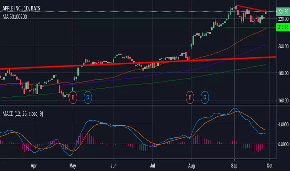
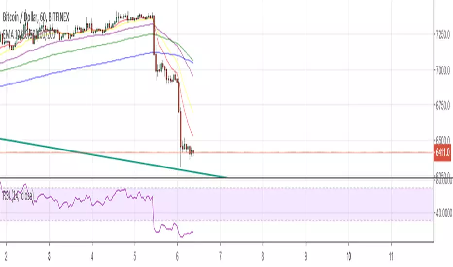
tvial/4MA Daily 20/50/100/200This indicator allows you to:
- display 4 Simple Moving Averages (SMA) at the same time with a single indicator
- display these MA in a DAILY timeframe whatever your current timeframe (4H in the example)
- settings are 20/50/100/200 but can be overridden
Simple but efficient.
Check my other indicators & strategy , they all start with "tvial/".

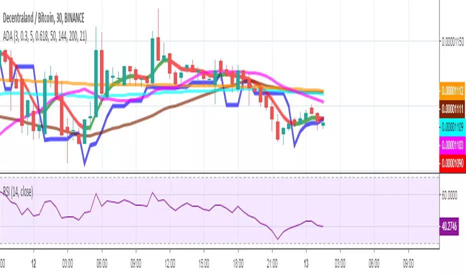
ena 21,50,144,200, tillson t3 moving average,stoploss trailingena 21,50,144,200, tillson t3 moving average,stoploss trailing
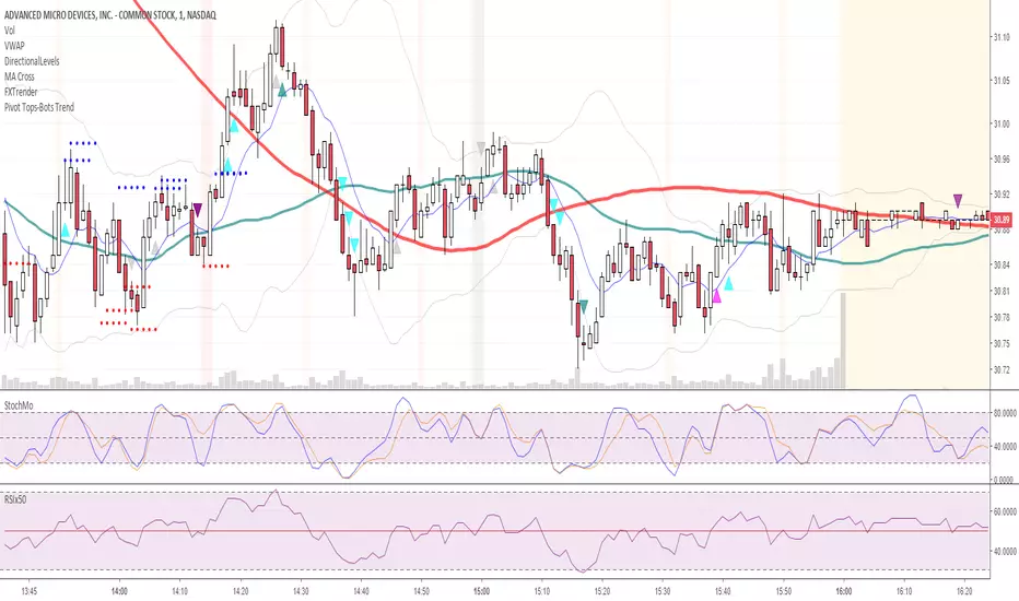
Relative Strength Index 50 LineSuper simple script that just adds a line at the 50 level for the RSI.


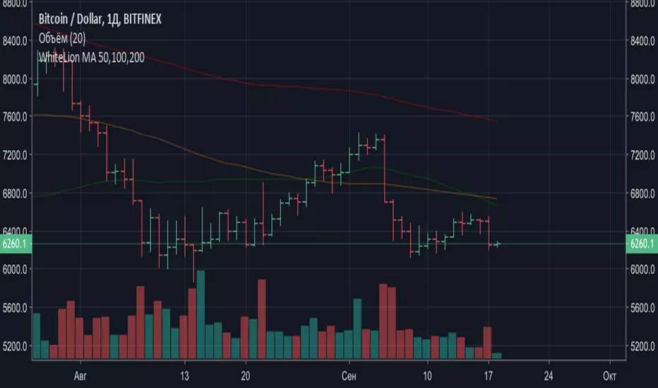
WhiteLion MA 50,100,200 v1A single indicator that includes 50 (green), 100 (orange), and 200 (red) moving averages
DFT - Dominant Cycle Period 8-50 bars - John EhlerThis is the translation of discret cosine tranform (DCT) usage by John Ehler for finding dominant cycle period (DC).
The price is first filtered to remove aliasing noise(bellow 8 bars) and trend informations(above 50 bars), then the power is computed.
The trick here is to use a normalisation against the maximum power in order to get a good frequency resolution.
Current limitation in tradingview does not allow to display all of the periods, still the DC period is plot after beeing computed based on the center of gravity algo.
The DC period can be used to tune all of the indicators based on the cycles of the markets. For instance one can use this (DC period)/2 as an input for RSI.
Hope you find this of some interrest.
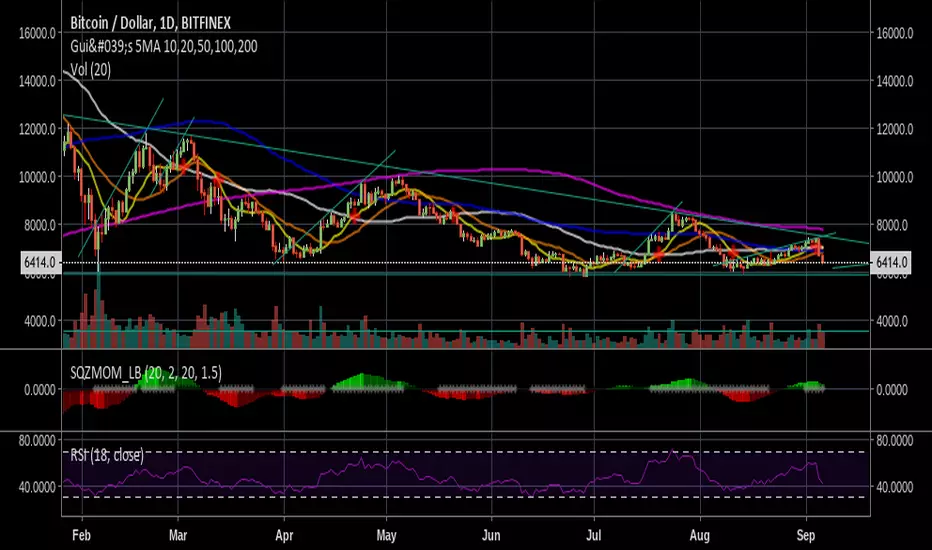
Gui's 5MA 10,20,50,100,2005 Simple Moving Averages for the 10, 20, 50, 100 and 200 day and a cross for whatever you want to read:P
Use it well! Buy high and sell low. Jk:P
Thank you!
Philakone 4EMAs + 3MAs (200+100+50)Hi guys ^^
This script combine all Philakone EMAs plus i added death and golden cross MAs which is ( 200 MA + 50 MA ) plus 100 MA
You can fully customize all moving averages MA EMA show or hide or change color or thickness and ofc 0.79% play with source code :)
BTC tip :
3BMEXA9mJMhMBJR9MR3t7othh7BijxUNW7
Thanks ^^

COLOUR CODED ULTIMATE OSCILLATOR WITH LEVELS (70/50/30)Just added 70/30/50 levels to @LazyBear 's "Color Coded UO" script.
Happy Trading!


5 Moving Average Exponential 7-15-30-50-2005 Moving Average Exponential. Crypto EMA. 7 is a fast support or resistance, 15 confirmation support or resistance. 30 Important support and resistance. 50 institutional support or resistance. 200 general trend, support and resistance.
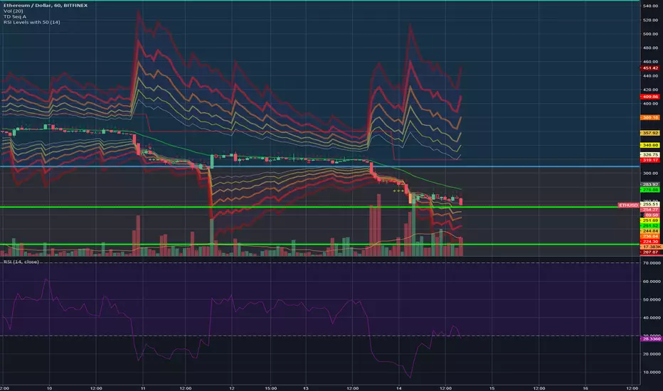
RSI Levels, 15-30 & 70-85 with 50New version of my RSI Levels, 20-30 & 70-80 considering extreme market conditions.
This version scales between 15-30 and 70-85 instead and also has RSI 50 as the middle line.