ORB 30 Alerts (ATH)Overview
ATH ORB 30m automates the Opening Range Breakout (ORB) process across multiple global sessions — Tokyo, London, and New York — and delivers clean, consolidated alerts when fresh breakouts occur.
It’s built for traders who track several tickers and want precise, non-repeating signals that reflect genuine momentum shifts, not constant noise.
How it works
The script defines a 30-minute Opening Range (ORB) for each enabled session and plots its high, low, and midpoint levels.
Every 10-minute candle close is evaluated to detect first-time crosses of those range boundaries — upward or downward.
Once a breakout triggers, that side’s alert is disabled until price returns inside the range, where the system automatically re-arms.
Multiple triggers in the same bar are batched into one combined alert, listing all symbols that broke out.
A built-in debug panel and optional chart labels visualize each trigger and re-arm event in real time.
Key features
-Multi-session ORB logic (Tokyo, London, New York)
-10-minute confirmation filter to validate breakouts
-Automatic alert re-arming when price re-enters range
-Combined per-bar alert messages (no duplicates)
-Optional on-chart labels and debug diagnostics
-Optimized for watchlists and multi-symbol scanners
Usage
Designed for day traders and momentum scalpers, this tool highlights early directional strength during market opens.
Add it to your chart, enable your preferred sessions, and set alert conditions for “ORB Breakouts (BUY),” “ORB Breakdowns (SELL),” or "Any alert() function call" You’ll receive one concise message each bar showing exactly which symbols broke out and in which direction.
DISCLAIMER:
This script is for educational and informational purposes only.
It does not constitute financial advice or a recommendation to buy or sell any security.
Always perform your own due diligence and backtesting before using any trading strategy live.
Trading involves risk; past performance does not guarantee future results.
Поиск скриптов по запросу "欧元汇率走势30天"

5x Relative Volume vs 30-Day AverageRelative Volume.
If today's volume is more than average of last 30 days volume by 5x.

Session 30 Second OR DeviationsThis indicator will plot the -4, -6, and -8 levels in color coded fashion based on session. We look for price reactions at these levels. It will plot the Asia session first 30 second candle, same with London, and New York.
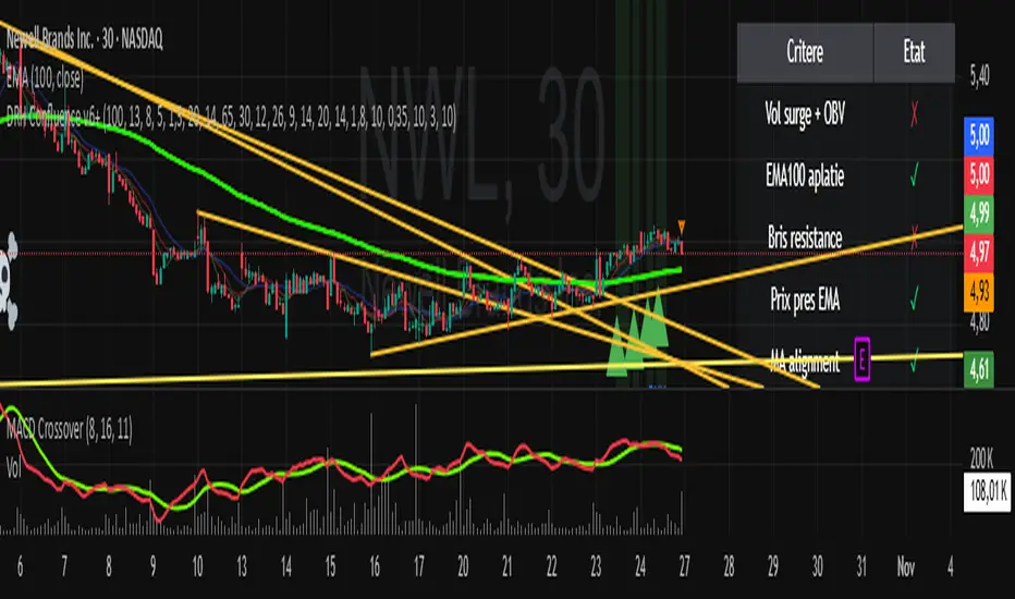
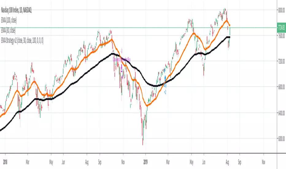
SC_Reversal Confirmation 30 minutes by Claude (Version 1)📉 When to Use
Use this setup when the stock is in a downtrend and a bullish reversal is anticipated.
🔍 Recommended Usage This model is designed for pullback phases, where the asset is declining and a reversal is expected. It helps filter out weak signals and waits for technical confirmation before triggering an entry.
✅ Entry Signal Green triangles appear only when all reversal conditions are fully met. Entry may occur slightly after the bottom, but with a reduced likelihood of false signals.
📊 Suggested Settings Apply on a 30-minute chart using a 100-period Exponential Moving Average (EMA) based on close. Recommended for Cobalt Chart 0.
--------------------------------------------------------------------------------------
ICT Largest Midnight–00:30 FVG (NY, 1 per day) — FIXEDmarks out the first and largest fvg on the 1 min chart from midnight open until 12:30 am est

BSL/SSL 8:00–9:30 ET (Daily Reset)AlexCShow you the buyside and sellside liquidity that create between 8AM EST and 9:30 AM EST

Opening Range Breakout (9:30 - 9:45 EST)Here's a Pine Script (v5) for TradingView that plots the Opening Range Breakout (ORB) lines from 9:30 AM to 9:45 AM EST on a 15-minute chart.
It draws a green line at the high of the opening range and a red line at the low, both extending through the rest of the day.

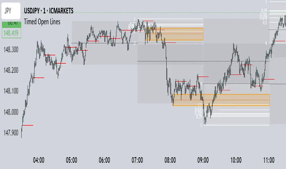
Bill Mensah - 10 / 30 / 50 Minute Open Lines Scientia maledictus sum.
Opening Macro lines extended, 10 / 30 / 50 Minute Open Lines
Daily Open Line (9:30-16:00)This indicator automatically plots a horizontal line at each day's opening price during regular trading hours (9:30 AM to 4:00 PM, US Eastern Time).
The line starts exactly at the opening bar of the day and ends at the close (16:00).
Each day, a new line is drawn, making it easy to visualize and reference the daily open price throughout the session.
Useful for intraday traders to identify key support/resistance and monitor price action relative to the open.
You can customize the color, line width, and whether to display the open price label.

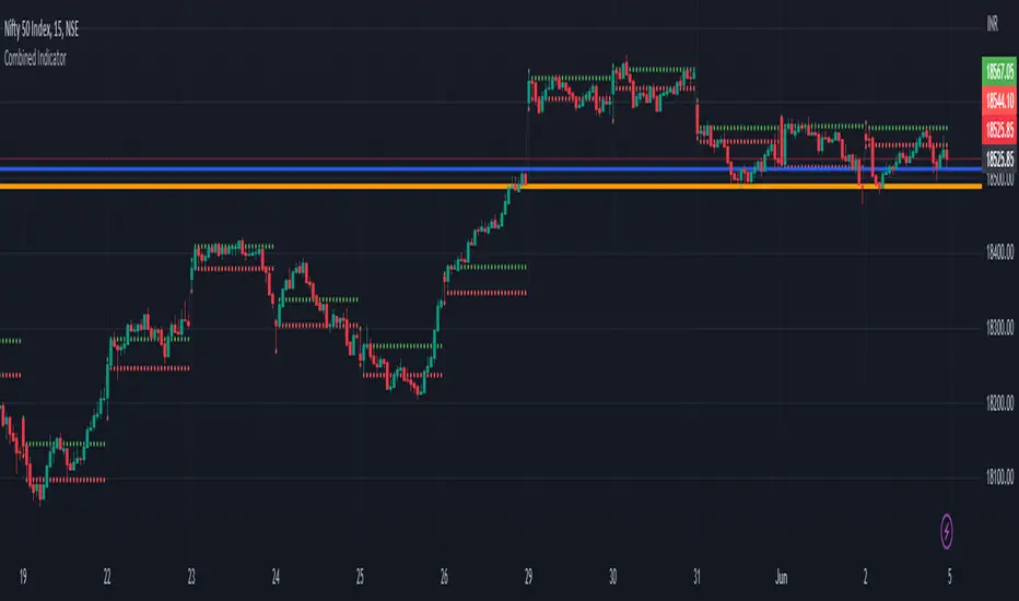
Previous Day Close and Average VWAP value, Current Day 30 min HLThe code provided is a TradingView Pine Script that creates a combined indicator consisting of two separate components:
Indicator 1: Plot Lines with VWAP
This component plots lines on the chart using two different colors and widths.
It uses a custom function f_newLine to create a new line object with a specified color and width.
It uses another custom function f_moveLine to move a line to a specific location on the chart.
The line_close line is moved to a specific date and closing price.
The line_vwap line represents the VWAP (Volume Weighted Average Price) and is plotted using the line.new function.
The VWAP calculation is performed using the typical price (average of high, low, and close) and volume.
The VWAP is plotted on the chart using the plot function.
The previous day's VWAP is also plotted and connected to the current day's VWAP with a line.
Indicator 2: 30 Min high and low breakout
This component identifies a specific time range ("0915-0945") within each trading day.
It uses the ta.valuewhen function to find the highest and lowest prices during that time range.
The highest price is stored in the high_thirtymin variable, and the lowest price is stored in the low_thirtymin variable.
These prices are plotted on the chart as circles, with green representing the high and red representing the low.
The indicator combines these two components to provide visual information about the VWAP and the high/low breakout within a specific time range. The code also includes some additional logic to handle barstate and ensure correct calculations and plotting.
Ichimoku Crypto Cloud 11-30-61A minor adjustment to the original Ichimoku Cloud, changing periods to reflect the 24/7 open market of cryptocurrency.
TENKAN: 11 - a week and a half
KIJUN: 30 - one month
SENKOU: 61 - two months
For a simpler visualization, I made the cloud limit lines and the Chikou line invisible by default.

Simple Moving Average (5,10,20,30,50,100,150,200,250)Simple Moving Average (5, 10, 20, 30, 50, 100, 150, 200, 250)
For those who want a combo of simple moving average
You can edit the color of each line when in use

14/30 SMA Price DivergencePrice divergence from 14 and 30 SMA, identify overbought + oversold conditions

CPR by Anand with PDL/PDH & Breakouts 15/30 minsThis is an enhanced version of CPR by Anand with Configurable previous day high and low and option to configure breakout lines of 15 and 30 mins.
Will be an useful tool for day traders who follows CPR tricks and breakouts.

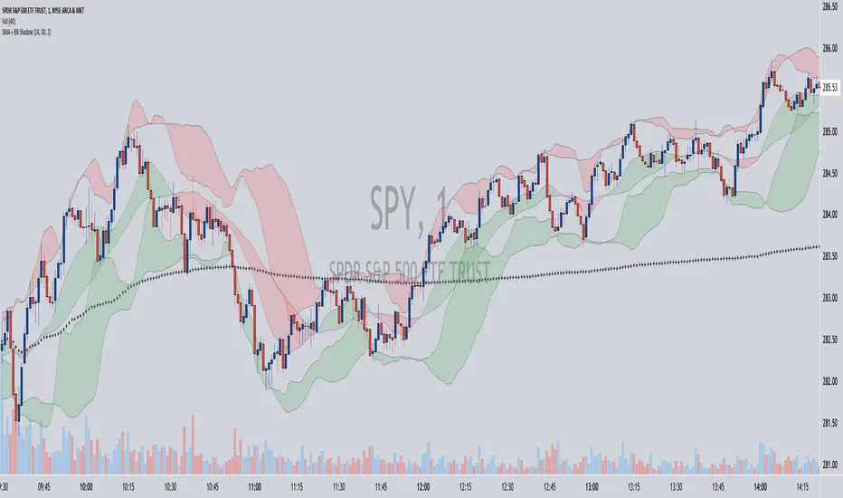
Superstock 10-30 WMA Band script I was reading Jesse Stine's Insider Buy Superstocks book, and one of the technical traits he mentioned of a superstock (read the book, seriously, very strongly recommended) was a breakout above the 30 weekly moving average. He goes on to mention that after breakout, the 10 WMA often acts as a support line where you can add to your position. This script is inspired by the visual direction of Chris Moody's slingshot system, and how it displays MA's. The skinny line is the 10 WMA and the bigger line is the 30.

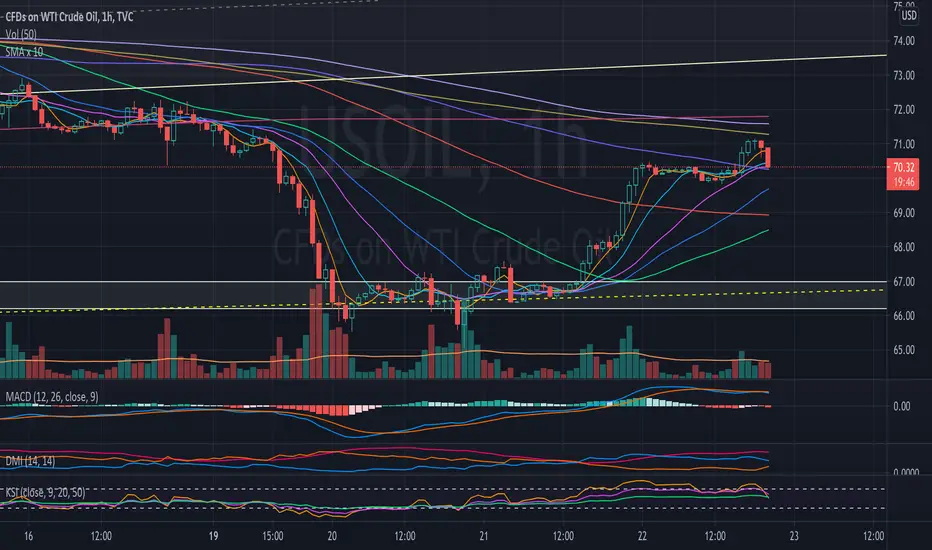
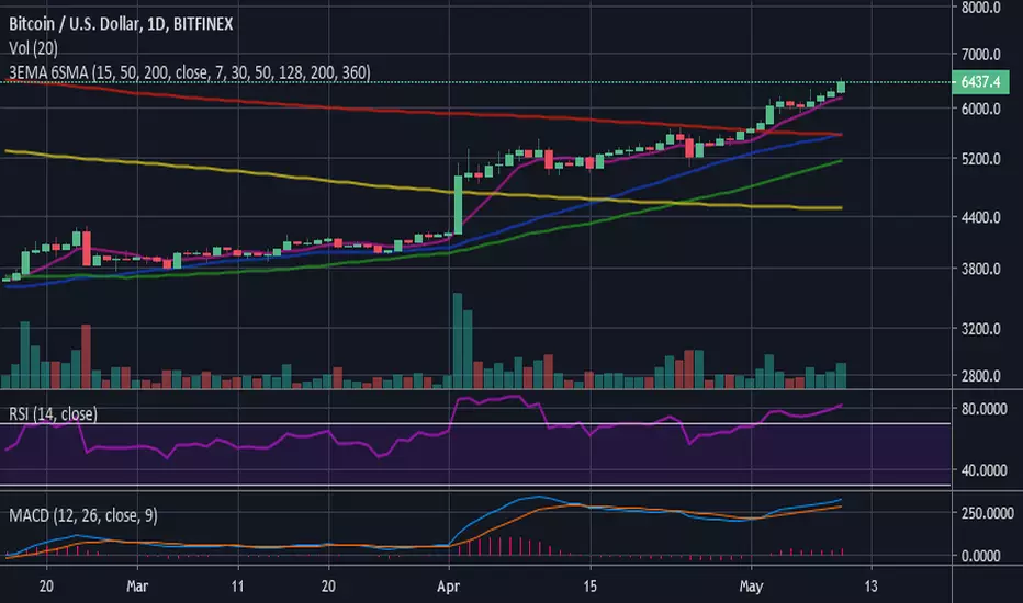
3 EMA (15-50-200) - 6 SMA (7-30-50-128-200-360)3 Moving Average Exponential - 6 Simple Moving Average . Crypto EMA - MA . 7 is a fast support or resistance, 15 confirmation support or resistance. 30 Important support and resistance . 50 institutional support or resistance. 200 institutional general trend, support and resistance , 360 general trend, support and resistance . The use of EMA or MA is according to your liking/trading plan
MA Cross 9 & 30 trend analysisvery good fro a simple trend analysis. 9 and 30 did work for me and I want to share.

EMA 21,55,100,200/SMA 30,200 by Niko
Hi stranger,
This is my script with Exponencial moving average in my scales ( 21,55,100,200) which I use, and Simple moving average (30,200).
Enjoy
