Yesterday's High v.17.07Yesterday’s High Breakout it is a trading system based on the analysis of yesterday's highs, it works in trend-following mode therefore it opens a long position at the breakout of yesterday's highs even if they occur several times in one day.
There are several methods for exiting a trade, each with its own unique strategy. The first method involves setting Take-Profit and Stop-Loss percentages, while the second utilizes a trailing-stop with a specified offset value. The third method calls for a conditional exit when the candle closes below a reference EMA.
Additionally, operational filters can be applied based on the volatility of the currency pair, such as calculating the percentage change from the opening or incorporating a gap to the previous day's high levels. These filters help to anticipate or delay entry into the market, mitigating the risk of false breakouts.
In the specific case of INJ, a 12% Take-Profit and a 1.5% Stop-Loss were set, with an activated trailing-stop percentage, TRL 1 and OFF 0.5.
To postpone entry and avoid false breakouts, a 1% gap was added to the price of yesterday's highs.
Name: Yesterday's High Breakout - Trend Follower Strategy
Author: @tumiza999
Category: Trend Follower, Breakout of Yesterday's High.
Operating mode: Spot or Futures (only long).
Trade duration: Intraday.
Timeframe: 30M, 1H, 2H, 4H
Market: Crypto
Suggested usage: Short-term trading, when the market is in trend and it is showing high volatility.
Entry: When there is a breakout of Yesterday's High.
Exit: Profit target or Trailing stop, Stop loss or Crossunder EMA.
Configuration:
- Gap to anticipate or postpone the entry before or after the identified level
- Rate of Change for Entry Condition
- Take Profit, Stop Loss and Trailing Stop
- EMA length
Backtesting:
⁃ Exchange: BINANCE
⁃ Pair: INJUSDT
⁃ Timeframe: 4H
- Treshold: 1
- Gap%: 1
- SL: 1.5
- TP:12
- TRL: 1
- OFF-TRL: 0.5
⁃ Fee: 0.075%
⁃ Slippage: 1
- Initial Capital: 10000 USDT
- Position sizing: 10% of Equity
- Start : 2018-07-26 (Out Of Sample from 2022-12-23)
- Bar magnifier: on
Credits: LucF for Pine Coders (f_security function to avoid repainting using security)
Disclaimer: Risk Management is crucial, so adjust stop loss to your comfort level. A tight stop loss can help minimise potential losses. Use at your own risk.
How you or we can improve? Source code is open so share your ideas!
Leave a comment and smash the boost button!
Thanks for your attention, happy to support the TradingView community.
Поиск скриптов по запросу "通达信+选股公式+换手率+0.5+源码"

Daily SPY PlanThe Daily SPY Plan indicator is a technical analysis tool designed to provide traders with a visual representation of price levels and take profit points for the SPY (S&P 500 ETF) on a daily timeframe. This indicator utilizes the Average True Range (ATR) to calculate projected price levels and take profit points, aiding traders in identifying potential breakout and profit-taking opportunities.
Indicator Description:
The indicator is written in Pine Script, specifically for use on the TradingView platform. It plots several levels on the price chart, each representing a potential breakout or take profit point. The levels are determined based on a fraction of the ATR added or subtracted from the closing price. The fractions used are 0.25, 0.5, 0.75, 1.0, 1.25, and 1.5 times the ATR.
The indicator distinguishes between breakout levels and take profit levels using different colors. Breakout levels, which indicate potential entry or exit points, are displayed in green, while take profit levels are shown in gray.
Key Features and Use:
ATR Calculation: The indicator calculates the Average True Range (ATR) using a specified length (default value of 14). ATR is a measure of market volatility and represents the average range between the high and low prices over a specific period.
Projected Price Levels: The indicator plots several projected price levels above and below the closing price. These levels are calculated by adding or subtracting a fraction of the ATR from the closing price. Traders can use these levels as potential breakout points or areas to set stop-loss orders.
Take Profit Points: The indicator also plots take profit points at specific levels above and below the closing price. These levels are designed to help traders identify potential areas to secure profits or partially exit their positions.
Visual Representation: The indicator utilizes step-like lines to plot the projected price levels and take profit points, providing a clear visual representation on the price chart. Traders can easily identify the relevant levels and incorporate them into their trading strategies.
Customizability: The indicator allows traders to customize the ATR length and choose whether to display Fibonacci levels (although there are no Fibonacci calculations in the provided code). These customization options enable traders to adapt the indicator to their preferred trading style and timeframe.
Limitations and Considerations:
Complementary Analysis: The Daily SPY Plan indicator should be used as a complementary tool alongside other technical analysis techniques and indicators. It provides price levels and take profit points based on ATR calculations, but it doesn't incorporate additional market factors or trading strategies.
Timeframe Suitability: The indicator is specifically designed for the daily timeframe of the SPY. Traders should consider adjusting the parameters and adapting the indicator if using it on different timeframes or instruments.
Risk Management: While the indicator suggests potential breakout and take profit points, it does not provide explicit stop-loss levels or risk management parameters. Traders should incorporate appropriate risk management techniques to protect their capital.
Conclusion:
The Daily SPY Plan indicator is a valuable technical analysis tool for traders focusing on the SPY ETF and the daily timeframe. By utilizing the ATR, it helps traders identify potential breakout levels and take profit points. However, traders should remember that this indicator is just one piece of the puzzle and should be used in conjunction with other technical analysis tools and risk management strategies to make informed trading decisions.

Regression Candle Conversion IndicatorHey everyone!
I got a pseudo-request a while ago for something like this, essentially the ability to track where another ticker would fall based on an alternative ticker.
I did create my ticker correlation reference indicator which directly looks at the correlation between 2 tickers. However, this is an indicator that operates on the same principle but is more pragmatic for trading.
What does it do?
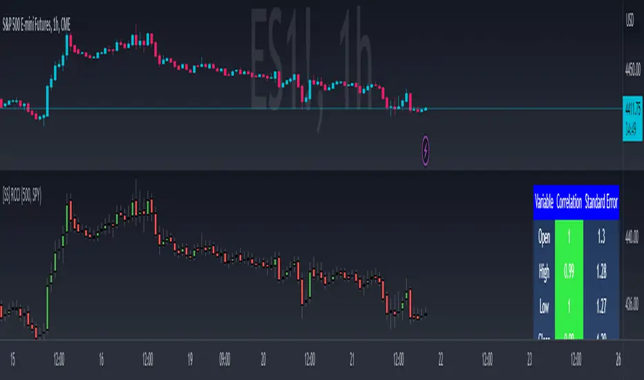
Well, in keeping with the theme of what I call my indicators, this has a title that explains exactly what it does, "Regression Candle Conversion Indicator" or "RCCI" for short. It uses simple regression to convert one ticker to another. So while you are tracking one indicator, you can see where the expected value should fall on the other.
Applications?
The big application of this for me is being able to track where SPY/QQQ or IWM is falling during overnight trading sessions. Extended trading hours close at 8 pm NYSE time. After that, you have to guess where futures prices will put the ETF version of it. This indicator will allow you to track where, theoretically, the underlying ETF ticker will fall based on the current trading behaviour.
Some other applications are just the ability to track how similar or dissimilar one stock is to the other. For example, if we wanted to trade, say, Boeing using shares of DFEN or ITA (a defence specific ETF), here is what we get:
In the chart above we can see BA as the primary chart and ITA as the RCCI converted chart. We will see 2 major things that should cause us concern.
First, there is a really poor correlation between the two tickers. This indicates that ITA may not produce the best exposure if I am directly looking for Boeing exposure.
Second, there is a wide standard error. this means that the results that the RCCI is providing may be skewed up to +/- 2 points (as indicated by the standard error chart).
Let's take a look at BA and DFEN:
In the above, we can see that the correlation is not great, but the standard error is quite low.
This means that, while this may not be the best ticker for Boeing exposure, the RCCI is able to confidently calculate the ticker within +/- 0.50 cents based on BA's underlying data.
However, its important to note that it is not advisable to really rely on these results if the correlation is less than + 0.5 or greater than -0.5.
Let's take a look at a few more examples:
Above we have BA (NYSE) vs BA (NEO TSX CAD Hedged). We can see the strong relationship and high confidence calculations.
And some others:
SPX (primary) and ES1! (secondary):
RTY and IWM:
ES1! and SPY:
Customizations:
As you can see above, it is pretty straight forward. There are 3 options:
Lookback Length: Determines the length of assessment for correlation and the regression assessment.
Manual Ticker Input: The indicator will pull the data from your current chart and compare it against a manually selected indicator. You must tell the indicator which ticker you are comparing against.
Data Table: This will show you the data table which contains the standard error assessment and the correlation assessment. These are determined by your lookback length. The lookback length is defaulted to 500.
And that's the indicator! It's pretty straight forward. Hopefully you find it helpful, especially if you track futures during overnight sessions.
Leave your comments/questions and feedback below.
Thanks for checking it out!
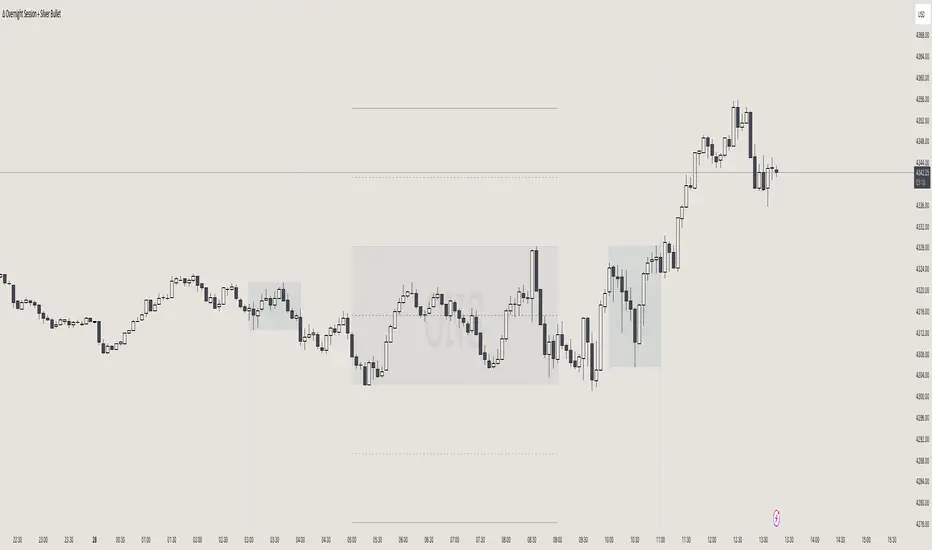
itradesize /\ Overnight Session & Silver BulletOvernight Session & Silver Bullet indicator
The indicator can be divided into two separate stuff:
ONS ( Overnight Session ) based on TCM’s ( TheCurrencyMerchant ) theory and Silver Bullet based on what ICT ( InnerCircleTrader ) is teaching to us.
Overnight Session
• ONS will be always based on Chicago 4am to 8am time according to TCM’s CME teaching.
The indicator has the option to show TSO ( Today’s session only ) which is good to have the chart not messed up by it. At this time when it comes to backtesting just turn this off to have the past ONS and SB ranges showed up on your chart.
• Mid line at the ONS range is useful to have as you are able to decide wether price is in a premium or a discount under the ONS.
If Im a buyer target is above the range, if Im a seller target is below the range.
• You are also able to have SD ( Standard Deviation ) lines for price projections. In the variety of TCM’s videos you are able to have a deeper knowledge.
• You can also extend Today’s ONS lines to the very end of the chart which could make an easier looking on the levels you eyeing with.
Silver Bullet
It’s based on New York time as ICT ( Inner Circle Trader ) is always teaching to us that we should use New York time, every time when it comes to his concepts.
Silver Bullets are always be there aiming of an opposing liquidity pool. They are working even on choppy days.
Silver Bullet hours:
• 03:00 - 04:00am NY Time
• 10:00 - 11:00am NY Time
• 02:00 - 03:00pm NY Time
SB highlighted areas could be shown as a box or a range according to your taste, with or without Start/End lines.
Both of them ca be used to form trades.
You should dig yourself into Silver Bullet ( InnerCircleTrader ) and Overnight Session ( TheCurrencyMerchant ) teachings before the use of the indicator.
Simple setups
• Silver Bullet
Look 20-30 minutes before any SB where the Buy or Sell program has started.
Where the first 1m FVG ( Fair Value Gap ) appears under the range, enter the trade.
Expect only a 5 handle move as a beginner.
1m chart is a must for these kind of FVG entries. ( 30s , 15s can also be used )
• ONS
Price is trading aggressively out of the range to take liquidity.
Once price grabbed liquidity that candle on the 3-5m could considered as on order block for the further movement.
If you are trading in the range, then the opposite side can be the target, if its out of the range and trading one sided, then use standard deviations as 0.5 is a minimum target.
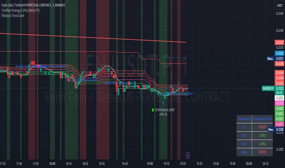
Fibonacci Trend Zone The "Fibonacci Trend Zone" indicator is a supplementary tool that helps identify the current trend based on Fibonacci zones. It utilizes Fibonacci levels (0.62, 0.705, and 0.79) to define long-term trend zones. The green zone indicates potential long trades, while the red zone suggests potential short trades. The indicator also includes the Triple Exponential Moving Average (TEMA), which helps confirm trend reversals. When the TEMA crosses the Fibonacci level of 0.5, it may signal a possible trend reversal. Use this indicator in conjunction with your primary trading strategy to make more informed trading decisions. Additionally, the indicator provides flexibility in customizing the styles, allowing you to change the color scheme or disable the display of certain elements to suit your preferences and requirements.
Индикатор "Fibonacci Trend Zone" является вспомогательным инструментом, который помогает определить текущий тренд на основе зон фибоначчи. Он использует уровни фибоначчи (0,62, 0,705 и 0,79) для определения зон долгосрочного тренда. Зеленая зона указывает на возможность лонг-сделок, а красная зона - на возможность шорт-сделок. Индикатор также включает Triple Exponential Moving Average (TEMA), который помогает подтвердить смену тренда. Когда TEMA пересекает уровень фибоначчи 0,5, это может сигнализировать о возможной смене тренда. Используйте данный индикатор в сочетании с вашей основной торговой стратегией для принятия более информированных решений. Индикатор также предоставляет гибкость в настройке стилей, позволяя вам изменить цветовую схему или отключить отображение некоторых элементов, чтобы соответствовать вашим предпочтениям и требованиям.
VWAP Trendfollow Strategy [wbburgin]This is an experimental strategy that enters long when the instrument crosses over the upper standard deviation band of a VWAP and enters short when the instrument crosses below the bottom standard deviation band of the VWAP. I have added a trend filter as well, which stops entries that are opposite to the current trend of the VWAP. The trend filter will reduce total false breakouts, thus improving the % profitable while maintaining the overall returns of the strategy. Because this is a trend-following breakout strategy, the % profitable will typically be low but the average % return will be higher. As a rule, be sure to look at the average winning trade % compared to the average losing trade %, and compare that to the % profitable to judge the effectiveness of a strategy. Factor in fees and slippage as well.
This strategy appears to work better with the lower timeframes, and I was impressed with its results. It also appears to work on a wide range of asset classes. There isn't a stop loss or take profit built-in (other than the reversal signals, which close the current trade), so I would encourage you to expand on the strategy based on your own trading parameters.
You can toggle off the bar colors and the trend filter if you so desire.
Future updates to this script (or ideas of improving on it) might include a take profit level set at one standard deviation past the current level and a stop loss level set at one standard deviation closer to the vwap from the current level - or applying a multiple to the two based off of your reward/risk ratio.
About the strategy results below: this is with commissions of 0.5 % per trade.

Vector3Library "Vector3"
Representation of 3D vectors and points.
This structure is used to pass 3D positions and directions around. It also contains functions for doing common vector operations.
Besides the functions listed below, other classes can be used to manipulate vectors and points as well.
For example the Quaternion and the Matrix4x4 classes are useful for rotating or transforming vectors and points.
___
**Reference:**
- github.com
- github.com
- github.com
- www.movable-type.co.uk
- docs.unity3d.com
- referencesource.microsoft.com
- github.com
\
new(x, y, z)
Create a new `Vector3`.
Parameters:
x (float) : `float` Property `x` value, (optional, default=na).
y (float) : `float` Property `y` value, (optional, default=na).
z (float) : `float` Property `z` value, (optional, default=na).
Returns: `Vector3` Generated new vector.
___
**Usage:**
```
.new(1.1, 1, 1)
```
from(value)
Create a new `Vector3` from a single value.
Parameters:
value (float) : `float` Properties positional value, (optional, default=na).
Returns: `Vector3` Generated new vector.
___
**Usage:**
```
.from(1.1)
```
from_Array(values, fill_na)
Create a new `Vector3` from a list of values, only reads up to the third item.
Parameters:
values (float ) : `array` Vector property values.
fill_na (float) : `float` Parameter value to replace missing indexes, (optional, defualt=na).
Returns: `Vector3` Generated new vector.
___
**Notes:**
- Supports any size of array, fills non available fields with `na`.
___
**Usage:**
```
.from_Array(array.from(1.1, fill_na=33))
.from_Array(array.from(1.1, 2, 3))
```
from_Vector2(values)
Create a new `Vector3` from a `Vector2`.
Parameters:
values (Vector2 type from RicardoSantos/CommonTypesMath/1) : `Vector2` Vector property values.
Returns: `Vector3` Generated new vector.
___
**Usage:**
```
.from:Vector2(.Vector2.new(1, 2.0))
```
___
**Notes:**
- Type `Vector2` from CommonTypesMath library.
from_Quaternion(values)
Create a new `Vector3` from a `Quaternion`'s `x, y, z` properties.
Parameters:
values (Quaternion type from RicardoSantos/CommonTypesMath/1) : `Quaternion` Vector property values.
Returns: `Vector3` Generated new vector.
___
**Usage:**
```
.from_Quaternion(.Quaternion.new(1, 2, 3, 4))
```
___
**Notes:**
- Type `Quaternion` from CommonTypesMath library.
from_String(expression, separator, fill_na)
Create a new `Vector3` from a list of values in a formated string.
Parameters:
expression (string) : `array` String with the list of vector properties.
separator (string) : `string` Separator between entries, (optional, default=`","`).
fill_na (float) : `float` Parameter value to replace missing indexes, (optional, defualt=na).
Returns: `Vector3` Generated new vector.
___
**Notes:**
- Supports any size of array, fills non available fields with `na`.
- `",,"` Empty fields will be ignored.
___
**Usage:**
```
.from_String("1.1", fill_na=33))
.from_String("(1.1,, 3)") // 1.1 , 3.0, NaN // empty field will be ignored!!
```
back()
Create a new `Vector3` object in the form `(0, 0, -1)`.
Returns: `Vector3` Generated new vector.
___
**Usage:**
```
.back()
```
front()
Create a new `Vector3` object in the form `(0, 0, 1)`.
Returns: `Vector3` Generated new vector.
___
**Usage:**
```
.front()
```
up()
Create a new `Vector3` object in the form `(0, 1, 0)`.
Returns: `Vector3` Generated new vector.
___
**Usage:**
```
.up()
```
down()
Create a new `Vector3` object in the form `(0, -1, 0)`.
Returns: `Vector3` Generated new vector.
___
**Usage:**
```
.down()
```
left()
Create a new `Vector3` object in the form `(-1, 0, 0)`.
Returns: `Vector3` Generated new vector.
___
**Usage:**
```
.left()
```
right()
Create a new `Vector3` object in the form `(1, 0, 0)`.
Returns: `Vector3` Generated new vector.
___
**Usage:**
```
.right()
```
zero()
Create a new `Vector3` object in the form `(0, 0, 0)`.
Returns: `Vector3` Generated new vector.
___
**Usage:**
```
.zero()
```
one()
Create a new `Vector3` object in the form `(1, 1, 1)`.
Returns: `Vector3` Generated new vector.
___
**Usage:**
```
.one()
```
minus_one()
Create a new `Vector3` object in the form `(-1, -1, -1)`.
Returns: `Vector3` Generated new vector.
___
**Usage:**
```
.minus_one()
```
unit_x()
Create a new `Vector3` object in the form `(1, 0, 0)`.
Returns: `Vector3` Generated new vector.
___
**Usage:**
```
.unit_x()
```
unit_y()
Create a new `Vector3` object in the form `(0, 1, 0)`.
Returns: `Vector3` Generated new vector.
___
**Usage:**
```
.unit_y()
```
unit_z()
Create a new `Vector3` object in the form `(0, 0, 1)`.
Returns: `Vector3` Generated new vector.
___
**Usage:**
```
.unit_z()
```
nan()
Create a new `Vector3` object in the form `(na, na, na)`.
Returns: `Vector3` Generated new vector.
___
**Usage:**
```
.nan()
```
random(max, min)
Generate a vector with random properties.
Parameters:
max (Vector3 type from RicardoSantos/CommonTypesMath/1) : `Vector3` Maximum defined range of the vector properties.
min (Vector3 type from RicardoSantos/CommonTypesMath/1) : `Vector3` Minimum defined range of the vector properties.
Returns: `Vector3` Generated new vector.
___
**Usage:**
```
.random(.from(math.pi), .from(-math.pi))
```
random(max)
Generate a vector with random properties (min set to 0.0).
Parameters:
max (Vector3 type from RicardoSantos/CommonTypesMath/1) : `Vector3` Maximum defined range of the vector properties.
Returns: `Vector3` Generated new vector.
___
**Usage:**
```
.random(.from(math.pi))
```
method copy(this)
Copy a existing `Vector3`
Namespace types: TMath.Vector3
Parameters:
this (Vector3 type from RicardoSantos/CommonTypesMath/1) : `Vector3` Source vector.
Returns: `Vector3` Generated new vector.
___
**Usage:**
```
a = .one().copy()
```
method i_add(this, other)
Modify a instance of a vector by adding a vector to it.
Namespace types: TMath.Vector3
Parameters:
this (Vector3 type from RicardoSantos/CommonTypesMath/1) : `Vector3` Source vector.
other (Vector3 type from RicardoSantos/CommonTypesMath/1) : `Vector3` Other Vector.
Returns: `Vector3` Updated source vector.
___
**Usage:**
```
a = .from(1) , a.i_add(.up())
```
method i_add(this, value)
Modify a instance of a vector by adding a vector to it.
Namespace types: TMath.Vector3
Parameters:
this (Vector3 type from RicardoSantos/CommonTypesMath/1) : `Vector3` Source vector.
value (float) : `float` Value.
Returns: `Vector3` Updated source vector.
___
**Usage:**
```
a = .from(1) , a.i_add(3.2)
```
method i_subtract(this, other)
Modify a instance of a vector by subtracting a vector to it.
Namespace types: TMath.Vector3
Parameters:
this (Vector3 type from RicardoSantos/CommonTypesMath/1) : `Vector3` Source vector.
other (Vector3 type from RicardoSantos/CommonTypesMath/1) : `Vector3` Other Vector.
Returns: `Vector3` Updated source vector.
___
**Usage:**
```
a = .from(1) , a.i_subtract(.down())
```
method i_subtract(this, value)
Modify a instance of a vector by subtracting a vector to it.
Namespace types: TMath.Vector3
Parameters:
this (Vector3 type from RicardoSantos/CommonTypesMath/1) : `Vector3` Source vector.
value (float) : `float` Value.
Returns: `Vector3` Updated source vector.
___
**Usage:**
```
a = .from(1) , a.i_subtract(3)
```
method i_multiply(this, other)
Modify a instance of a vector by multiplying a vector with it.
Namespace types: TMath.Vector3
Parameters:
this (Vector3 type from RicardoSantos/CommonTypesMath/1) : `Vector3` Source vector.
other (Vector3 type from RicardoSantos/CommonTypesMath/1) : `Vector3` Other Vector.
Returns: `Vector3` Updated source vector.
___
**Usage:**
```
a = .from(1) , a.i_multiply(.left())
```
method i_multiply(this, value)
Modify a instance of a vector by multiplying a vector with it.
Namespace types: TMath.Vector3
Parameters:
this (Vector3 type from RicardoSantos/CommonTypesMath/1) : `Vector3` Source vector.
value (float) : `float` value.
Returns: `Vector3` Updated source vector.
___
**Usage:**
```
a = .from(1) , a.i_multiply(3)
```
method i_divide(this, other)
Modify a instance of a vector by dividing it by another vector.
Namespace types: TMath.Vector3
Parameters:
this (Vector3 type from RicardoSantos/CommonTypesMath/1) : `Vector3` Source vector.
other (Vector3 type from RicardoSantos/CommonTypesMath/1) : `Vector3` Other Vector.
Returns: `Vector3` Updated source vector.
___
**Usage:**
```
a = .from(1) , a.i_divide(.forward())
```
method i_divide(this, value)
Modify a instance of a vector by dividing it by another vector.
Namespace types: TMath.Vector3
Parameters:
this (Vector3 type from RicardoSantos/CommonTypesMath/1) : `Vector3` Source vector.
value (float) : `float` Value.
Returns: `Vector3` Updated source vector.
___
**Usage:**
```
a = .from(1) , a.i_divide(3)
```
method i_mod(this, other)
Modify a instance of a vector by modulo assignment with another vector.
Namespace types: TMath.Vector3
Parameters:
this (Vector3 type from RicardoSantos/CommonTypesMath/1) : `Vector3` Source vector.
other (Vector3 type from RicardoSantos/CommonTypesMath/1) : `Vector3` Other Vector.
Returns: `Vector3` Updated source vector.
___
**Usage:**
```
a = .from(1) , a.i_mod(.back())
```
method i_mod(this, value)
Modify a instance of a vector by modulo assignment with another vector.
Namespace types: TMath.Vector3
Parameters:
this (Vector3 type from RicardoSantos/CommonTypesMath/1) : `Vector3` Source vector.
value (float) : `float` Value.
Returns: `Vector3` Updated source vector.
___
**Usage:**
```
a = .from(1) , a.i_mod(3)
```
method i_pow(this, exponent)
Modify a instance of a vector by modulo assignment with another vector.
Namespace types: TMath.Vector3
Parameters:
this (Vector3 type from RicardoSantos/CommonTypesMath/1) : `Vector3` Source vector.
exponent (Vector3 type from RicardoSantos/CommonTypesMath/1) : `Vector3` Exponent Vector.
Returns: `Vector3` Updated source vector.
___
**Usage:**
```
a = .from(1) , a.i_pow(.up())
```
method i_pow(this, exponent)
Modify a instance of a vector by modulo assignment with another vector.
Namespace types: TMath.Vector3
Parameters:
this (Vector3 type from RicardoSantos/CommonTypesMath/1) : `Vector3` Source vector.
exponent (float) : `float` Exponent Value.
Returns: `Vector3` Updated source vector.
___
**Usage:**
```
a = .from(1) , a.i_pow(2)
```
method length_squared(this)
Squared length of the vector.
Namespace types: TMath.Vector3
Parameters:
this (Vector3 type from RicardoSantos/CommonTypesMath/1)
Returns: `float` The squared length of this vector.
___
**Usage:**
```
a = .one().length_squared()
```
method magnitude_squared(this)
Squared magnitude of the vector.
Namespace types: TMath.Vector3
Parameters:
this (Vector3 type from RicardoSantos/CommonTypesMath/1) : `Vector3` Source vector.
Returns: `float` The length squared of this vector.
___
**Usage:**
```
a = .one().magnitude_squared()
```
method length(this)
Length of the vector.
Namespace types: TMath.Vector3
Parameters:
this (Vector3 type from RicardoSantos/CommonTypesMath/1) : `Vector3` Source vector.
Returns: `float` The length of this vector.
___
**Usage:**
```
a = .one().length()
```
method magnitude(this)
Magnitude of the vector.
Namespace types: TMath.Vector3
Parameters:
this (Vector3 type from RicardoSantos/CommonTypesMath/1) : `Vector3` Source vector.
Returns: `float` The Length of this vector.
___
**Usage:**
```
a = .one().magnitude()
```
method normalize(this, magnitude, eps)
Normalize a vector with a magnitude of 1(optional).
Namespace types: TMath.Vector3
Parameters:
this (Vector3 type from RicardoSantos/CommonTypesMath/1) : `Vector3` Source vector.
magnitude (float) : `float` Value to manipulate the magnitude of normalization, (optional, default=1.0).
eps (float)
Returns: `Vector3` Generated new vector.
___
**Usage:**
```
a = .new(33, 50, 100).normalize() // (x=0.283, y=0.429, z=0.858)
a = .new(33, 50, 100).normalize(2) // (x=0.142, y=0.214, z=0.429)
```
method to_String(this, precision)
Converts source vector to a string format, in the form `"(x, y, z)"`.
Namespace types: TMath.Vector3
Parameters:
this (Vector3 type from RicardoSantos/CommonTypesMath/1) : `Vector3` Source vector.
precision (string) : `string` Precision format to apply to values (optional, default='').
Returns: `string` Formated string in a `"(x, y, z)"` format.
___
**Usage:**
```
a = .one().to_String("#.###")
```
method to_Array(this)
Converts source vector to a array format.
Namespace types: TMath.Vector3
Parameters:
this (Vector3 type from RicardoSantos/CommonTypesMath/1) : `Vector3` Source vector.
Returns: `array` List of the vector properties.
___
**Usage:**
```
a = .new(1, 2, 3).to_Array()
```
method to_Vector2(this)
Converts source vector to a Vector2 in the form `x, y`.
Namespace types: TMath.Vector3
Parameters:
this (Vector3 type from RicardoSantos/CommonTypesMath/1) : `Vector3` Source vector.
Returns: `Vector2` Generated new vector.
___
**Usage:**
```
a = .from(1).to_Vector2()
```
method to_Quaternion(this, w)
Converts source vector to a Quaternion in the form `x, y, z, w`.
Namespace types: TMath.Vector3
Parameters:
this (Vector3 type from RicardoSantos/CommonTypesMath/1) : `Vector3` Sorce vector.
w (float) : `float` Property of `w` new value.
Returns: `Quaternion` Generated new vector.
___
**Usage:**
```
a = .from(1).to_Quaternion(w=1)
```
method add(this, other)
Add a vector to source vector.
Namespace types: TMath.Vector3
Parameters:
this (Vector3 type from RicardoSantos/CommonTypesMath/1) : `Vector3` Source vector.
other (Vector3 type from RicardoSantos/CommonTypesMath/1) : `Vector3` Other vector.
Returns: `Vector3` Generated new vector.
___
**Usage:**
```
a = .from(1).add(.unit_z())
```
method add(this, value)
Add a value to each property of the vector.
Namespace types: TMath.Vector3
Parameters:
this (Vector3 type from RicardoSantos/CommonTypesMath/1) : `Vector3` Source vector.
value (float) : `float` Value.
Returns: `Vector3` Generated new vector.
___
**Usage:**
```
a = .from(1).add(2.0)
```
add(value, other)
Add each property of a vector to a base value as a new vector.
Parameters:
value (float) : `float` Value.
other (Vector3 type from RicardoSantos/CommonTypesMath/1) : `Vector3` Vector.
Returns: `Vector3` Generated new vector.
___
**Usage:**
```
a = .from(2) , b = .add(1.0, a)
```
method subtract(this, other)
Subtract vector from source vector.
Namespace types: TMath.Vector3
Parameters:
this (Vector3 type from RicardoSantos/CommonTypesMath/1) : `Vector3` Source vector.
other (Vector3 type from RicardoSantos/CommonTypesMath/1) : `Vector3` Other vector.
Returns: `Vector3` Generated new vector.
___
**Usage:**
```
a = .from(1).subtract(.left())
```
method subtract(this, value)
Subtract a value from each property in source vector.
Namespace types: TMath.Vector3
Parameters:
this (Vector3 type from RicardoSantos/CommonTypesMath/1) : `Vector3` Source vector.
value (float) : `float` Value.
Returns: `Vector3` Generated new vector.
___
**Usage:**
```
a = .from(1).subtract(2.0)
```
subtract(value, other)
Subtract each property in a vector from a base value and create a new vector.
Parameters:
value (float) : `float` Value.
other (Vector3 type from RicardoSantos/CommonTypesMath/1) : `Vector3` Vector.
Returns: `Vector3` Generated new vector.
___
**Usage:**
```
a = .subtract(1.0, .right())
```
method multiply(this, other)
Multiply a vector by another.
Namespace types: TMath.Vector3
Parameters:
this (Vector3 type from RicardoSantos/CommonTypesMath/1) : `Vector3` Source vector.
other (Vector3 type from RicardoSantos/CommonTypesMath/1) : `Vector3` Other vector.
Returns: `Vector3` Generated new vector.
___
**Usage:**
```
a = .from(1).multiply(.up())
```
method multiply(this, value)
Multiply each element in source vector with a value.
Namespace types: TMath.Vector3
Parameters:
this (Vector3 type from RicardoSantos/CommonTypesMath/1) : `Vector3` Source vector.
value (float) : `float` Value.
Returns: `Vector3` Generated new vector.
___
**Usage:**
```
a = .from(1).multiply(2.0)
```
multiply(value, other)
Multiply a value with each property in a vector and create a new vector.
Parameters:
value (float) : `float` Value.
other (Vector3 type from RicardoSantos/CommonTypesMath/1) : `Vector3` Vector.
Returns: `Vector3` Generated new vector.
___
**Usage:**
```
a = .multiply(1.0, .new(1, 2, 1))
```
method divide(this, other)
Divide a vector by another.
Namespace types: TMath.Vector3
Parameters:
this (Vector3 type from RicardoSantos/CommonTypesMath/1) : `Vector3` Source vector.
other (Vector3 type from RicardoSantos/CommonTypesMath/1) : `Vector3` Other vector.
Returns: `Vector3` Generated new vector.
___
**Usage:**
```
a = .from(1).divide(.from(2))
```
method divide(this, value)
Divide each property in a vector by a value.
Namespace types: TMath.Vector3
Parameters:
this (Vector3 type from RicardoSantos/CommonTypesMath/1) : `Vector3` Source vector.
value (float) : `float` Value.
Returns: `Vector3` Generated new vector.
___
**Usage:**
```
a = .from(1).divide(2.0)
```
divide(value, other)
Divide a base value by each property in a vector and create a new vector.
Parameters:
value (float) : `float` Value.
other (Vector3 type from RicardoSantos/CommonTypesMath/1) : `Vector3` Vector.
Returns: `Vector3` Generated new vector.
___
**Usage:**
```
a = .divide(1.0, .from(2))
```
method mod(this, other)
Modulo a vector by another.
Namespace types: TMath.Vector3
Parameters:
this (Vector3 type from RicardoSantos/CommonTypesMath/1) : `Vector3` Source vector.
other (Vector3 type from RicardoSantos/CommonTypesMath/1) : `Vector3` Other vector.
Returns: `Vector3` Generated new vector.
___
**Usage:**
```
a = .from(1).mod(.from(2))
```
method mod(this, value)
Modulo each property in a vector by a value.
Namespace types: TMath.Vector3
Parameters:
this (Vector3 type from RicardoSantos/CommonTypesMath/1) : `Vector3` Source vector.
value (float) : `float` Value.
Returns: `Vector3` Generated new vector.
___
**Usage:**
```
a = .from(1).mod(2.0)
```
mod(value, other)
Modulo a base value by each property in a vector and create a new vector.
Parameters:
value (float) : `float` Value.
other (Vector3 type from RicardoSantos/CommonTypesMath/1) : `Vector3` Vector.
Returns: `Vector3` Generated new vector.
___
**Usage:**
```
a = .mod(1.0, .from(2))
```
method negate(this)
Negate a vector in the form `(zero - this)`.
Namespace types: TMath.Vector3
Parameters:
this (Vector3 type from RicardoSantos/CommonTypesMath/1) : `Vector3` Source vector.
Returns: `Vector3` Generated new vector.
___
**Usage:**
```
a = .one().negate()
```
method pow(this, other)
Modulo a vector by another.
Namespace types: TMath.Vector3
Parameters:
this (Vector3 type from RicardoSantos/CommonTypesMath/1) : `Vector3` Source vector.
other (Vector3 type from RicardoSantos/CommonTypesMath/1) : `Vector3` Other vector.
Returns: `Vector3` Generated new vector.
___
**Usage:**
```
a = .from(2).pow(.from(3))
```
method pow(this, exponent)
Raise the vector elements by a exponent.
Namespace types: TMath.Vector3
Parameters:
this (Vector3 type from RicardoSantos/CommonTypesMath/1) : `Vector3` Source vector.
exponent (float) : `float` The exponent to raise the vector by.
Returns: `Vector3` Generated new vector.
___
**Usage:**
```
a = .from(1).pow(2.0)
```
pow(value, exponent)
Raise value into a vector raised by the elements in exponent vector.
Parameters:
value (float) : `float` Base value.
exponent (Vector3 type from RicardoSantos/CommonTypesMath/1) : `Vector3` The exponent to raise the vector of base value by.
Returns: `Vector3` Generated new vector.
___
**Usage:**
```
a = .pow(1.0, .from(2))
```
method sqrt(this)
Square root of the elements in a vector.
Namespace types: TMath.Vector3
Parameters:
this (Vector3 type from RicardoSantos/CommonTypesMath/1) : `Vector3` Source vector.
Returns: `Vector3` Generated new vector.
___
**Usage:**
```
a = .from(1).sqrt()
```
method abs(this)
Absolute properties of the vector.
Namespace types: TMath.Vector3
Parameters:
this (Vector3 type from RicardoSantos/CommonTypesMath/1) : `Vector3` Source vector.
Returns: `Vector3` Generated new vector.
___
**Usage:**
```
a = .from(1).abs()
```
method max(this)
Highest property of the vector.
Namespace types: TMath.Vector3
Parameters:
this (Vector3 type from RicardoSantos/CommonTypesMath/1) : `Vector3` Source vector.
Returns: `float` Highest value amongst the vector properties.
___
**Usage:**
```
a = .new(1, 2, 3).max()
```
method min(this)
Lowest element of the vector.
Namespace types: TMath.Vector3
Parameters:
this (Vector3 type from RicardoSantos/CommonTypesMath/1) : `Vector3` Source vector.
Returns: `float` Lowest values amongst the vector properties.
___
**Usage:**
```
a = .new(1, 2, 3).min()
```
method floor(this)
Floor of vector a.
Namespace types: TMath.Vector3
Parameters:
this (Vector3 type from RicardoSantos/CommonTypesMath/1) : `Vector3` Source vector.
Returns: `Vector3` Generated new vector.
___
**Usage:**
```
a = .new(1.33, 1.66, 1.99).floor()
```
method ceil(this)
Ceil of vector a.
Namespace types: TMath.Vector3
Parameters:
this (Vector3 type from RicardoSantos/CommonTypesMath/1) : `Vector3` Source vector.
Returns: `Vector3` Generated new vector.
___
**Usage:**
```
a = .new(1.33, 1.66, 1.99).ceil()
```
method round(this)
Round of vector elements.
Namespace types: TMath.Vector3
Parameters:
this (Vector3 type from RicardoSantos/CommonTypesMath/1) : `Vector3` Source vector.
Returns: `Vector3` Generated new vector.
___
**Usage:**
```
a = .new(1.33, 1.66, 1.99).round()
```
method round(this, precision)
Round of vector elements to n digits.
Namespace types: TMath.Vector3
Parameters:
this (Vector3 type from RicardoSantos/CommonTypesMath/1) : `Vector3` Source vector.
precision (int) : `int` Number of digits to round the vector elements.
Returns: `Vector3` Generated new vector.
___
**Usage:**
```
a = .new(1.33, 1.66, 1.99).round(1) // 1.3, 1.7, 2
```
method fractional(this)
Fractional parts of vector.
Namespace types: TMath.Vector3
Parameters:
this (Vector3 type from RicardoSantos/CommonTypesMath/1) : `Vector3` Source vector.
Returns: `Vector3` Generated new vector.
___
**Usage:**
```
a = .from(1.337).fractional() // 0.337
```
method dot_product(this, other)
Dot product of two vectors.
Namespace types: TMath.Vector3
Parameters:
this (Vector3 type from RicardoSantos/CommonTypesMath/1) : `Vector3` Source vector.
other (Vector3 type from RicardoSantos/CommonTypesMath/1) : `Vector3` Other vector.
Returns: `float` Dot product.
___
**Usage:**
```
a = .from(2).dot_product(.left())
```
method cross_product(this, other)
Cross product of two vectors.
Namespace types: TMath.Vector3
Parameters:
this (Vector3 type from RicardoSantos/CommonTypesMath/1) : `Vector3` Source vector.
other (Vector3 type from RicardoSantos/CommonTypesMath/1) : `Vector3` Other vector.
Returns: `Vector3` Generated new vector.
___
**Usage:**
```
a = .from(1).cross_produc(.right())
```
method scale(this, scalar)
Scale vector by a scalar value.
Namespace types: TMath.Vector3
Parameters:
this (Vector3 type from RicardoSantos/CommonTypesMath/1) : `Vector3` Source vector.
scalar (float) : `float` Value to scale the the vector by.
Returns: `Vector3` Generated new vector.
___
**Usage:**
```
a = .from(1).scale(2)
```
method rescale(this, magnitude)
Rescale a vector to a new magnitude.
Namespace types: TMath.Vector3
Parameters:
this (Vector3 type from RicardoSantos/CommonTypesMath/1) : `Vector3` Source vector.
magnitude (float) : `float` Value to manipulate the magnitude of normalization.
Returns: `Vector3` Generated new vector.
___
**Usage:**
```
a = .from(20).rescale(1)
```
method equals(this, other)
Compares two vectors.
Namespace types: TMath.Vector3
Parameters:
this (Vector3 type from RicardoSantos/CommonTypesMath/1) : `Vector3` Source vector.
other (Vector3 type from RicardoSantos/CommonTypesMath/1) : `Vector3` Other vector.
Returns: `Vector3` Generated new vector.
___
**Usage:**
```
a = .from(1).equals(.one())
```
method sin(this)
Sine of vector.
Namespace types: TMath.Vector3
Parameters:
this (Vector3 type from RicardoSantos/CommonTypesMath/1) : `Vector3` Source vector.
Returns: `Vector3` Generated new vector.
___
**Usage:**
```
a = .from(1).sin()
```
method cos(this)
Cosine of vector.
Namespace types: TMath.Vector3
Parameters:
this (Vector3 type from RicardoSantos/CommonTypesMath/1) : `Vector3` Source vector.
Returns: `Vector3` Generated new vector.
___
**Usage:**
```
a = .from(1).cos()
```
method tan(this)
Tangent of vector.
Namespace types: TMath.Vector3
Parameters:
this (Vector3 type from RicardoSantos/CommonTypesMath/1) : `Vector3` Source vector.
Returns: `Vector3` Generated new vector.
___
**Usage:**
```
a = .from(1).tan()
```
vmax(a, b)
Highest elements of the properties from two vectors.
Parameters:
a (Vector3 type from RicardoSantos/CommonTypesMath/1) : `Vector3` Vector.
b (Vector3 type from RicardoSantos/CommonTypesMath/1) : `Vector3` Vector.
Returns: `Vector3` Generated new vector.
___
**Usage:**
```
a = .vmax(.one(), .from(2))
```
vmax(a, b, c)
Highest elements of the properties from three vectors.
Parameters:
a (Vector3 type from RicardoSantos/CommonTypesMath/1) : `Vector3` Vector.
b (Vector3 type from RicardoSantos/CommonTypesMath/1) : `Vector3` Vector.
c (Vector3 type from RicardoSantos/CommonTypesMath/1) : `Vector3` Vector.
Returns: `Vector3` Generated new vector.
___
**Usage:**
```
a = .vmax(.new(0.1, 2.5, 3.4), .from(2), .from(3))
```
vmin(a, b)
Lowest elements of the properties from two vectors.
Parameters:
a (Vector3 type from RicardoSantos/CommonTypesMath/1) : `Vector3` Vector.
b (Vector3 type from RicardoSantos/CommonTypesMath/1) : `Vector3` Vector.
Returns: `Vector3` Generated new vector.
___
**Usage:**
```
a = .vmin(.one(), .from(2))
```
vmin(a, b, c)
Lowest elements of the properties from three vectors.
Parameters:
a (Vector3 type from RicardoSantos/CommonTypesMath/1) : `Vector3` Vector.
b (Vector3 type from RicardoSantos/CommonTypesMath/1) : `Vector3` Vector.
c (Vector3 type from RicardoSantos/CommonTypesMath/1) : `Vector3` Vector.
Returns: `Vector3` Generated new vector.
___
**Usage:**
```
a = .vmin(.one(), .from(2), .new(3.3, 2.2, 0.5))
```
distance(a, b)
Distance between vector `a` and `b`.
Parameters:
a (Vector3 type from RicardoSantos/CommonTypesMath/1) : `Vector3` Source vector.
b (Vector3 type from RicardoSantos/CommonTypesMath/1) : `Vector3` Target vector.
Returns: `Vector3` Generated new vector.
___
**Usage:**
```
a = distance(.from(3), .unit_z())
```
clamp(a, min, max)
Restrict a vector between a min and max vector.
Parameters:
a (Vector3 type from RicardoSantos/CommonTypesMath/1) : `Vector3` Source vector.
min (Vector3 type from RicardoSantos/CommonTypesMath/1) : `Vector3` Minimum boundary vector.
max (Vector3 type from RicardoSantos/CommonTypesMath/1) : `Vector3` Maximum boundary vector.
Returns: `Vector3` Generated new vector.
___
**Usage:**
```
a = .clamp(a=.new(2.9, 1.5, 3.9), min=.from(2), max=.new(2.5, 3.0, 3.5))
```
clamp_magnitude(a, radius)
Vector with its magnitude clamped to a radius.
Parameters:
a (Vector3 type from RicardoSantos/CommonTypesMath/1) : `Vector3` Source vector.object, vector with properties that should be restricted to a radius.
radius (float) : `float` Maximum radius to restrict magnitude of vector.
Returns: `Vector3` Generated new vector.
___
**Usage:**
```
a = .clamp_magnitude(.from(21), 7)
```
lerp_unclamped(a, b, rate)
`Unclamped` linearly interpolates between provided vectors by a rate.
Parameters:
a (Vector3 type from RicardoSantos/CommonTypesMath/1) : `Vector3` Source vector.
b (Vector3 type from RicardoSantos/CommonTypesMath/1) : `Vector3` Target vector.
rate (float) : `float` Rate of interpolation, range(0 > 1) where 0 == source vector and 1 == target vector.
Returns: `Vector3` Generated new vector.
___
**Usage:**
```
a = .lerp_unclamped(.from(1), .from(2), 1.2)
```
lerp(a, b, rate)
Linearly interpolates between provided vectors by a rate.
Parameters:
a (Vector3 type from RicardoSantos/CommonTypesMath/1) : `Vector3` Source vector.
b (Vector3 type from RicardoSantos/CommonTypesMath/1) : `Vector3` Target vector.
rate (float) : `float` Rate of interpolation, range(0 > 1) where 0 == source vector and 1 == target vector.
Returns: `Vector3` Generated new vector.
___
**Usage:**
```
a = lerp(.one(), .from(2), 0.2)
```
herp(start, start_tangent, end, end_tangent, rate)
Hermite curve interpolation between provided vectors.
Parameters:
start (Vector3 type from RicardoSantos/CommonTypesMath/1) : `Vector3` Start vector.
start_tangent (Vector3 type from RicardoSantos/CommonTypesMath/1) : `Vector3` Start vector tangent.
end (Vector3 type from RicardoSantos/CommonTypesMath/1) : `Vector3` End vector.
end_tangent (Vector3 type from RicardoSantos/CommonTypesMath/1) : `Vector3` End vector tangent.
rate (int) : `float` Rate of the movement from `start` to `end` to get position, should be range(0 > 1).
Returns: `Vector3` Generated new vector.
___
**Usage:**
```
s = .new(0, 0, 0) , st = .new(0, 1, 1)
e = .new(1, 2, 2) , et = .new(-1, -1, 3)
h = .herp(s, st, e, et, 0.3)
```
___
**Reference:** en.m.wikibooks.org
herp_2(a, b, rate)
Hermite curve interpolation between provided vectors.
Parameters:
a (Vector3 type from RicardoSantos/CommonTypesMath/1) : `Vector3` Source vector.
b (Vector3 type from RicardoSantos/CommonTypesMath/1) : `Vector3` Target vector.
rate (Vector3 type from RicardoSantos/CommonTypesMath/1) : `Vector3` Rate of the movement per component from `start` to `end` to get position, should be range(0 > 1).
Returns: `Vector3` Generated new vector.
___
**Usage:**
```
h = .herp_2(.one(), .new(0.1, 3, 2), 0.6)
```
noise(a)
3D Noise based on Morgan McGuire @morgan3d
Parameters:
a (Vector3 type from RicardoSantos/CommonTypesMath/1) : `Vector3` Source vector.
Returns: `Vector3` Generated new vector.
___
**Usage:**
```
a = noise(.one())
```
___
**Reference:**
- thebookofshaders.com
- www.shadertoy.com
rotate(a, axis, angle)
Rotate a vector around a axis.
Parameters:
a (Vector3 type from RicardoSantos/CommonTypesMath/1) : `Vector3` Source vector.
axis (string) : `string` The plane to rotate around, `option="x", "y", "z"`.
angle (float) : `float` Angle in radians.
Returns: `Vector3` Generated new vector.
___
**Usage:**
```
a = .rotate(.from(3), 'y', math.toradians(45.0))
```
rotate_x(a, angle)
Rotate a vector on a fixed `x`.
Parameters:
a (Vector3 type from RicardoSantos/CommonTypesMath/1) : `Vector3` Source vector.
angle (float) : `float` Angle in radians.
Returns: `Vector3` Generated new vector.
___
**Usage:**
```
a = .rotate_x(.from(3), math.toradians(90.0))
```
rotate_y(a, angle)
Rotate a vector on a fixed `y`.
Parameters:
a (Vector3 type from RicardoSantos/CommonTypesMath/1) : `Vector3` Source vector.
angle (float) : `float` Angle in radians.
Returns: `Vector3` Generated new vector.
___
**Usage:**
```
a = .rotate_y(.from(3), math.toradians(90.0))
```
rotate_yaw_pitch(a, yaw, pitch)
Rotate a vector by yaw and pitch values.
Parameters:
a (Vector3 type from RicardoSantos/CommonTypesMath/1) : `Vector3` Source vector.
yaw (float) : `float` Angle in radians.
pitch (float) : `float` Angle in radians.
Returns: `Vector3` Generated new vector.
___
**Usage:**
```
a = .rotate_yaw_pitch(.from(3), math.toradians(90.0), math.toradians(45.0))
```
project(a, normal, eps)
Project a vector off a plane defined by a normal.
Parameters:
a (Vector3 type from RicardoSantos/CommonTypesMath/1) : `Vector3` Source vector.
normal (Vector3 type from RicardoSantos/CommonTypesMath/1) : `Vector3` The normal of the surface being reflected off.
eps (float) : `float` Minimum resolution to void division by zero (default=0.000001).
Returns: `Vector3` Generated new vector.
___
**Usage:**
```
a = .project(.one(), .down())
```
project_on_plane(a, normal, eps)
Projects a vector onto a plane defined by a normal orthogonal to the plane.
Parameters:
a (Vector3 type from RicardoSantos/CommonTypesMath/1) : `Vector3` Source vector.
normal (Vector3 type from RicardoSantos/CommonTypesMath/1) : `Vector3` The normal of the surface being reflected off.
eps (float) : `float` Minimum resolution to void division by zero (default=0.000001).
Returns: `Vector3` Generated new vector.
___
**Usage:**
```
a = .project_on_plane(.one(), .left())
```
project_to_2d(a, camera_position, camera_target)
Project a vector onto a two dimensions plane.
Parameters:
a (Vector3 type from RicardoSantos/CommonTypesMath/1) : `Vector3` Source vector.
camera_position (Vector3 type from RicardoSantos/CommonTypesMath/1) : `Vector3` Camera position.
camera_target (Vector3 type from RicardoSantos/CommonTypesMath/1) : `Vector3` Camera target plane position.
Returns: `Vector2` Generated new vector.
___
**Usage:**
```
a = .project_to_2d(.one(), .new(2, 2, 3), .zero())
```
reflect(a, normal)
Reflects a vector off a plane defined by a normal.
Parameters:
a (Vector3 type from RicardoSantos/CommonTypesMath/1) : `Vector3` Source vector.
normal (Vector3 type from RicardoSantos/CommonTypesMath/1) : `Vector3` The normal of the surface being reflected off.
Returns: `Vector3` Generated new vector.
___
**Usage:**
```
a = .reflect(.one(), .right())
```
angle(a, b, eps)
Angle in degrees between two vectors.
Parameters:
a (Vector3 type from RicardoSantos/CommonTypesMath/1) : `Vector3` Source vector.
b (Vector3 type from RicardoSantos/CommonTypesMath/1) : `Vector3` Target vector.
eps (float) : `float` Minimum resolution to void division by zero (default=1.0e-15).
Returns: `float` Angle value in degrees.
___
**Usage:**
```
a = .angle(.one(), .up())
```
angle_signed(a, b, axis)
Signed angle in degrees between two vectors.
Parameters:
a (Vector3 type from RicardoSantos/CommonTypesMath/1) : `Vector3` Source vector.
b (Vector3 type from RicardoSantos/CommonTypesMath/1) : `Vector3` Target vector.
axis (Vector3 type from RicardoSantos/CommonTypesMath/1) : `Vector3` Axis vector.
Returns: `float` Angle value in degrees.
___
**Usage:**
```
a = .angle_signed(.one(), .left(), .down())
```
___
**Notes:**
- The smaller of the two possible angles between the two vectors is returned, therefore the result will never
be greater than 180 degrees or smaller than -180 degrees.
- If you imagine the from and to vectors as lines on a piece of paper, both originating from the same point,
then the /axis/ vector would point up out of the paper.
- The measured angle between the two vectors would be positive in a clockwise direction and negative in an
anti-clockwise direction.
___
**Reference:**
- github.com
angle2d(a, b)
2D angle between two vectors.
Parameters:
a (Vector3 type from RicardoSantos/CommonTypesMath/1) : `Vector3` Source vector.
b (Vector3 type from RicardoSantos/CommonTypesMath/1) : `Vector3` Target vector.
Returns: `float` Angle value in degrees.
___
**Usage:**
```
a = .angle2d(.one(), .left())
```
transform_Matrix(a, M)
Transforms a vector by the given matrix.
Parameters:
a (Vector3 type from RicardoSantos/CommonTypesMath/1) : `Vector3` Source vector.
M (matrix) : `matrix` A 4x4 matrix. The transformation matrix.
Returns: `Vector3` Generated new vector.
___
**Usage:**
```
mat = matrix.new(4, 0)
mat.add_row(0, array.from(0.0, 0.0, 0.0, 1.0))
mat.add_row(1, array.from(0.0, 0.0, 1.0, 0.0))
mat.add_row(2, array.from(0.0, 1.0, 0.0, 0.0))
mat.add_row(3, array.from(1.0, 0.0, 0.0, 0.0))
b = .transform_Matrix(.one(), mat)
```
transform_M44(a, M)
Transforms a vector by the given matrix.
Parameters:
a (Vector3 type from RicardoSantos/CommonTypesMath/1) : `Vector3` Source vector.
M (M44 type from RicardoSantos/CommonTypesMath/1) : `M44` A 4x4 matrix. The transformation matrix.
Returns: `Vector3` Generated new vector.
___
**Usage:**
```
a = .transform_M44(.one(), .M44.new(0,0,0,1,0,0,1,0,0,1,0,0,1,0,0,0))
```
___
**Notes:**
- Type `M44` from `CommonTypesMath` library.
transform_normal_Matrix(a, M)
Transforms a vector by the given matrix.
Parameters:
a (Vector3 type from RicardoSantos/CommonTypesMath/1) : `Vector3` Source vector.
M (matrix) : `matrix` A 4x4 matrix. The transformation matrix.
Returns: `Vector3` Generated new vector.
___
**Usage:**
```
mat = matrix.new(4, 0)
mat.add_row(0, array.from(0.0, 0.0, 0.0, 1.0))
mat.add_row(1, array.from(0.0, 0.0, 1.0, 0.0))
mat.add_row(2, array.from(0.0, 1.0, 0.0, 0.0))
mat.add_row(3, array.from(1.0, 0.0, 0.0, 0.0))
b = .transform_normal_Matrix(.one(), mat)
```
transform_normal_M44(a, M)
Transforms a vector by the given matrix.
Parameters:
a (Vector3 type from RicardoSantos/CommonTypesMath/1) : `Vector3` Source vector.
M (M44 type from RicardoSantos/CommonTypesMath/1) : `M44` A 4x4 matrix. The transformation matrix.
Returns: `Vector3` Generated new vector.
___
**Usage:**
```
a = .transform_normal_M44(.one(), .M44.new(0,0,0,1,0,0,1,0,0,1,0,0,1,0,0,0))
```
___
**Notes:**
- Type `M44` from `CommonTypesMath` library.
transform_Array(a, rotation)
Transforms a vector by the given Quaternion rotation value.
Parameters:
a (Vector3 type from RicardoSantos/CommonTypesMath/1) : `Vector3` Source vector. The source vector to be rotated.
rotation (float ) : `array` A 4 element array. Quaternion. The rotation to apply.
Returns: `Vector3` Generated new vector.
___
**Usage:**
```
a = .transform_Array(.one(), array.from(0.2, 0.2, 0.2, 1.0))
```
___
**Reference:**
- referencesource.microsoft.com
transform_Quaternion(a, rotation)
Transforms a vector by the given Quaternion rotation value.
Parameters:
a (Vector3 type from RicardoSantos/CommonTypesMath/1) : `Vector3` Source vector. The source vector to be rotated.
rotation (Quaternion type from RicardoSantos/CommonTypesMath/1) : `array` A 4 element array. Quaternion. The rotation to apply.
Returns: `Vector3` Generated new vector.
___
**Usage:**
```
a = .transform_Quaternion(.one(), .Quaternion.new(0.2, 0.2, 0.2, 1.0))
```
___
**Notes:**
- Type `Quaternion` from `CommonTypesMath` library.
___
**Reference:**
- referencesource.microsoft.com

Dual Dynamic Fibonacci Retracement — Long and Short Duration
Title : "The Dual-Dynamic Fibonacci Retracement Script: An Advanced Tool for Comprehensive Market Analysis"
As the author of the "Dual-Dynamic Fibonacci Retracement Script", I am delighted to introduce you to this cutting-edge tool for technical analysis. Unlike conventional Fibonacci scripts, this advanced model incorporates multiple unique features and adjustments that make it a powerful asset for any market analyst. Whether you're dealing with forex, commodities, equities or any other market, this script is versatile enough to enhance your trading strategy.
Uniqueness & Differentiation:
The "Dual-Dynamic Fibonacci Script" stands out by offering two distinct lookback periods. This feature is what separates it from other scripts available in the market. The first lookback period is longer, focusing on capturing broader market trends. The second lookback period is shorter, allowing for a more granular analysis of near-term market fluctuations. This dual perspective provides a more comprehensive view of the market, allowing you to see both the forest and the trees at the same time.
Fibonacci Levels:
While offering the standard Fibonacci retracement levels (0.236, 0.382, 0.5, 0.618, 0.786, and 1.0), the script also gives you the ability to plot 0.114 and 0.886 levels. These additional levels offer an extra layer of depth to your analysis, and can prove crucial in high-volatility markets where they often serve as significant support and resistance points.
Customizable Line Shifts and Extends:
This script provides options for customization of the shift and extension of the plotted lines. This means you can adjust the start and end points of the Fibonacci lines according to your personal trading style and strategy. This level of personalization is not typically available in other scripts, and it allows for a more tailored visual representation.
Flexible Trading Positioning:
Depending on whether the closing price is above or below the midpoint of the pivot high and pivot low, the Fibonacci retracement levels are adjusted accordingly. This ensures the script remains relevant and useful regardless of market conditions.
Clean Visualization:
To prevent clutter and maintain focus on the most relevant price action, the script removes old Fibonacci lines and plots new ones once a new pivot high or low is identified. This clean visualization helps keep your analysis focused and sharp.
How to Use the Script:
To get started, simply adjust the lookback periods according to your trading strategy. If you're a long-term investor or prefer swing trading, a longer lookback period might be appropriate. Conversely, if you're a day trader, a shorter lookback period might be more beneficial.
The "Shift" and "Extend" inputs allow you to control the positioning of the Fibonacci lines on your chart. Positive values shift the lines to the right, while negative values shift them to the left.
You also have the choice to plot the additional Fibonacci levels (0.114 and 0.886) via the "Plot 0.114 and 0.886 levels?" input. Similarly, the "Plot second set of levels?" input lets you decide whether to display the second set of Fibonacci levels derived from the shorter lookback period.
Like any technical analysis tool, this script is most effective when used in conjunction with other indicators and methods of analysis. It is designed to work well in trending markets, where Fibonacci retracements can often indicate potential reversal levels. However, it's always recommended to use a holistic approach to market analysis to maximize the likelihood of successful trades.
Note: the two lines drawn on the chart are there to help the user identify the levels from which the two respective Fib sequences are calculated.
~~~
Input Explanations:
Long Period Pivot High/Low Lookback and Short Period Pivot High/Low Lookback : These settings determine the length of the lookback periods for the long-term and short-term pivot points, respectively. A pivot point is a technical analysis indicator used to determine the overall trend of the market over different time frames. The pivot points are then used to calculate the Fibonacci levels. A longer lookback period will identify pivot points over a broader time frame, capturing major market trends, while a shorter lookback period will identify pivot points over a narrower time frame, capturing more immediate market movements.
Long Period Fibonacci Level Shift and Short Period Fibonacci Level Shift : These inputs control the shift of the Fibonacci levels based on the long and short lookback periods, respectively. If you want to shift the Fibonacci levels to the right, increase the value. If you want to shift the Fibonacci levels to the left, decrease the value. This allows you to adjust the Fibonacci levels to better align with your analysis.
Long Period Fibonacci Level Extend and Short Period Fibonacci Level Extend : These inputs control the extension of the Fibonacci levels based on the long and short lookback periods, respectively. If you want the Fibonacci levels to extend further to the right, increase the value. If you want the Fibonacci levels to extend less to the right, decrease the value. This feature provides the flexibility to adjust the length of the Fibonacci levels according to your personal trading preferences and strategy.
Plot 0.114 and 0.886 levels? : This setting gives you the ability to plot the additional 0.114 and 0.886 Fibonacci levels. These levels provide extra depth to your analysis, particularly in highly volatile markets where they can act as significant support and resistance levels.
Plot second set of levels? : This input allows you to decide whether to plot the second set of Fibonacci levels based on the short lookback period. Displaying this second set of levels can provide a more granular view of market movements and potential reversal points, enhancing your overall analysis.

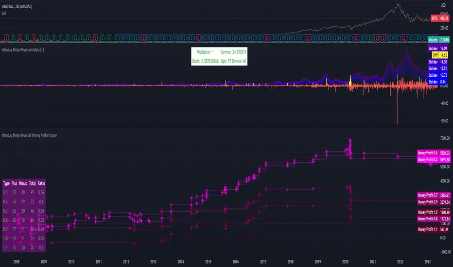
Intraday Mean Reversion Money Performance indicatorThe diagram shows Money Performance when buying stocks for 10 000 at every buy signal from the Intraday Mean Reversion indicator.
The indicator is best used in combination with Intraday Mean Reversion Main Indicator
The rules for trading are: Buy on Open price if the Intraday Mean Reversion Main indicator gives a buy signal. Sell on the daily close price.
According to my knowledge it is not possible to create a PineScript strategy based on these rules, because the indicator is used on Day to Day graph. Therefore this indicator can be used to analyze Money performance of this strategy.
The lines show the performance of the Intraday Mean Reversion Strategy, based on the different levels in the strategy (from 0.5 Standard deviation to 1.1 standard deviation)
Using this indicator it is possible to find stocks that often reverse towards mean after open.
Use this strategy on stocks with high positive performance. Do not use on stocks with negative performance.
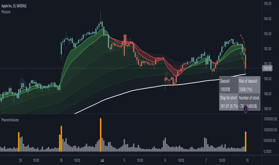
PhenomIt is a simple and effective tool for trading on moving averages.
The main advantage is that an ATR-based risk management system is included here. The system is based on the work of FullTimeTradingRu and the FBMA indicator
How to use the system:
1. I recommend using a daily timeframe.
2. Look for a rebound from the moving average, the most effective 20 Ema. For convenience, the colors of the bars are painted green in an uptrend.
3. Enter the transaction using hints. The recommended number of shares to buy is indicated in the table, taking into account your deposit and the risk per transaction from the deposit (by default 1%). Stop 1.5 ATR. Everything is the same for opening short positions.
4. I recommend entering the second trade only if the previous one passed 0.5 ATR, thereby confirming the trend and the fact that you correctly guessed the movement.
There are ATR settings in the script
Last bar show — How many bars to show
ATR lines ATR Step — For a more convenient view, ATR lines can be turned into a ladder.
Potential Gain/Loss IndicatorThis indicator calculates the gains and losses in percentage based on the highest high (ATH) and lowest low (ATL) of a given period. It takes the period as an input parameter and calculates the ATH and ATL within that period.
The indicator then calculates the potential gains in percentage if the price goes back to the ATH, as well as the potential losses in percentage if the price goes back to the ATL.
A filled area chart is plotted to show the difference between gains and losses (gains - losses) using a stepline, with green color when positive and red color when negative. The coefficient parameter allows for adjusting the scale of the gains and losses.
# Parameters
1. `period` (integer): The period used for calculating the highest high (ATH) and lowest low (ATL) within the given range. The default value is 50, and the user can select any value greater than or equal to 1.
2. `coef` (float): A coefficient to adjust the scale of the gains and losses. The default value is 0.5, and the user can select any value greater than or equal to 0.1.

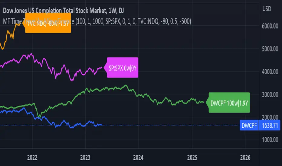
MF Time Travel (Delay or Forward Charts) by MigueFinanceThis indicator allows you to "Time Travel" aka. delay or advance (or forward) the on-screen chart/indicator as well as well as to do the same with other additional charts that can be configured in the settings.
This might be very useful when comparing with other (or the same) indicator in time, if you consider probably an incoming move based on another time performance.
About the Settings:
The moved in time charts can also be expanded or contracted, as well as they can be moved vertically (offset).
To Delay put positive values on the weeks settings, to Advance put Negative values on the same.
The Expansion or Contraction Factor is simply a multiplier of amplitude so you can multiply by number like 0.5, 2, etc
The Vertical Offset simply moves up and down the indicator.
The Labels will also tell you the number of weeks and years that were changed so as to have a reference, as well as the indicator being used.
Bearish Cypher Harmonic Patterns [theEccentricTrader]█ OVERVIEW
This indicator automatically draws bearish cypher harmonic patterns and price projections derived from the ranges that constitute the patterns.
█ CONCEPTS
Green and Red Candles
• A green candle is one that closes with a close price equal to or above the price it opened.
• A red candle is one that closes with a close price that is lower than the price it opened.
Swing Highs and Swing Lows
• A swing high is a green candle or series of consecutive green candles followed by a single red candle to complete the swing and form the peak.
• A swing low is a red candle or series of consecutive red candles followed by a single green candle to complete the swing and form the trough.
Peak and Trough Prices (Basic)
• The peak price of a complete swing high is the high price of either the red candle that completes the swing high or the high price of the preceding green candle, depending on which is higher.
• The trough price of a complete swing low is the low price of either the green candle that completes the swing low or the low price of the preceding red candle, depending on which is lower.
Historic Peaks and Troughs
The current, or most recent, peak and trough occurrences are referred to as occurrence zero. Previous peak and trough occurrences are referred to as historic and ordered numerically from right to left, with the most recent historic peak and trough occurrences being occurrence one.
Range
The range is simply the difference between the current peak and current trough prices, generally expressed in terms of points or pips.
Support and Resistance
• Support refers to a price level where the demand for an asset is strong enough to prevent the price from falling further.
• Resistance refers to a price level where the supply of an asset is strong enough to prevent the price from rising further.
Support and resistance levels are important because they can help traders identify where the price of an asset might pause or reverse its direction, offering potential entry and exit points. For example, a trader might look to buy an asset when it approaches a support level , with the expectation that the price will bounce back up. Alternatively, a trader might look to sell an asset when it approaches a resistance level , with the expectation that the price will drop back down.
It's important to note that support and resistance levels are not always relevant, and the price of an asset can also break through these levels and continue moving in the same direction.
Upper Trends
• A return line uptrend is formed when the current peak price is higher than the preceding peak price.
• A downtrend is formed when the current peak price is lower than the preceding peak price.
• A double-top is formed when the current peak price is equal to the preceding peak price.
Lower Trends
• An uptrend is formed when the current trough price is higher than the preceding trough price.
• A return line downtrend is formed when the current trough price is lower than the preceding trough price.
• A double-bottom is formed when the current trough price is equal to the preceding trough price.
Wave Cycles
A wave cycle is here defined as a complete two-part move between a swing high and a swing low, or a swing low and a swing high. The first swing high or swing low will set the course for the sequence of wave cycles that follow; for example a chart that begins with a swing low will form its first complete wave cycle upon the formation of the first complete swing high and vice versa.
Figure 1.
Fibonacci Retracement and Extension Ratios
The Fibonacci sequence is a series of numbers in which each number is the sum of the two preceding numbers, starting with 0 and 1. For example 0 + 1 = 1, 1 + 1 = 2, 1 + 2 = 3, and so on. Ultimately, we could go on forever but the first few numbers in the sequence are as follows: 0 , 1, 1, 2, 3, 5, 8, 13, 21, 34, 55, 89, 144.
The extension ratios are calculated by dividing each number in the sequence by the number preceding it. For example 0/1 = 0, 1/1 = 1, 2/1 = 2, 3/2 = 1.5, 5/3 = 1.6666..., 8/5 = 1.6, 13/8 = 1.625, 21/13 = 1.6153..., 34/21 = 1.6190..., 55/34 = 1.6176..., 89/55 = 1.6181..., 144/89 = 1.6179..., and so on. The retracement ratios are calculated by inverting this process and dividing each number in the sequence by the number proceeding it. For example 0/1 = 0, 1/1 = 1, 1/2 = 0.5, 2/3 = 0.666..., 3/5 = 0.6, 5/8 = 0.625, 8/13 = 0.6153..., 13/21 = 0.6190..., 21/34 = 0.6176..., 34/55 = 0.6181..., 55/89 = 0.6179..., 89/144 = 0.6180..., and so on.
1.618 is considered to be the 'golden ratio', found in many natural phenomena such as the growth of seashells and the branching of trees. Some now speculate the universe oscillates at a frequency of 0,618 Hz, which could help to explain such phenomena, but this theory has yet to be proven.
Traders and analysts use Fibonacci retracement and extension indicators, consisting of horizontal lines representing different Fibonacci ratios, for identifying potential levels of support and resistance. Fibonacci ranges are typically drawn from left to right, with retracement levels representing ratios inside of the current range and extension levels representing ratios extended outside of the current range. If the current wave cycle ends on a swing low, the Fibonacci range is drawn from peak to trough. If the current wave cycle ends on a swing high the Fibonacci range is drawn from trough to peak.
Harmonic Patterns
The concept of harmonic patterns in trading was first introduced by H.M. Gartley in his book "Profits in the Stock Market", published in 1935. Gartley observed that markets have a tendency to move in repetitive patterns, and he identified several specific patterns that he believed could be used to predict future price movements.
Since then, many other traders and analysts have built upon Gartley's work and developed their own variations of harmonic patterns. One such contributor is Larry Pesavento, who developed his own methods for measuring harmonic patterns using Fibonacci ratios. Pesavento has written several books on the subject of harmonic patterns and Fibonacci ratios in trading. Another notable contributor to harmonic patterns is Scott Carney, who developed his own approach to harmonic trading in the late 1990s and also popularised the use of Fibonacci ratios to measure harmonic patterns. Carney expanded on Gartley's work and also introduced several new harmonic patterns, such as the Shark pattern and the 5-0 pattern.
The bullish and bearish Gartley patterns are the oldest recognized harmonic patterns in trading and all the other harmonic patterns are ultimately modifications of the original Gartley patterns. Gartley patterns are fundamentally composed of 5 points, or 4 waves.
Bullish and Bearish Cypher Patterns
• Bullish cypher patterns are fundamentally composed of three troughs and two peaks, with the second peak being higher than the first peak and the second trough being higher than the first trough. The third trough must be lower than the second trough but higher than the first.
• Bearish cypher patterns are fundamentally composed of three peaks and two troughs, with the second trough being lower than the first trough and the second peak being lower than the first peak. The third peak must be higher than the second peak but lower than the first.
The most commonly recognised ratio measures used by traders today are as follows:
• Wave 1 of the pattern, referred to as XA, has no specific ratio requirements.
• Wave 2 of the pattern, referred to as AB, should retrace to at least 38.2%, but no further than 61.8% of the range set by wave 1.
• Wave 3 of the pattern, referred to as BC, should extend to at least 113%, but no further than 141.4% of the range set by wave 2.
• Wave 4 of the pattern, referred to as CD, should extend to at least 127.2%, but no further than 200% of the range set by wave 3.
• The last measure, that of wave 4 as a ratio of the range set between points X and C, referred to as XC, should retrace to 78.6%.
Measurement Tolerances
In general, tolerance in measurements refers to the allowable variation or deviation from a specific value or dimension. It is the range within which a particular measurement is considered to be acceptable or accurate. In this script I have applied this concept to the measurement of harmonic pattern ratios to increase to the frequency of pattern occurrences.
For example, the AB measurement of Gartley patterns is generally set at around 61.8%, but with such specificity in the measuring requirements the patterns are very rare. We can increase the frequency of pattern occurrences by setting a tolerance. A tolerance of 10% to both downside and upside, which is the default setting for all tolerances, means we would have a tolerable measurement range between 51.8-71.8%, thus increasing the frequency of occurrence.
█ FEATURES
Inputs
• AB Lower Tolerance
• AB Upper Tolerance
• BC Lower Tolerance
• BC Upper Tolerance
• CD Lower Tolerance
• CD Upper Tolerance
• XC Lower Tolerance
• XC Upper Tolerance
• Pattern Color
• Label Color
• Show Projections
• Extend Current Projection Lines
Alerts
Users can set alerts for when the patterns occur.
█ LIMITATIONS
All green and red candle calculations are based on differences between open and close prices, as such I have made no attempt to account for green candles that gap lower and close below the close price of the preceding candle, or red candles that gap higher and close above the close price of the preceding candle. This may cause some unexpected behaviour on some markets and timeframes. I can only recommend using 24-hour markets, if and where possible, as there are far fewer gaps and, generally, more data to work with.
█ NOTES
The cypher pattern was initially discovered by Darren Oglesbee, but I was unable to find any direct sources to his work on harmonic patterns. And although there seems to be some contention over whether or not there should be a ratio requirement for the CD wave, I decided to include it nonetheless.
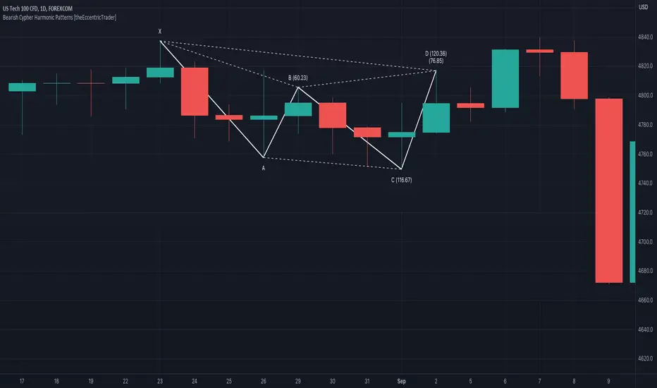
Bullish Cypher Harmonic Patterns [theEccentricTrader]█ OVERVIEW
This indicator automatically draws bullish cypher harmonic patterns and price projections derived from the ranges that constitute the patterns.
█ CONCEPTS
Green and Red Candles
• A green candle is one that closes with a close price equal to or above the price it opened.
• A red candle is one that closes with a close price that is lower than the price it opened.
Swing Highs and Swing Lows
• A swing high is a green candle or series of consecutive green candles followed by a single red candle to complete the swing and form the peak.
• A swing low is a red candle or series of consecutive red candles followed by a single green candle to complete the swing and form the trough.
Peak and Trough Prices (Basic)
• The peak price of a complete swing high is the high price of either the red candle that completes the swing high or the high price of the preceding green candle, depending on which is higher.
• The trough price of a complete swing low is the low price of either the green candle that completes the swing low or the low price of the preceding red candle, depending on which is lower.
Historic Peaks and Troughs
The current, or most recent, peak and trough occurrences are referred to as occurrence zero. Previous peak and trough occurrences are referred to as historic and ordered numerically from right to left, with the most recent historic peak and trough occurrences being occurrence one.
Range
The range is simply the difference between the current peak and current trough prices, generally expressed in terms of points or pips.
Support and Resistance
• Support refers to a price level where the demand for an asset is strong enough to prevent the price from falling further.
• Resistance refers to a price level where the supply of an asset is strong enough to prevent the price from rising further.
Support and resistance levels are important because they can help traders identify where the price of an asset might pause or reverse its direction, offering potential entry and exit points. For example, a trader might look to buy an asset when it approaches a support level , with the expectation that the price will bounce back up. Alternatively, a trader might look to sell an asset when it approaches a resistance level , with the expectation that the price will drop back down.
It's important to note that support and resistance levels are not always relevant, and the price of an asset can also break through these levels and continue moving in the same direction.
Upper Trends
• A return line uptrend is formed when the current peak price is higher than the preceding peak price.
• A downtrend is formed when the current peak price is lower than the preceding peak price.
• A double-top is formed when the current peak price is equal to the preceding peak price.
Lower Trends
• An uptrend is formed when the current trough price is higher than the preceding trough price.
• A return line downtrend is formed when the current trough price is lower than the preceding trough price.
• A double-bottom is formed when the current trough price is equal to the preceding trough price.
Wave Cycles
A wave cycle is here defined as a complete two-part move between a swing high and a swing low, or a swing low and a swing high. The first swing high or swing low will set the course for the sequence of wave cycles that follow; for example a chart that begins with a swing low will form its first complete wave cycle upon the formation of the first complete swing high and vice versa.
Figure 1.
Fibonacci Retracement and Extension Ratios
The Fibonacci sequence is a series of numbers in which each number is the sum of the two preceding numbers, starting with 0 and 1. For example 0 + 1 = 1, 1 + 1 = 2, 1 + 2 = 3, and so on. Ultimately, we could go on forever but the first few numbers in the sequence are as follows: 0 , 1, 1, 2, 3, 5, 8, 13, 21, 34, 55, 89, 144.
The extension ratios are calculated by dividing each number in the sequence by the number preceding it. For example 0/1 = 0, 1/1 = 1, 2/1 = 2, 3/2 = 1.5, 5/3 = 1.6666..., 8/5 = 1.6, 13/8 = 1.625, 21/13 = 1.6153..., 34/21 = 1.6190..., 55/34 = 1.6176..., 89/55 = 1.6181..., 144/89 = 1.6179..., and so on. The retracement ratios are calculated by inverting this process and dividing each number in the sequence by the number proceeding it. For example 0/1 = 0, 1/1 = 1, 1/2 = 0.5, 2/3 = 0.666..., 3/5 = 0.6, 5/8 = 0.625, 8/13 = 0.6153..., 13/21 = 0.6190..., 21/34 = 0.6176..., 34/55 = 0.6181..., 55/89 = 0.6179..., 89/144 = 0.6180..., and so on.
1.618 is considered to be the 'golden ratio', found in many natural phenomena such as the growth of seashells and the branching of trees. Some now speculate the universe oscillates at a frequency of 0,618 Hz, which could help to explain such phenomena, but this theory has yet to be proven.
Traders and analysts use Fibonacci retracement and extension indicators, consisting of horizontal lines representing different Fibonacci ratios, for identifying potential levels of support and resistance. Fibonacci ranges are typically drawn from left to right, with retracement levels representing ratios inside of the current range and extension levels representing ratios extended outside of the current range. If the current wave cycle ends on a swing low, the Fibonacci range is drawn from peak to trough. If the current wave cycle ends on a swing high the Fibonacci range is drawn from trough to peak.
Harmonic Patterns
The concept of harmonic patterns in trading was first introduced by H.M. Gartley in his book "Profits in the Stock Market", published in 1935. Gartley observed that markets have a tendency to move in repetitive patterns, and he identified several specific patterns that he believed could be used to predict future price movements.
Since then, many other traders and analysts have built upon Gartley's work and developed their own variations of harmonic patterns. One such contributor is Larry Pesavento, who developed his own methods for measuring harmonic patterns using Fibonacci ratios. Pesavento has written several books on the subject of harmonic patterns and Fibonacci ratios in trading. Another notable contributor to harmonic patterns is Scott Carney, who developed his own approach to harmonic trading in the late 1990s and also popularised the use of Fibonacci ratios to measure harmonic patterns. Carney expanded on Gartley's work and also introduced several new harmonic patterns, such as the Shark pattern and the 5-0 pattern.
The bullish and bearish Gartley patterns are the oldest recognized harmonic patterns in trading and all the other harmonic patterns are ultimately modifications of the original Gartley patterns. Gartley patterns are fundamentally composed of 5 points, or 4 waves.
Bullish and Bearish Cypher Patterns
• Bullish cypher patterns are fundamentally composed of three troughs and two peaks, with the second peak being higher than the first peak and the second trough being higher than the first trough. The third trough must be lower than the second trough but higher than the first.
• Bearish cypher patterns are fundamentally composed of three peaks and two troughs, with the second trough being lower than the first trough and the second peak being lower than the first peak. The third peak must be higher than the second peak but lower than the first.
The most commonly recognised ratio measures used by traders today are as follows:
• Wave 1 of the pattern, referred to as XA, has no specific ratio requirements.
• Wave 2 of the pattern, referred to as AB, should retrace to at least 38.2%, but no further than 61.8% of the range set by wave 1.
• Wave 3 of the pattern, referred to as BC, should extend to at least 113%, but no further than 141.4% of the range set by wave 2.
• Wave 4 of the pattern, referred to as CD, should extend to at least 127.2%, but no further than 200% of the range set by wave 3.
• The last measure, that of wave 4 as a ratio of the range set between points X and C, referred to as XC, should retrace to 78.6%.
Measurement Tolerances
In general, tolerance in measurements refers to the allowable variation or deviation from a specific value or dimension. It is the range within which a particular measurement is considered to be acceptable or accurate. In this script I have applied this concept to the measurement of harmonic pattern ratios to increase to the frequency of pattern occurrences.
For example, the AB measurement of Gartley patterns is generally set at around 61.8%, but with such specificity in the measuring requirements the patterns are very rare. We can increase the frequency of pattern occurrences by setting a tolerance. A tolerance of 10% to both downside and upside, which is the default setting for all tolerances, means we would have a tolerable measurement range between 51.8-71.8%, thus increasing the frequency of occurrence.
█ FEATURES
Inputs
• AB Lower Tolerance
• AB Upper Tolerance
• BC Lower Tolerance
• BC Upper Tolerance
• CD Lower Tolerance
• CD Upper Tolerance
• XC Lower Tolerance
• XC Upper Tolerance
• Pattern Color
• Label Color
• Show Projections
• Extend Current Projection Lines
Alerts
Users can set alerts for when the patterns occur.
█ LIMITATIONS
All green and red candle calculations are based on differences between open and close prices, as such I have made no attempt to account for green candles that gap lower and close below the close price of the preceding candle, or red candles that gap higher and close above the close price of the preceding candle. This may cause some unexpected behaviour on some markets and timeframes. I can only recommend using 24-hour markets, if and where possible, as there are far fewer gaps and, generally, more data to work with.
█ NOTES
The cypher pattern was initially discovered by Darren Oglesbee, but I was unable to find any direct sources to his work on harmonic patterns. And although there seems to be some contention over whether or not there should be a ratio requirement for the CD wave, I decided to include it nonetheless.
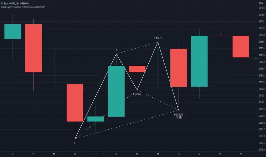
Bearish Deep Crab Harmonic Patterns [theEccentricTrader]█ OVERVIEW
This indicator automatically draws bearish deep crab harmonic patterns and price projections derived from the ranges that constitute the patterns.
█ CONCEPTS
Green and Red Candles
• A green candle is one that closes with a close price equal to or above the price it opened.
• A red candle is one that closes with a close price that is lower than the price it opened.
Swing Highs and Swing Lows
• A swing high is a green candle or series of consecutive green candles followed by a single red candle to complete the swing and form the peak.
• A swing low is a red candle or series of consecutive red candles followed by a single green candle to complete the swing and form the trough.
Peak and Trough Prices (Basic)
• The peak price of a complete swing high is the high price of either the red candle that completes the swing high or the high price of the preceding green candle, depending on which is higher.
• The trough price of a complete swing low is the low price of either the green candle that completes the swing low or the low price of the preceding red candle, depending on which is lower.
Historic Peaks and Troughs
The current, or most recent, peak and trough occurrences are referred to as occurrence zero. Previous peak and trough occurrences are referred to as historic and ordered numerically from right to left, with the most recent historic peak and trough occurrences being occurrence one.
Range
The range is simply the difference between the current peak and current trough prices, generally expressed in terms of points or pips.
Support and Resistance
• Support refers to a price level where the demand for an asset is strong enough to prevent the price from falling further.
• Resistance refers to a price level where the supply of an asset is strong enough to prevent the price from rising further.
Support and resistance levels are important because they can help traders identify where the price of an asset might pause or reverse its direction, offering potential entry and exit points. For example, a trader might look to buy an asset when it approaches a support level , with the expectation that the price will bounce back up. Alternatively, a trader might look to sell an asset when it approaches a resistance level , with the expectation that the price will drop back down.
It's important to note that support and resistance levels are not always relevant, and the price of an asset can also break through these levels and continue moving in the same direction.
Upper Trends
• A return line uptrend is formed when the current peak price is higher than the preceding peak price.
• A downtrend is formed when the current peak price is lower than the preceding peak price.
• A double-top is formed when the current peak price is equal to the preceding peak price.
Lower Trends
• An uptrend is formed when the current trough price is higher than the preceding trough price.
• A return line downtrend is formed when the current trough price is lower than the preceding trough price.
• A double-bottom is formed when the current trough price is equal to the preceding trough price.
Wave Cycles
A wave cycle is here defined as a complete two-part move between a swing high and a swing low, or a swing low and a swing high. The first swing high or swing low will set the course for the sequence of wave cycles that follow; for example a chart that begins with a swing low will form its first complete wave cycle upon the formation of the first complete swing high and vice versa.
Figure 1.
Fibonacci Retracement and Extension Ratios
The Fibonacci sequence is a series of numbers in which each number is the sum of the two preceding numbers, starting with 0 and 1. For example 0 + 1 = 1, 1 + 1 = 2, 1 + 2 = 3, and so on. Ultimately, we could go on forever but the first few numbers in the sequence are as follows: 0 , 1, 1, 2, 3, 5, 8, 13, 21, 34, 55, 89, 144.
The extension ratios are calculated by dividing each number in the sequence by the number preceding it. For example 0/1 = 0, 1/1 = 1, 2/1 = 2, 3/2 = 1.5, 5/3 = 1.6666..., 8/5 = 1.6, 13/8 = 1.625, 21/13 = 1.6153..., 34/21 = 1.6190..., 55/34 = 1.6176..., 89/55 = 1.6181..., 144/89 = 1.6179..., and so on. The retracement ratios are calculated by inverting this process and dividing each number in the sequence by the number proceeding it. For example 0/1 = 0, 1/1 = 1, 1/2 = 0.5, 2/3 = 0.666..., 3/5 = 0.6, 5/8 = 0.625, 8/13 = 0.6153..., 13/21 = 0.6190..., 21/34 = 0.6176..., 34/55 = 0.6181..., 55/89 = 0.6179..., 89/144 = 0.6180..., and so on.
1.618 is considered to be the 'golden ratio', found in many natural phenomena such as the growth of seashells and the branching of trees. Some now speculate the universe oscillates at a frequency of 0,618 Hz, which could help to explain such phenomena, but this theory has yet to be proven.
Traders and analysts use Fibonacci retracement and extension indicators, consisting of horizontal lines representing different Fibonacci ratios, for identifying potential levels of support and resistance. Fibonacci ranges are typically drawn from left to right, with retracement levels representing ratios inside of the current range and extension levels representing ratios extended outside of the current range. If the current wave cycle ends on a swing low, the Fibonacci range is drawn from peak to trough. If the current wave cycle ends on a swing high the Fibonacci range is drawn from trough to peak.
Harmonic Patterns
The concept of harmonic patterns in trading was first introduced by H.M. Gartley in his book "Profits in the Stock Market", published in 1935. Gartley observed that markets have a tendency to move in repetitive patterns, and he identified several specific patterns that he believed could be used to predict future price movements.
Since then, many other traders and analysts have built upon Gartley's work and developed their own variations of harmonic patterns. One such contributor is Larry Pesavento, who developed his own methods for measuring harmonic patterns using Fibonacci ratios. Pesavento has written several books on the subject of harmonic patterns and Fibonacci ratios in trading. Another notable contributor to harmonic patterns is Scott Carney, who developed his own approach to harmonic trading in the late 1990s and also popularised the use of Fibonacci ratios to measure harmonic patterns. Carney expanded on Gartley's work and also introduced several new harmonic patterns, such as the Shark pattern and the 5-0 pattern.
The bullish and bearish Gartley patterns are the oldest recognized harmonic patterns in trading and all the other harmonic patterns are ultimately modifications of the original Gartley patterns. Gartley patterns are fundamentally composed of 5 points, or 4 waves.
Bullish and Bearish Deep Crab Patterns
• Bullish deep crab patterns are fundamentally composed of three troughs and two peaks. The second peak being lower than the first peak. And the third trough being lower than both the first and second troughs, while the second trough is higher than the first.
• Bearish deep crab patterns are fundamentally composed of three peaks and two troughs. The second trough being higher than the first trough. And the third peak being higher than both the first and second peaks, while the second peak is lower than the first.
The ratio measurements recommended by Scott Carney, who originated the pattern, are as follows:
• Wave 1 of the pattern, generally referred to as XA, has no specific ratio requirements.
• Wave 2 of the pattern, generally referred to as AB, should retrace to 88.6% of the range set by wave 1.
• Wave 3 of the pattern, generally referred to as BC, should retrace by at least 38.2%, but no further than 88.6% of the range set by wave 2.
• Wave 4 of the pattern, generally referred to as CD, should extend to at least 200%, but no further than 361.8% of the range set by wave 3.
• The last measure, generally referred to as AD, is that of wave 4 as a ratio of the range set by wave 1, which should extend to 161.8%.
Measurement Tolerances
In general, tolerance in measurements refers to the allowable variation or deviation from a specific value or dimension. It is the range within which a particular measurement is considered to be acceptable or accurate. In this script I have applied this concept to the measurement of harmonic pattern ratios to increase to the frequency of pattern occurrences.
For example, the AB measurement of Gartley patterns is generally set at around 61.8%, but with such specificity in the measuring requirements the patterns are very rare. We can increase the frequency of pattern occurrences by setting a tolerance. A tolerance of 10% to both downside and upside, which is the default setting for all tolerances, means we would have a tolerable measurement range between 51.8-71.8%, thus increasing the frequency of occurrence.
█ FEATURES
Inputs
• AB Lower Tolerance
• AB Upper Tolerance
• BC Lower Tolerance
• BC Upper Tolerance
• CD Lower Tolerance
• CD Upper Tolerance
• AD Lower Tolerance
• AD Upper Tolerance
• Pattern Color
• Label Color
• Show Projections
• Extend Current Projection Lines
Alerts
Users can set alerts for when the patterns occur.
█ LIMITATIONS
All green and red candle calculations are based on differences between open and close prices, as such I have made no attempt to account for green candles that gap lower and close below the close price of the preceding candle, or red candles that gap higher and close above the close price of the preceding candle. This may cause some unexpected behaviour on some markets and timeframes. I can only recommend using 24-hour markets, if and where possible, as there are far fewer gaps and, generally, more data to work with.
█ NOTES
A link to Scott's harmonic patterns webpage for anyone who may be interested: harmonictrader.com/harmonic-patterns/

Bullish Deep Crab Harmonic Patterns [theEccentricTrader]█ OVERVIEW
This indicator automatically draws bullish deep crab harmonic patterns and price projections derived from the ranges that constitute the patterns.
█ CONCEPTS
Green and Red Candles
• A green candle is one that closes with a close price equal to or above the price it opened.
• A red candle is one that closes with a close price that is lower than the price it opened.
Swing Highs and Swing Lows
• A swing high is a green candle or series of consecutive green candles followed by a single red candle to complete the swing and form the peak.
• A swing low is a red candle or series of consecutive red candles followed by a single green candle to complete the swing and form the trough.
Peak and Trough Prices (Basic)
• The peak price of a complete swing high is the high price of either the red candle that completes the swing high or the high price of the preceding green candle, depending on which is higher.
• The trough price of a complete swing low is the low price of either the green candle that completes the swing low or the low price of the preceding red candle, depending on which is lower.
Historic Peaks and Troughs
The current, or most recent, peak and trough occurrences are referred to as occurrence zero. Previous peak and trough occurrences are referred to as historic and ordered numerically from right to left, with the most recent historic peak and trough occurrences being occurrence one.
Range
The range is simply the difference between the current peak and current trough prices, generally expressed in terms of points or pips.
Support and Resistance
• Support refers to a price level where the demand for an asset is strong enough to prevent the price from falling further.
• Resistance refers to a price level where the supply of an asset is strong enough to prevent the price from rising further.
Support and resistance levels are important because they can help traders identify where the price of an asset might pause or reverse its direction, offering potential entry and exit points. For example, a trader might look to buy an asset when it approaches a support level , with the expectation that the price will bounce back up. Alternatively, a trader might look to sell an asset when it approaches a resistance level , with the expectation that the price will drop back down.
It's important to note that support and resistance levels are not always relevant, and the price of an asset can also break through these levels and continue moving in the same direction.
Upper Trends
• A return line uptrend is formed when the current peak price is higher than the preceding peak price.
• A downtrend is formed when the current peak price is lower than the preceding peak price.
• A double-top is formed when the current peak price is equal to the preceding peak price.
Lower Trends
• An uptrend is formed when the current trough price is higher than the preceding trough price.
• A return line downtrend is formed when the current trough price is lower than the preceding trough price.
• A double-bottom is formed when the current trough price is equal to the preceding trough price.
Wave Cycles
A wave cycle is here defined as a complete two-part move between a swing high and a swing low, or a swing low and a swing high. The first swing high or swing low will set the course for the sequence of wave cycles that follow; for example a chart that begins with a swing low will form its first complete wave cycle upon the formation of the first complete swing high and vice versa.
Figure 1.
Fibonacci Retracement and Extension Ratios
The Fibonacci sequence is a series of numbers in which each number is the sum of the two preceding numbers, starting with 0 and 1. For example 0 + 1 = 1, 1 + 1 = 2, 1 + 2 = 3, and so on. Ultimately, we could go on forever but the first few numbers in the sequence are as follows: 0 , 1, 1, 2, 3, 5, 8, 13, 21, 34, 55, 89, 144.
The extension ratios are calculated by dividing each number in the sequence by the number preceding it. For example 0/1 = 0, 1/1 = 1, 2/1 = 2, 3/2 = 1.5, 5/3 = 1.6666..., 8/5 = 1.6, 13/8 = 1.625, 21/13 = 1.6153..., 34/21 = 1.6190..., 55/34 = 1.6176..., 89/55 = 1.6181..., 144/89 = 1.6179..., and so on. The retracement ratios are calculated by inverting this process and dividing each number in the sequence by the number proceeding it. For example 0/1 = 0, 1/1 = 1, 1/2 = 0.5, 2/3 = 0.666..., 3/5 = 0.6, 5/8 = 0.625, 8/13 = 0.6153..., 13/21 = 0.6190..., 21/34 = 0.6176..., 34/55 = 0.6181..., 55/89 = 0.6179..., 89/144 = 0.6180..., and so on.
1.618 is considered to be the 'golden ratio', found in many natural phenomena such as the growth of seashells and the branching of trees. Some now speculate the universe oscillates at a frequency of 0,618 Hz, which could help to explain such phenomena, but this theory has yet to be proven.
Traders and analysts use Fibonacci retracement and extension indicators, consisting of horizontal lines representing different Fibonacci ratios, for identifying potential levels of support and resistance. Fibonacci ranges are typically drawn from left to right, with retracement levels representing ratios inside of the current range and extension levels representing ratios extended outside of the current range. If the current wave cycle ends on a swing low, the Fibonacci range is drawn from peak to trough. If the current wave cycle ends on a swing high the Fibonacci range is drawn from trough to peak.
Harmonic Patterns
The concept of harmonic patterns in trading was first introduced by H.M. Gartley in his book "Profits in the Stock Market", published in 1935. Gartley observed that markets have a tendency to move in repetitive patterns, and he identified several specific patterns that he believed could be used to predict future price movements.
Since then, many other traders and analysts have built upon Gartley's work and developed their own variations of harmonic patterns. One such contributor is Larry Pesavento, who developed his own methods for measuring harmonic patterns using Fibonacci ratios. Pesavento has written several books on the subject of harmonic patterns and Fibonacci ratios in trading. Another notable contributor to harmonic patterns is Scott Carney, who developed his own approach to harmonic trading in the late 1990s and also popularised the use of Fibonacci ratios to measure harmonic patterns. Carney expanded on Gartley's work and also introduced several new harmonic patterns, such as the Shark pattern and the 5-0 pattern.
The bullish and bearish Gartley patterns are the oldest recognized harmonic patterns in trading and all the other harmonic patterns are ultimately modifications of the original Gartley patterns. Gartley patterns are fundamentally composed of 5 points, or 4 waves.
Bullish and Bearish Deep Crab Patterns
• Bullish deep crab patterns are fundamentally composed of three troughs and two peaks. The second peak being lower than the first peak. And the third trough being lower than both the first and second troughs, while the second trough is higher than the first.
• Bearish deep crab patterns are fundamentally composed of three peaks and two troughs. The second trough being higher than the first trough. And the third peak being higher than both the first and second peaks, while the second peak is lower than the first.
The ratio measurements recommended by Scott Carney, who originated the pattern, are as follows:
• Wave 1 of the pattern, generally referred to as XA, has no specific ratio requirements.
• Wave 2 of the pattern, generally referred to as AB, should retrace to 88.6% of the range set by wave 1.
• Wave 3 of the pattern, generally referred to as BC, should retrace by at least 38.2%, but no further than 88.6% of the range set by wave 2.
• Wave 4 of the pattern, generally referred to as CD, should extend to at least 200%, but no further than 361.8% of the range set by wave 3.
• The last measure, generally referred to as AD, is that of wave 4 as a ratio of the range set by wave 1, which should extend to 161.8%.
Measurement Tolerances
In general, tolerance in measurements refers to the allowable variation or deviation from a specific value or dimension. It is the range within which a particular measurement is considered to be acceptable or accurate. In this script I have applied this concept to the measurement of harmonic pattern ratios to increase to the frequency of pattern occurrences.
For example, the AB measurement of Gartley patterns is generally set at around 61.8%, but with such specificity in the measuring requirements the patterns are very rare. We can increase the frequency of pattern occurrences by setting a tolerance. A tolerance of 10% to both downside and upside, which is the default setting for all tolerances, means we would have a tolerable measurement range between 51.8-71.8%, thus increasing the frequency of occurrence.
█ FEATURES
Inputs
• AB Lower Tolerance
• AB Upper Tolerance
• BC Lower Tolerance
• BC Upper Tolerance
• CD Lower Tolerance
• CD Upper Tolerance
• AD Lower Tolerance
• AD Upper Tolerance
• Pattern Color
• Label Color
• Show Projections
• Extend Current Projection Lines
Alerts
Users can set alerts for when the patterns occur.
█ LIMITATIONS
All green and red candle calculations are based on differences between open and close prices, as such I have made no attempt to account for green candles that gap lower and close below the close price of the preceding candle, or red candles that gap higher and close above the close price of the preceding candle. This may cause some unexpected behaviour on some markets and timeframes. I can only recommend using 24-hour markets, if and where possible, as there are far fewer gaps and, generally, more data to work with.
█ NOTES
A link to Scott's harmonic patterns webpage for anyone who may be interested: harmonictrader.com/harmonic-patterns/
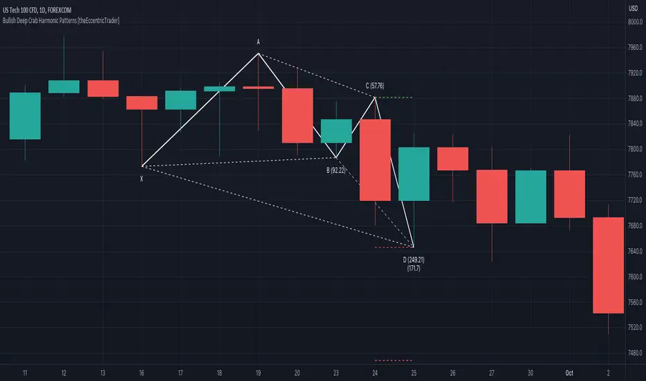
Bearish Alternate Bat Harmonic Patterns [theEccentricTrader]█ OVERVIEW
This indicator automatically draws bearish alternate bat harmonic patterns and price projections derived from the ranges that constitute the patterns.
█ CONCEPTS
Green and Red Candles
• A green candle is one that closes with a close price equal to or above the price it opened.
• A red candle is one that closes with a close price that is lower than the price it opened.
Swing Highs and Swing Lows
• A swing high is a green candle or series of consecutive green candles followed by a single red candle to complete the swing and form the peak.
• A swing low is a red candle or series of consecutive red candles followed by a single green candle to complete the swing and form the trough.
Peak and Trough Prices (Basic)
• The peak price of a complete swing high is the high price of either the red candle that completes the swing high or the high price of the preceding green candle, depending on which is higher.
• The trough price of a complete swing low is the low price of either the green candle that completes the swing low or the low price of the preceding red candle, depending on which is lower.
Historic Peaks and Troughs
The current, or most recent, peak and trough occurrences are referred to as occurrence zero. Previous peak and trough occurrences are referred to as historic and ordered numerically from right to left, with the most recent historic peak and trough occurrences being occurrence one.
Range
The range is simply the difference between the current peak and current trough prices, generally expressed in terms of points or pips.
Support and Resistance
• Support refers to a price level where the demand for an asset is strong enough to prevent the price from falling further.
• Resistance refers to a price level where the supply of an asset is strong enough to prevent the price from rising further.
Support and resistance levels are important because they can help traders identify where the price of an asset might pause or reverse its direction, offering potential entry and exit points. For example, a trader might look to buy an asset when it approaches a support level , with the expectation that the price will bounce back up. Alternatively, a trader might look to sell an asset when it approaches a resistance level , with the expectation that the price will drop back down.
It's important to note that support and resistance levels are not always relevant, and the price of an asset can also break through these levels and continue moving in the same direction.
Upper Trends
• A return line uptrend is formed when the current peak price is higher than the preceding peak price.
• A downtrend is formed when the current peak price is lower than the preceding peak price.
• A double-top is formed when the current peak price is equal to the preceding peak price.
Lower Trends
• An uptrend is formed when the current trough price is higher than the preceding trough price.
• A return line downtrend is formed when the current trough price is lower than the preceding trough price.
• A double-bottom is formed when the current trough price is equal to the preceding trough price.
Wave Cycles
A wave cycle is here defined as a complete two-part move between a swing high and a swing low, or a swing low and a swing high. The first swing high or swing low will set the course for the sequence of wave cycles that follow; for example a chart that begins with a swing low will form its first complete wave cycle upon the formation of the first complete swing high and vice versa.
Figure 1.
Fibonacci Retracement and Extension Ratios
The Fibonacci sequence is a series of numbers in which each number is the sum of the two preceding numbers, starting with 0 and 1. For example 0 + 1 = 1, 1 + 1 = 2, 1 + 2 = 3, and so on. Ultimately, we could go on forever but the first few numbers in the sequence are as follows: 0 , 1, 1, 2, 3, 5, 8, 13, 21, 34, 55, 89, 144.
The extension ratios are calculated by dividing each number in the sequence by the number preceding it. For example 0/1 = 0, 1/1 = 1, 2/1 = 2, 3/2 = 1.5, 5/3 = 1.6666..., 8/5 = 1.6, 13/8 = 1.625, 21/13 = 1.6153..., 34/21 = 1.6190..., 55/34 = 1.6176..., 89/55 = 1.6181..., 144/89 = 1.6179..., and so on. The retracement ratios are calculated by inverting this process and dividing each number in the sequence by the number proceeding it. For example 0/1 = 0, 1/1 = 1, 1/2 = 0.5, 2/3 = 0.666..., 3/5 = 0.6, 5/8 = 0.625, 8/13 = 0.6153..., 13/21 = 0.6190..., 21/34 = 0.6176..., 34/55 = 0.6181..., 55/89 = 0.6179..., 89/144 = 0.6180..., and so on.
1.618 is considered to be the 'golden ratio', found in many natural phenomena such as the growth of seashells and the branching of trees. Some now speculate the universe oscillates at a frequency of 0,618 Hz, which could help to explain such phenomena, but this theory has yet to be proven.
Traders and analysts use Fibonacci retracement and extension indicators, consisting of horizontal lines representing different Fibonacci ratios, for identifying potential levels of support and resistance. Fibonacci ranges are typically drawn from left to right, with retracement levels representing ratios inside of the current range and extension levels representing ratios extended outside of the current range. If the current wave cycle ends on a swing low, the Fibonacci range is drawn from peak to trough. If the current wave cycle ends on a swing high the Fibonacci range is drawn from trough to peak.
Harmonic Patterns
The concept of harmonic patterns in trading was first introduced by H.M. Gartley in his book "Profits in the Stock Market", published in 1935. Gartley observed that markets have a tendency to move in repetitive patterns, and he identified several specific patterns that he believed could be used to predict future price movements.
Since then, many other traders and analysts have built upon Gartley's work and developed their own variations of harmonic patterns. One such contributor is Larry Pesavento, who developed his own methods for measuring harmonic patterns using Fibonacci ratios. Pesavento has written several books on the subject of harmonic patterns and Fibonacci ratios in trading. Another notable contributor to harmonic patterns is Scott Carney, who developed his own approach to harmonic trading in the late 1990s and also popularised the use of Fibonacci ratios to measure harmonic patterns. Carney expanded on Gartley's work and also introduced several new harmonic patterns, such as the Shark pattern and the 5-0 pattern.
The bullish and bearish Gartley patterns are the oldest recognized harmonic patterns in trading and all the other harmonic patterns are ultimately modifications of the original Gartley patterns. Gartley patterns are fundamentally composed of 5 points, or 4 waves.
Bullish and Bearish Alternate Bat Patterns
• Bullish alternate bat patterns are fundamentally composed of three troughs and two peaks. The second peak being lower than the first peak and the second trough being higher than the first, with the third trough being lower than both the first and second troughs.
• Bearish alternate bat patterns are fundamentally composed of three peaks and two troughs. The second trough being higher than the first trough and the second peak being lower than the first, with the third peak being higher than both the first and second peaks.
The ratio measurements recommended by Scott Carney, who originated the pattern, are as follows:
• Wave 1 of the pattern, generally referred to as XA, has no specific ratio requirements.
• Wave 2 of the pattern, generally referred to as AB, should retrace to 38.2% of the range set by wave 1.
• Wave 3 of the pattern, generally referred to as BC, should retrace by at least 38.2%, but no further than 88.6% of the range set by wave 2.
• Wave 4 of the pattern, generally referred to as CD, should extend to at least 200%, but no further than 361.8% of the range set by wave 3.
• The last measure, generally referred to as AD, is that of wave 4 as a ratio of the range set by wave 1, which should extend to 113%.
Measurement Tolerances
In general, tolerance in measurements refers to the allowable variation or deviation from a specific value or dimension. It is the range within which a particular measurement is considered to be acceptable or accurate. In this script I have applied this concept to the measurement of harmonic pattern ratios to increase to the frequency of pattern occurrences.
For example, the AB measurement of Gartley patterns is generally set at around 61.8%, but with such specificity in the measuring requirements the patterns are very rare. We can increase the frequency of pattern occurrences by setting a tolerance. A tolerance of 10% to both downside and upside, which is the default setting for all tolerances, means we would have a tolerable measurement range between 51.8-71.8%, thus increasing the frequency of occurrence.
█ FEATURES
Inputs
• AB Lower Tolerance
• AB Upper Tolerance
• BC Lower Tolerance
• BC Upper Tolerance
• CD Lower Tolerance
• CD Upper Tolerance
• AD Lower Tolerance
• AD Upper Tolerance
• Pattern Color
• Label Color
• Show Projections
• Extend Current Projection Lines
Alerts
Users can set alerts for when the patterns occur.
█ LIMITATIONS
All green and red candle calculations are based on differences between open and close prices, as such I have made no attempt to account for green candles that gap lower and close below the close price of the preceding candle, or red candles that gap higher and close above the close price of the preceding candle. This may cause some unexpected behaviour on some markets and timeframes. I can only recommend using 24-hour markets, if and where possible, as there are far fewer gaps and, generally, more data to work with.
█ NOTES
A link to Scott's harmonic patterns webpage for anyone who may be interested: harmonictrader.com/harmonic-patterns/
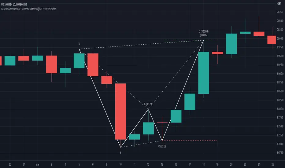
Bullish Alternate Bat Harmonic Patterns [theEccentricTrader]█ OVERVIEW
This indicator automatically draws bullish alternate bat harmonic patterns and price projections derived from the ranges that constitute the patterns.
█ CONCEPTS
Green and Red Candles
• A green candle is one that closes with a close price equal to or above the price it opened.
• A red candle is one that closes with a close price that is lower than the price it opened.
Swing Highs and Swing Lows
• A swing high is a green candle or series of consecutive green candles followed by a single red candle to complete the swing and form the peak.
• A swing low is a red candle or series of consecutive red candles followed by a single green candle to complete the swing and form the trough.
Peak and Trough Prices (Basic)
• The peak price of a complete swing high is the high price of either the red candle that completes the swing high or the high price of the preceding green candle, depending on which is higher.
• The trough price of a complete swing low is the low price of either the green candle that completes the swing low or the low price of the preceding red candle, depending on which is lower.
Historic Peaks and Troughs
The current, or most recent, peak and trough occurrences are referred to as occurrence zero. Previous peak and trough occurrences are referred to as historic and ordered numerically from right to left, with the most recent historic peak and trough occurrences being occurrence one.
Range
The range is simply the difference between the current peak and current trough prices, generally expressed in terms of points or pips.
Support and Resistance
• Support refers to a price level where the demand for an asset is strong enough to prevent the price from falling further.
• Resistance refers to a price level where the supply of an asset is strong enough to prevent the price from rising further.
Support and resistance levels are important because they can help traders identify where the price of an asset might pause or reverse its direction, offering potential entry and exit points. For example, a trader might look to buy an asset when it approaches a support level , with the expectation that the price will bounce back up. Alternatively, a trader might look to sell an asset when it approaches a resistance level , with the expectation that the price will drop back down.
It's important to note that support and resistance levels are not always relevant, and the price of an asset can also break through these levels and continue moving in the same direction.
Upper Trends
• A return line uptrend is formed when the current peak price is higher than the preceding peak price.
• A downtrend is formed when the current peak price is lower than the preceding peak price.
• A double-top is formed when the current peak price is equal to the preceding peak price.
Lower Trends
• An uptrend is formed when the current trough price is higher than the preceding trough price.
• A return line downtrend is formed when the current trough price is lower than the preceding trough price.
• A double-bottom is formed when the current trough price is equal to the preceding trough price.
Wave Cycles
A wave cycle is here defined as a complete two-part move between a swing high and a swing low, or a swing low and a swing high. The first swing high or swing low will set the course for the sequence of wave cycles that follow; for example a chart that begins with a swing low will form its first complete wave cycle upon the formation of the first complete swing high and vice versa.
Figure 1.
Fibonacci Retracement and Extension Ratios
The Fibonacci sequence is a series of numbers in which each number is the sum of the two preceding numbers, starting with 0 and 1. For example 0 + 1 = 1, 1 + 1 = 2, 1 + 2 = 3, and so on. Ultimately, we could go on forever but the first few numbers in the sequence are as follows: 0 , 1, 1, 2, 3, 5, 8, 13, 21, 34, 55, 89, 144.
The extension ratios are calculated by dividing each number in the sequence by the number preceding it. For example 0/1 = 0, 1/1 = 1, 2/1 = 2, 3/2 = 1.5, 5/3 = 1.6666..., 8/5 = 1.6, 13/8 = 1.625, 21/13 = 1.6153..., 34/21 = 1.6190..., 55/34 = 1.6176..., 89/55 = 1.6181..., 144/89 = 1.6179..., and so on. The retracement ratios are calculated by inverting this process and dividing each number in the sequence by the number proceeding it. For example 0/1 = 0, 1/1 = 1, 1/2 = 0.5, 2/3 = 0.666..., 3/5 = 0.6, 5/8 = 0.625, 8/13 = 0.6153..., 13/21 = 0.6190..., 21/34 = 0.6176..., 34/55 = 0.6181..., 55/89 = 0.6179..., 89/144 = 0.6180..., and so on.
1.618 is considered to be the 'golden ratio', found in many natural phenomena such as the growth of seashells and the branching of trees. Some now speculate the universe oscillates at a frequency of 0,618 Hz, which could help to explain such phenomena, but this theory has yet to be proven.
Traders and analysts use Fibonacci retracement and extension indicators, consisting of horizontal lines representing different Fibonacci ratios, for identifying potential levels of support and resistance. Fibonacci ranges are typically drawn from left to right, with retracement levels representing ratios inside of the current range and extension levels representing ratios extended outside of the current range. If the current wave cycle ends on a swing low, the Fibonacci range is drawn from peak to trough. If the current wave cycle ends on a swing high the Fibonacci range is drawn from trough to peak.
Harmonic Patterns
The concept of harmonic patterns in trading was first introduced by H.M. Gartley in his book "Profits in the Stock Market", published in 1935. Gartley observed that markets have a tendency to move in repetitive patterns, and he identified several specific patterns that he believed could be used to predict future price movements.
Since then, many other traders and analysts have built upon Gartley's work and developed their own variations of harmonic patterns. One such contributor is Larry Pesavento, who developed his own methods for measuring harmonic patterns using Fibonacci ratios. Pesavento has written several books on the subject of harmonic patterns and Fibonacci ratios in trading. Another notable contributor to harmonic patterns is Scott Carney, who developed his own approach to harmonic trading in the late 1990s and also popularised the use of Fibonacci ratios to measure harmonic patterns. Carney expanded on Gartley's work and also introduced several new harmonic patterns, such as the Shark pattern and the 5-0 pattern.
The bullish and bearish Gartley patterns are the oldest recognized harmonic patterns in trading and all the other harmonic patterns are ultimately modifications of the original Gartley patterns. Gartley patterns are fundamentally composed of 5 points, or 4 waves.
Bullish and Bearish Alternate Bat Patterns
• Bullish alternate bat patterns are fundamentally composed of three troughs and two peaks. The second peak being lower than the first peak and the second trough being higher than the first, with the third trough being lower than both the first and second troughs.
• Bearish alternate bat patterns are fundamentally composed of three peaks and two troughs. The second trough being higher than the first trough and the second peak being lower than the first, with the third peak being higher than both the first and second peaks.
The ratio measurements recommended by Scott Carney, who originated the pattern, are as follows:
• Wave 1 of the pattern, generally referred to as XA, has no specific ratio requirements.
• Wave 2 of the pattern, generally referred to as AB, should retrace to 38.2% of the range set by wave 1.
• Wave 3 of the pattern, generally referred to as BC, should retrace by at least 38.2%, but no further than 88.6% of the range set by wave 2.
• Wave 4 of the pattern, generally referred to as CD, should extend to at least 200%, but no further than 361.8% of the range set by wave 3.
• The last measure, generally referred to as AD, is that of wave 4 as a ratio of the range set by wave 1, which should extend to 113%.
Measurement Tolerances
In general, tolerance in measurements refers to the allowable variation or deviation from a specific value or dimension. It is the range within which a particular measurement is considered to be acceptable or accurate. In this script I have applied this concept to the measurement of harmonic pattern ratios to increase to the frequency of pattern occurrences.
For example, the AB measurement of Gartley patterns is generally set at around 61.8%, but with such specificity in the measuring requirements the patterns are very rare. We can increase the frequency of pattern occurrences by setting a tolerance. A tolerance of 10% to both downside and upside, which is the default setting for all tolerances, means we would have a tolerable measurement range between 51.8-71.8%, thus increasing the frequency of occurrence.
█ FEATURES
Inputs
• AB Lower Tolerance
• AB Upper Tolerance
• BC Lower Tolerance
• BC Upper Tolerance
• CD Lower Tolerance
• CD Upper Tolerance
• AD Lower Tolerance
• AD Upper Tolerance
• Pattern Color
• Label Color
• Show Projections
• Extend Current Projection Lines
Alerts
Users can set alerts for when the patterns occur.
█ LIMITATIONS
All green and red candle calculations are based on differences between open and close prices, as such I have made no attempt to account for green candles that gap lower and close below the close price of the preceding candle, or red candles that gap higher and close above the close price of the preceding candle. This may cause some unexpected behaviour on some markets and timeframes. I can only recommend using 24-hour markets, if and where possible, as there are far fewer gaps and, generally, more data to work with.
█ NOTES
A link to Scott's harmonic patterns webpage for anyone who may be interested: harmonictrader.com/harmonic-patterns/
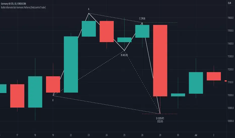
COT-index rangeA graph showing the commercials (part of COT-data) positioning in relation to its own range, X periods back. I usually choose the look-back period to equal approximately one year. This will be around 52 on a weekly chart and 250 on a daily chart.
In my opinion a high data-point for the commercials is bullish and vice versa. But instead of only looking att absolute values I now look more at how the commercials are positioned compared to the previous 12 och 6 months.
Example:
a) if COT-index range = 0.8, then the commercials are in the 80th percentile for this specific look-back period, i.e. the commercials has only been more bullish 20% of the time and more bearish 80% of the time.
b) a) if COT-index range = 0.5, then the commercials are in the 50th percentile for this specific look-back period, i.e. the commercials has been more bullish 50% of the time and more bearish 50% of the time.
c) if COT-index range = 0.2, then the commercials are in the 20th percentile for this specific look-back period, i.e. the commercials has been more bullish 80% of the time and more bearish 20% of the time.
In other words, a high reading is bullish and a low reading is bearish.
Bearish 5-0 Harmonic Patterns [theEccentricTrader]█ OVERVIEW
This indicator automatically draws bearish 5-0 harmonic patterns and price projections derived from the ranges that constitute the patterns.
█ CONCEPTS
Green and Red Candles
• A green candle is one that closes with a close price equal to or above the price it opened.
• A red candle is one that closes with a close price that is lower than the price it opened.
Swing Highs and Swing Lows
• A swing high is a green candle or series of consecutive green candles followed by a single red candle to complete the swing and form the peak.
• A swing low is a red candle or series of consecutive red candles followed by a single green candle to complete the swing and form the trough.
Peak and Trough Prices (Basic)
• The peak price of a complete swing high is the high price of either the red candle that completes the swing high or the high price of the preceding green candle, depending on which is higher.
• The trough price of a complete swing low is the low price of either the green candle that completes the swing low or the low price of the preceding red candle, depending on which is lower.
Historic Peaks and Troughs
The current, or most recent, peak and trough occurrences are referred to as occurrence zero. Previous peak and trough occurrences are referred to as historic and ordered numerically from right to left, with the most recent historic peak and trough occurrences being occurrence one.
Range
The range is simply the difference between the current peak and current trough prices, generally expressed in terms of points or pips.
Support and Resistance
• Support refers to a price level where the demand for an asset is strong enough to prevent the price from falling further.
• Resistance refers to a price level where the supply of an asset is strong enough to prevent the price from rising further.
Support and resistance levels are important because they can help traders identify where the price of an asset might pause or reverse its direction, offering potential entry and exit points. For example, a trader might look to buy an asset when it approaches a support level , with the expectation that the price will bounce back up. Alternatively, a trader might look to sell an asset when it approaches a resistance level , with the expectation that the price will drop back down.
It's important to note that support and resistance levels are not always relevant, and the price of an asset can also break through these levels and continue moving in the same direction.
Upper Trends
• A return line uptrend is formed when the current peak price is higher than the preceding peak price.
• A downtrend is formed when the current peak price is lower than the preceding peak price.
• A double-top is formed when the current peak price is equal to the preceding peak price.
Lower Trends
• An uptrend is formed when the current trough price is higher than the preceding trough price.
• A return line downtrend is formed when the current trough price is lower than the preceding trough price.
• A double-bottom is formed when the current trough price is equal to the preceding trough price.
Muti-Part Upper and Lower Trends
• A multi-part return line uptrend begins with the formation of a new return line uptrend, or higher peak, and continues until a new downtrend, or lower peak, completes the trend.
• A multi-part downtrend begins with the formation of a new downtrend, or lower peak, and continues until a new return line uptrend, or higher peak, completes the trend.
• A multi-part uptrend begins with the formation of a new uptrend, or higher trough, and continues until a new return line downtrend, or lower trough, completes the trend.
• A multi-part return line downtrend begins with the formation of a new return line downtrend, or lower trough, and continues until a new uptrend, or higher trough, completes the trend.
Wave Cycles
A wave cycle is here defined as a complete two-part move between a swing high and a swing low, or a swing low and a swing high. The first swing high or swing low will set the course for the sequence of wave cycles that follow; for example a chart that begins with a swing low will form its first complete wave cycle upon the formation of the first complete swing high and vice versa.
Figure 1.
Fibonacci Retracement and Extension Ratios
The Fibonacci sequence is a series of numbers in which each number is the sum of the two preceding numbers, starting with 0 and 1. For example 0 + 1 = 1, 1 + 1 = 2, 1 + 2 = 3, and so on. Ultimately, we could go on forever but the first few numbers in the sequence are as follows: 0 , 1, 1, 2, 3, 5, 8, 13, 21, 34, 55, 89, 144.
The extension ratios are calculated by dividing each number in the sequence by the number preceding it. For example 0/1 = 0, 1/1 = 1, 2/1 = 2, 3/2 = 1.5, 5/3 = 1.6666..., 8/5 = 1.6, 13/8 = 1.625, 21/13 = 1.6153..., 34/21 = 1.6190..., 55/34 = 1.6176..., 89/55 = 1.6181..., 144/89 = 1.6179..., and so on. The retracement ratios are calculated by inverting this process and dividing each number in the sequence by the number proceeding it. For example 0/1 = 0, 1/1 = 1, 1/2 = 0.5, 2/3 = 0.666..., 3/5 = 0.6, 5/8 = 0.625, 8/13 = 0.6153..., 13/21 = 0.6190..., 21/34 = 0.6176..., 34/55 = 0.6181..., 55/89 = 0.6179..., 89/144 = 0.6180..., and so on.
1.618 is considered to be the 'golden ratio', found in many natural phenomena such as the growth of seashells and the branching of trees. Some now speculate the universe oscillates at a frequency of 0,618 Hz, which could help to explain such phenomena, but this theory has yet to be proven.
Traders and analysts use Fibonacci retracement and extension indicators, consisting of horizontal lines representing different Fibonacci ratios, for identifying potential levels of support and resistance. Fibonacci ranges are typically drawn from left to right, with retracement levels representing ratios inside of the current range and extension levels representing ratios extended outside of the current range. If the current wave cycle ends on a swing low, the Fibonacci range is drawn from peak to trough. If the current wave cycle ends on a swing high the Fibonacci range is drawn from trough to peak.
Harmonic Patterns
The concept of harmonic patterns in trading was first introduced by H.M. Gartley in his book "Profits in the Stock Market", published in 1935. Gartley observed that markets have a tendency to move in repetitive patterns, and he identified several specific patterns that he believed could be used to predict future price movements.
Since then, many other traders and analysts have built upon Gartley's work and developed their own variations of harmonic patterns. One such contributor is Larry Pesavento, who developed his own methods for measuring harmonic patterns using Fibonacci ratios. Pesavento has written several books on the subject of harmonic patterns and Fibonacci ratios in trading. Another notable contributor to harmonic patterns is Scott Carney, who developed his own approach to harmonic trading in the late 1990s and also popularised the use of Fibonacci ratios to measure harmonic patterns. Carney expanded on Gartley's work and also introduced several new harmonic patterns, such as the Shark pattern and the 5-0 pattern.
The bullish and bearish Gartley patterns are the oldest recognized harmonic patterns in trading and all the other harmonic patterns are ultimately modifications of the original Gartley patterns. Gartley patterns are fundamentally composed of 5 points, or 4 waves.
Bullish and Bearish 5-0 Patterns
• Bullish 5-0 patterns are fundamentally composed of three peaks and three troughs, with the second peak being lower than the first peak and the third peak being higher than the first peak. And similarly, the second trough being lower than the first trough and the third trough being higher than both the first and second troughs.
• Bearish 5-0 patterns are fundamentally composed of three troughs and three peaks, with the second trough being higher than the first trough and the third trough being lower than the first trough. And similarly, the second peak being higher than the first peak and the third peak being lower than both the first and second peaks.
The ratio measurements recommended by Scott Carney, who originated the pattern, are as follows:
• Wave 1 of the pattern, referred to as OX, has no specific ratio requirements.
• Wave 2 of the pattern, referred to as XA, has no specific ratio requirements.
• Wave 3 of the pattern, referred to as AB, should extend to at least 113%, but no further than 161.8% of the range set by wave 2.
• Wave 4 of the pattern, referred to as BC, should extend to at least 161.8%, but no further than 224% of the range set by wave 3.
• Wave 5 of the pattern, referred to as CD, should retrace to 50.0% of the range set by wave 4.
Measurement Tolerances
In general, tolerance in measurements refers to the allowable variation or deviation from a specific value or dimension. It is the range within which a particular measurement is considered to be acceptable or accurate. In this script I have applied this concept to the measurement of harmonic pattern ratios to increase to the frequency of pattern occurrences.
For example, the AB measurement of Gartley patterns is generally set at around 61.8%, but with such specificity in the measuring requirements the patterns are very rare. We can increase the frequency of pattern occurrences by setting a tolerance. A tolerance of 10% to both downside and upside, which is the default setting for all tolerances, means we would have a tolerable measurement range between 51.8-71.8%, thus increasing the frequency of occurrence.
█ FEATURES
Inputs
• AB Lower Tolerance
• AB Upper Tolerance
• BC Lower Tolerance
• BC Upper Tolerance
• CD Lower Tolerance
• CD Upper Tolerance
• Pattern Color
• Label Color
• Show Projections
• Extend Current Projection Lines
█ LIMITATIONS
All green and red candle calculations are based on differences between open and close prices, as such I have made no attempt to account for green candles that gap lower and close below the close price of the preceding candle, or red candles that gap higher and close above the close price of the preceding candle. This may cause some unexpected behaviour on some markets and timeframes. I can only recommend using 24-hour markets, if and where possible, as there are far fewer gaps and, generally, more data to work with.
█ NOTES
Here is a link to Scott's harmonic patterns webpage for those who may be interested: harmonictrader.com
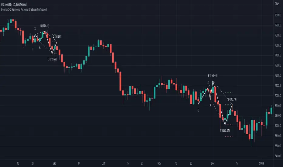
Bullish 5-0 Harmonic Patterns [theEccentricTrader]█ OVERVIEW
This indicator automatically draws bullish 5-0 harmonic patterns and price projections derived from the ranges that constitute the patterns.
█ CONCEPTS
Green and Red Candles
• A green candle is one that closes with a close price equal to or above the price it opened.
• A red candle is one that closes with a close price that is lower than the price it opened.
Swing Highs and Swing Lows
• A swing high is a green candle or series of consecutive green candles followed by a single red candle to complete the swing and form the peak.
• A swing low is a red candle or series of consecutive red candles followed by a single green candle to complete the swing and form the trough.
Peak and Trough Prices (Basic)
• The peak price of a complete swing high is the high price of either the red candle that completes the swing high or the high price of the preceding green candle, depending on which is higher.
• The trough price of a complete swing low is the low price of either the green candle that completes the swing low or the low price of the preceding red candle, depending on which is lower.
Historic Peaks and Troughs
The current, or most recent, peak and trough occurrences are referred to as occurrence zero. Previous peak and trough occurrences are referred to as historic and ordered numerically from right to left, with the most recent historic peak and trough occurrences being occurrence one.
Range
The range is simply the difference between the current peak and current trough prices, generally expressed in terms of points or pips.
Support and Resistance
• Support refers to a price level where the demand for an asset is strong enough to prevent the price from falling further.
• Resistance refers to a price level where the supply of an asset is strong enough to prevent the price from rising further.
Support and resistance levels are important because they can help traders identify where the price of an asset might pause or reverse its direction, offering potential entry and exit points. For example, a trader might look to buy an asset when it approaches a support level , with the expectation that the price will bounce back up. Alternatively, a trader might look to sell an asset when it approaches a resistance level , with the expectation that the price will drop back down.
It's important to note that support and resistance levels are not always relevant, and the price of an asset can also break through these levels and continue moving in the same direction.
Upper Trends
• A return line uptrend is formed when the current peak price is higher than the preceding peak price.
• A downtrend is formed when the current peak price is lower than the preceding peak price.
• A double-top is formed when the current peak price is equal to the preceding peak price.
Lower Trends
• An uptrend is formed when the current trough price is higher than the preceding trough price.
• A return line downtrend is formed when the current trough price is lower than the preceding trough price.
• A double-bottom is formed when the current trough price is equal to the preceding trough price.
Muti-Part Upper and Lower Trends
• A multi-part return line uptrend begins with the formation of a new return line uptrend, or higher peak, and continues until a new downtrend, or lower peak, completes the trend.
• A multi-part downtrend begins with the formation of a new downtrend, or lower peak, and continues until a new return line uptrend, or higher peak, completes the trend.
• A multi-part uptrend begins with the formation of a new uptrend, or higher trough, and continues until a new return line downtrend, or lower trough, completes the trend.
• A multi-part return line downtrend begins with the formation of a new return line downtrend, or lower trough, and continues until a new uptrend, or higher trough, completes the trend.
Wave Cycles
A wave cycle is here defined as a complete two-part move between a swing high and a swing low, or a swing low and a swing high. The first swing high or swing low will set the course for the sequence of wave cycles that follow; for example a chart that begins with a swing low will form its first complete wave cycle upon the formation of the first complete swing high and vice versa.
Figure 1.
Fibonacci Retracement and Extension Ratios
The Fibonacci sequence is a series of numbers in which each number is the sum of the two preceding numbers, starting with 0 and 1. For example 0 + 1 = 1, 1 + 1 = 2, 1 + 2 = 3, and so on. Ultimately, we could go on forever but the first few numbers in the sequence are as follows: 0 , 1, 1, 2, 3, 5, 8, 13, 21, 34, 55, 89, 144.
The extension ratios are calculated by dividing each number in the sequence by the number preceding it. For example 0/1 = 0, 1/1 = 1, 2/1 = 2, 3/2 = 1.5, 5/3 = 1.6666..., 8/5 = 1.6, 13/8 = 1.625, 21/13 = 1.6153..., 34/21 = 1.6190..., 55/34 = 1.6176..., 89/55 = 1.6181..., 144/89 = 1.6179..., and so on. The retracement ratios are calculated by inverting this process and dividing each number in the sequence by the number proceeding it. For example 0/1 = 0, 1/1 = 1, 1/2 = 0.5, 2/3 = 0.666..., 3/5 = 0.6, 5/8 = 0.625, 8/13 = 0.6153..., 13/21 = 0.6190..., 21/34 = 0.6176..., 34/55 = 0.6181..., 55/89 = 0.6179..., 89/144 = 0.6180..., and so on.
1.618 is considered to be the 'golden ratio', found in many natural phenomena such as the growth of seashells and the branching of trees. Some now speculate the universe oscillates at a frequency of 0,618 Hz, which could help to explain such phenomena, but this theory has yet to be proven.
Traders and analysts use Fibonacci retracement and extension indicators, consisting of horizontal lines representing different Fibonacci ratios, for identifying potential levels of support and resistance. Fibonacci ranges are typically drawn from left to right, with retracement levels representing ratios inside of the current range and extension levels representing ratios extended outside of the current range. If the current wave cycle ends on a swing low, the Fibonacci range is drawn from peak to trough. If the current wave cycle ends on a swing high the Fibonacci range is drawn from trough to peak.
Harmonic Patterns
The concept of harmonic patterns in trading was first introduced by H.M. Gartley in his book "Profits in the Stock Market", published in 1935. Gartley observed that markets have a tendency to move in repetitive patterns, and he identified several specific patterns that he believed could be used to predict future price movements.
Since then, many other traders and analysts have built upon Gartley's work and developed their own variations of harmonic patterns. One such contributor is Larry Pesavento, who developed his own methods for measuring harmonic patterns using Fibonacci ratios. Pesavento has written several books on the subject of harmonic patterns and Fibonacci ratios in trading. Another notable contributor to harmonic patterns is Scott Carney, who developed his own approach to harmonic trading in the late 1990s and also popularised the use of Fibonacci ratios to measure harmonic patterns. Carney expanded on Gartley's work and also introduced several new harmonic patterns, such as the Shark pattern and the 5-0 pattern.
The bullish and bearish Gartley patterns are the oldest recognized harmonic patterns in trading and all the other harmonic patterns are ultimately modifications of the original Gartley patterns. Gartley patterns are fundamentally composed of 5 points, or 4 waves.
Bullish and Bearish 5-0 Patterns
• Bullish 5-0 patterns are fundamentally composed of three peaks and three troughs, with the second peak being lower than the first peak and the third peak being higher than the first peak. And similarly, the second trough being lower than the first trough and the third trough being higher than both the first and second troughs.
• Bearish 5-0 patterns are fundamentally composed of three troughs and three peaks, with the second trough being higher than the first trough and the third trough being lower than the first trough. And similarly, the second peak being higher than the first peak and the third peak being lower than both the first and second peaks.
The ratio measurements recommended by Scott Carney, who originated the pattern, are as follows:
• Wave 1 of the pattern, referred to as OX, has no specific ratio requirements.
• Wave 2 of the pattern, referred to as XA, has no specific ratio requirements.
• Wave 3 of the pattern, referred to as AB, should extend to at least 113%, but no further than 161.8% of the range set by wave 2.
• Wave 4 of the pattern, referred to as BC, should extend to at least 161.8%, but no further than 224% of the range set by wave 3.
• Wave 5 of the pattern, referred to as CD, should retrace to 50.0% of the range set by wave 4.
Measurement Tolerances
In general, tolerance in measurements refers to the allowable variation or deviation from a specific value or dimension. It is the range within which a particular measurement is considered to be acceptable or accurate. In this script I have applied this concept to the measurement of harmonic pattern ratios to increase to the frequency of pattern occurrences.
For example, the AB measurement of Gartley patterns is generally set at around 61.8%, but with such specificity in the measuring requirements the patterns are very rare. We can increase the frequency of pattern occurrences by setting a tolerance. A tolerance of 10% to both downside and upside, which is the default setting for all tolerances, means we would have a tolerable measurement range between 51.8-71.8%, thus increasing the frequency of occurrence.
█ FEATURES
Inputs
• AB Lower Tolerance
• AB Upper Tolerance
• BC Lower Tolerance
• BC Upper Tolerance
• CD Lower Tolerance
• CD Upper Tolerance
• Pattern Color
• Label Color
• Show Projections
• Extend Current Projection Lines
█ LIMITATIONS
All green and red candle calculations are based on differences between open and close prices, as such I have made no attempt to account for green candles that gap lower and close below the close price of the preceding candle, or red candles that gap higher and close above the close price of the preceding candle. This may cause some unexpected behaviour on some markets and timeframes. I can only recommend using 24-hour markets, if and where possible, as there are far fewer gaps and, generally, more data to work with.
█ NOTES
Here is a link to Scott's harmonic patterns webpage for those who may be interested: harmonictrader.com

Bearish Shark Harmonic Patterns [theEccentricTrader]█ OVERVIEW
This indicator automatically draws bearish Shark harmonic patterns and price projections derived from the ranges that constitute the patterns.
█ CONCEPTS
Green and Red Candles
• A green candle is one that closes with a close price equal to or above the price it opened.
• A red candle is one that closes with a close price that is lower than the price it opened.
Swing Highs and Swing Lows
• A swing high is a green candle or series of consecutive green candles followed by a single red candle to complete the swing and form the peak.
• A swing low is a red candle or series of consecutive red candles followed by a single green candle to complete the swing and form the trough.
Peak and Trough Prices (Basic)
• The peak price of a complete swing high is the high price of either the red candle that completes the swing high or the high price of the preceding green candle, depending on which is higher.
• The trough price of a complete swing low is the low price of either the green candle that completes the swing low or the low price of the preceding red candle, depending on which is lower.
Historic Peaks and Troughs
The current, or most recent, peak and trough occurrences are referred to as occurrence zero. Previous peak and trough occurrences are referred to as historic and ordered numerically from right to left, with the most recent historic peak and trough occurrences being occurrence one.
Range
The range is simply the difference between the current peak and current trough prices, generally expressed in terms of points or pips.
Support and Resistance
• Support refers to a price level where the demand for an asset is strong enough to prevent the price from falling further.
• Resistance refers to a price level where the supply of an asset is strong enough to prevent the price from rising further.
Support and resistance levels are important because they can help traders identify where the price of an asset might pause or reverse its direction, offering potential entry and exit points. For example, a trader might look to buy an asset when it approaches a support level , with the expectation that the price will bounce back up. Alternatively, a trader might look to sell an asset when it approaches a resistance level , with the expectation that the price will drop back down.
It's important to note that support and resistance levels are not always relevant, and the price of an asset can also break through these levels and continue moving in the same direction.
Upper Trends
• A return line uptrend is formed when the current peak price is higher than the preceding peak price.
• A downtrend is formed when the current peak price is lower than the preceding peak price.
• A double-top is formed when the current peak price is equal to the preceding peak price.
Lower Trends
• An uptrend is formed when the current trough price is higher than the preceding trough price.
• A return line downtrend is formed when the current trough price is lower than the preceding trough price.
• A double-bottom is formed when the current trough price is equal to the preceding trough price.
Muti-Part Upper and Lower Trends
• A multi-part return line uptrend begins with the formation of a new return line uptrend, or higher peak, and continues until a new downtrend, or lower peak, completes the trend.
• A multi-part downtrend begins with the formation of a new downtrend, or lower peak, and continues until a new return line uptrend, or higher peak, completes the trend.
• A multi-part uptrend begins with the formation of a new uptrend, or higher trough, and continues until a new return line downtrend, or lower trough, completes the trend.
• A multi-part return line downtrend begins with the formation of a new return line downtrend, or lower trough, and continues until a new uptrend, or higher trough, completes the trend.
Wave Cycles
A wave cycle is here defined as a complete two-part move between a swing high and a swing low, or a swing low and a swing high. The first swing high or swing low will set the course for the sequence of wave cycles that follow; for example a chart that begins with a swing low will form its first complete wave cycle upon the formation of the first complete swing high and vice versa.
Figure 1.
Fibonacci Retracement and Extension Ratios
The Fibonacci sequence is a series of numbers in which each number is the sum of the two preceding numbers, starting with 0 and 1. For example 0 + 1 = 1, 1 + 1 = 2, 1 + 2 = 3, and so on. Ultimately, we could go on forever but the first few numbers in the sequence are as follows: 0 , 1, 1, 2, 3, 5, 8, 13, 21, 34, 55, 89, 144.
The extension ratios are calculated by dividing each number in the sequence by the number preceding it. For example 0/1 = 0, 1/1 = 1, 2/1 = 2, 3/2 = 1.5, 5/3 = 1.6666..., 8/5 = 1.6, 13/8 = 1.625, 21/13 = 1.6153..., 34/21 = 1.6190..., 55/34 = 1.6176..., 89/55 = 1.6181..., 144/89 = 1.6179..., and so on. The retracement ratios are calculated by inverting this process and dividing each number in the sequence by the number proceeding it. For example 0/1 = 0, 1/1 = 1, 1/2 = 0.5, 2/3 = 0.666..., 3/5 = 0.6, 5/8 = 0.625, 8/13 = 0.6153..., 13/21 = 0.6190..., 21/34 = 0.6176..., 34/55 = 0.6181..., 55/89 = 0.6179..., 89/144 = 0.6180..., and so on.
1.618 is considered to be the 'golden ratio', found in many natural phenomena such as the growth of seashells and the branching of trees. Some now speculate the universe oscillates at a frequency of 0,618 Hz, which could help to explain such phenomena, but this theory has yet to be proven.
Traders and analysts use Fibonacci retracement and extension indicators, consisting of horizontal lines representing different Fibonacci ratios, for identifying potential levels of support and resistance. Fibonacci ranges are typically drawn from left to right, with retracement levels representing ratios inside of the current range and extension levels representing ratios extended outside of the current range. If the current wave cycle ends on a swing low, the Fibonacci range is drawn from peak to trough. If the current wave cycle ends on a swing high the Fibonacci range is drawn from trough to peak.
Harmonic Patterns
The concept of harmonic patterns in trading was first introduced by H.M. Gartley in his book "Profits in the Stock Market", published in 1935. Gartley observed that markets have a tendency to move in repetitive patterns, and he identified several specific patterns that he believed could be used to predict future price movements.
Since then, many other traders and analysts have built upon Gartley's work and developed their own variations of harmonic patterns. One such contributor is Larry Pesavento, who developed his own methods for measuring harmonic patterns using Fibonacci ratios. Pesavento has written several books on the subject of harmonic patterns and Fibonacci ratios in trading. Another notable contributor to harmonic patterns is Scott Carney, who developed his own approach to harmonic trading in the late 1990s and also popularised the use of Fibonacci ratios to measure harmonic patterns. Carney expanded on Gartley's work and also introduced several new harmonic patterns, such as the Shark pattern and the 5-0 pattern.
The bullish and bearish Gartley patterns are the oldest recognized harmonic patterns in trading and all the other harmonic patterns are ultimately modifications of the original Gartley patterns. Gartley patterns are fundamentally composed of 5 points, or 4 waves.
Bullish and Bearish Shark Patterns
• Bullish shark patterns are fundamentally composed of three troughs and two peaks, with the second peak being higher than the first peak and the second trough being higher than the first trough. The third trough must be lower than the second trough but can be above or below the first trough providing it meets the ratio requirements.
• Bearish shark patterns are fundamentally composed of three peaks and two troughs, with the second trough being lower than the first trough and the second peak being lower than the first peak. The third peak must be higher than the second peak but can be above or below the first peak providing it meets the ratio requirements.
The ratio measurements recommended by Scott Carney, who originated the pattern, are as follows:
• Wave 1 of the pattern, referred to as OX, has no specific ratio requirements.
• Wave 2 of the pattern, referred to as XA, has no specific ratio requirements.
• Wave 3 of the pattern, referred to as AB, should extend to at least 113%, but no further than 161.8% of the range set by wave 2.
• Wave 4 of the pattern, referred to as BC, should extend to at least 161.8%, but no further than 224% of the range set by wave 3.
• The last measure, referred to as XC, is that of wave 4 as a ratio of the range set by wave 1, which should extend to at least 88.6%, but no further than 113%.
Measurement Tolerances
In general, tolerance in measurements refers to the allowable variation or deviation from a specific value or dimension. It is the range within which a particular measurement is considered to be acceptable or accurate. In this script I have applied this concept to the measurement of harmonic pattern ratios to increase to the frequency of pattern occurrences.
For example, the AB measurement of Gartley patterns is generally set at around 61.8%, but with such specificity in the measuring requirements the patterns are very rare. We can increase the frequency of pattern occurrences by setting a tolerance. A tolerance of 10% to both downside and upside, which is the default setting for all tolerances, means we would have a tolerable measurement range between 51.8-71.8%, thus increasing the frequency of occurrence.
█ FEATURES
Inputs
• AB Lower Tolerance
• AB Upper Tolerance
• BC Lower Tolerance
• BC Upper Tolerance
• XC Lower Tolerance
• XC Upper Tolerance
• Pattern Color
• Label Color
• Show Projections
• Extend Current Projection Lines
█ LIMITATIONS
All green and red candle calculations are based on differences between open and close prices, as such I have made no attempt to account for green candles that gap lower and close below the close price of the preceding candle, or red candles that gap higher and close above the close price of the preceding candle. This may cause some unexpected behaviour on some markets and timeframes. I can only recommend using 24-hour markets, if and where possible, as there are far fewer gaps and, generally, more data to work with.
█ NOTES
Here is a link to Scott's harmonic patterns webpage for those who may be interested: harmonictrader.com
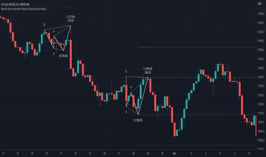
Bullish Shark Harmonic Patterns [theEccentricTrader]█ OVERVIEW
This indicator automatically draws bullish Shark harmonic patterns and price projections derived from the ranges that constitute the patterns.
█ CONCEPTS
Green and Red Candles
• A green candle is one that closes with a close price equal to or above the price it opened.
• A red candle is one that closes with a close price that is lower than the price it opened.
Swing Highs and Swing Lows
• A swing high is a green candle or series of consecutive green candles followed by a single red candle to complete the swing and form the peak.
• A swing low is a red candle or series of consecutive red candles followed by a single green candle to complete the swing and form the trough.
Peak and Trough Prices (Basic)
• The peak price of a complete swing high is the high price of either the red candle that completes the swing high or the high price of the preceding green candle, depending on which is higher.
• The trough price of a complete swing low is the low price of either the green candle that completes the swing low or the low price of the preceding red candle, depending on which is lower.
Historic Peaks and Troughs
The current, or most recent, peak and trough occurrences are referred to as occurrence zero. Previous peak and trough occurrences are referred to as historic and ordered numerically from right to left, with the most recent historic peak and trough occurrences being occurrence one.
Range
The range is simply the difference between the current peak and current trough prices, generally expressed in terms of points or pips.
Support and Resistance
• Support refers to a price level where the demand for an asset is strong enough to prevent the price from falling further.
• Resistance refers to a price level where the supply of an asset is strong enough to prevent the price from rising further.
Support and resistance levels are important because they can help traders identify where the price of an asset might pause or reverse its direction, offering potential entry and exit points. For example, a trader might look to buy an asset when it approaches a support level , with the expectation that the price will bounce back up. Alternatively, a trader might look to sell an asset when it approaches a resistance level , with the expectation that the price will drop back down.
It's important to note that support and resistance levels are not always relevant, and the price of an asset can also break through these levels and continue moving in the same direction.
Upper Trends
• A return line uptrend is formed when the current peak price is higher than the preceding peak price.
• A downtrend is formed when the current peak price is lower than the preceding peak price.
• A double-top is formed when the current peak price is equal to the preceding peak price.
Lower Trends
• An uptrend is formed when the current trough price is higher than the preceding trough price.
• A return line downtrend is formed when the current trough price is lower than the preceding trough price.
• A double-bottom is formed when the current trough price is equal to the preceding trough price.
Muti-Part Upper and Lower Trends
• A multi-part return line uptrend begins with the formation of a new return line uptrend, or higher peak, and continues until a new downtrend, or lower peak, completes the trend.
• A multi-part downtrend begins with the formation of a new downtrend, or lower peak, and continues until a new return line uptrend, or higher peak, completes the trend.
• A multi-part uptrend begins with the formation of a new uptrend, or higher trough, and continues until a new return line downtrend, or lower trough, completes the trend.
• A multi-part return line downtrend begins with the formation of a new return line downtrend, or lower trough, and continues until a new uptrend, or higher trough, completes the trend.
Wave Cycles
A wave cycle is here defined as a complete two-part move between a swing high and a swing low, or a swing low and a swing high. The first swing high or swing low will set the course for the sequence of wave cycles that follow; for example a chart that begins with a swing low will form its first complete wave cycle upon the formation of the first complete swing high and vice versa.
Figure 1.
Fibonacci Retracement and Extension Ratios
The Fibonacci sequence is a series of numbers in which each number is the sum of the two preceding numbers, starting with 0 and 1. For example 0 + 1 = 1, 1 + 1 = 2, 1 + 2 = 3, and so on. Ultimately, we could go on forever but the first few numbers in the sequence are as follows: 0 , 1, 1, 2, 3, 5, 8, 13, 21, 34, 55, 89, 144.
The extension ratios are calculated by dividing each number in the sequence by the number preceding it. For example 0/1 = 0, 1/1 = 1, 2/1 = 2, 3/2 = 1.5, 5/3 = 1.6666..., 8/5 = 1.6, 13/8 = 1.625, 21/13 = 1.6153..., 34/21 = 1.6190..., 55/34 = 1.6176..., 89/55 = 1.6181..., 144/89 = 1.6179..., and so on. The retracement ratios are calculated by inverting this process and dividing each number in the sequence by the number proceeding it. For example 0/1 = 0, 1/1 = 1, 1/2 = 0.5, 2/3 = 0.666..., 3/5 = 0.6, 5/8 = 0.625, 8/13 = 0.6153..., 13/21 = 0.6190..., 21/34 = 0.6176..., 34/55 = 0.6181..., 55/89 = 0.6179..., 89/144 = 0.6180..., and so on.
1.618 is considered to be the 'golden ratio', found in many natural phenomena such as the growth of seashells and the branching of trees. Some now speculate the universe oscillates at a frequency of 0,618 Hz, which could help to explain such phenomena, but this theory has yet to be proven.
Traders and analysts use Fibonacci retracement and extension indicators, consisting of horizontal lines representing different Fibonacci ratios, for identifying potential levels of support and resistance. Fibonacci ranges are typically drawn from left to right, with retracement levels representing ratios inside of the current range and extension levels representing ratios extended outside of the current range. If the current wave cycle ends on a swing low, the Fibonacci range is drawn from peak to trough. If the current wave cycle ends on a swing high the Fibonacci range is drawn from trough to peak.
Harmonic Patterns
The concept of harmonic patterns in trading was first introduced by H.M. Gartley in his book "Profits in the Stock Market", published in 1935. Gartley observed that markets have a tendency to move in repetitive patterns, and he identified several specific patterns that he believed could be used to predict future price movements.
Since then, many other traders and analysts have built upon Gartley's work and developed their own variations of harmonic patterns. One such contributor is Larry Pesavento, who developed his own methods for measuring harmonic patterns using Fibonacci ratios. Pesavento has written several books on the subject of harmonic patterns and Fibonacci ratios in trading. Another notable contributor to harmonic patterns is Scott Carney, who developed his own approach to harmonic trading in the late 1990s and also popularised the use of Fibonacci ratios to measure harmonic patterns. Carney expanded on Gartley's work and also introduced several new harmonic patterns, such as the Shark pattern and the 5-0 pattern.
The bullish and bearish Gartley patterns are the oldest recognized harmonic patterns in trading and all the other harmonic patterns are ultimately modifications of the original Gartley patterns. Gartley patterns are fundamentally composed of 5 points, or 4 waves.
Bullish and Bearish Shark Patterns
• Bullish shark patterns are fundamentally composed of three troughs and two peaks, with the second peak being higher than the first peak and the second trough being higher than the first trough. The third trough must be lower than the second trough but can be above or below the first trough providing it meets the ratio requirements.
• Bearish shark patterns are fundamentally composed of three peaks and two troughs, with the second trough being lower than the first trough and the second peak being lower than the first peak. The third peak must be higher than the second peak but can be above or below the first peak providing it meets the ratio requirements.
The ratio measurements recommended by Scott Carney, who originated the pattern, are as follows:
• Wave 1 of the pattern, referred to as OX, has no specific ratio requirements.
• Wave 2 of the pattern, referred to as XA, has no specific ratio requirements.
• Wave 3 of the pattern, referred to as AB, should extend to at least 113%, but no further than 161.8% of the range set by wave 2.
• Wave 4 of the pattern, referred to as BC, should extend to at least 161.8%, but no further than 224% of the range set by wave 3.
• The last measure, referred to as XC, is that of wave 4 as a ratio of the range set by wave 1, which should extend to at least 88.6%, but no further than 113%.
Measurement Tolerances
In general, tolerance in measurements refers to the allowable variation or deviation from a specific value or dimension. It is the range within which a particular measurement is considered to be acceptable or accurate. In this script I have applied this concept to the measurement of harmonic pattern ratios to increase to the frequency of pattern occurrences.
For example, the AB measurement of Gartley patterns is generally set at around 61.8%, but with such specificity in the measuring requirements the patterns are very rare. We can increase the frequency of pattern occurrences by setting a tolerance. A tolerance of 10% to both downside and upside, which is the default setting for all tolerances, means we would have a tolerable measurement range between 51.8-71.8%, thus increasing the frequency of occurrence.
█ FEATURES
Inputs
• AB Lower Tolerance
• AB Upper Tolerance
• BC Lower Tolerance
• BC Upper Tolerance
• XC Lower Tolerance
• XC Upper Tolerance
• Pattern Color
• Label Color
• Show Projections
• Extend Current Projection Lines
█ LIMITATIONS
All green and red candle calculations are based on differences between open and close prices, as such I have made no attempt to account for green candles that gap lower and close below the close price of the preceding candle, or red candles that gap higher and close above the close price of the preceding candle. This may cause some unexpected behaviour on some markets and timeframes. I can only recommend using 24-hour markets, if and where possible, as there are far fewer gaps and, generally, more data to work with.
█ NOTES
Here is a link to Scott's harmonic patterns webpage for those who may be interested: harmonictrader.com