Поиск скриптов по запросу "马斯克+100万"
BB 100 with Barcolors6/19/15 I added confirmation highlight bars to the code. In other words, if a candle bounced off the lower Bollinger band, it needed one more close above the previous candle to confirm a higher probability that a change in investor sentiment has reversed. Same is true for upper Bollinger band bounces. I also added confirmation highlight bars to the 100 sma (the basis). The idea is that lower and upper bands are potential points of support and resistance. The same is true of the basis if a trend is to continue. 6/28/15 I added a plotshape to identify closes above/below TLine. One thing this system points out is it operates best in a trend reversal. Consolidations will whipsaw the indicator too much. I have found that when this happens, if using daily candles, switch to hourly, 30 min, etc., to catch a better signal. Nothing moves in a straight line. As with any indicator, it is a tool to be used in conjunction with the art AND science of trading. As always, try the indicator for a time so that you are comfortable enough to use real money. This is designed to be used with "BB 25 with Barcolors".

BB 100 with Barcolors6/19/15 I added confirmation highlight bars to the code. In other words, if a candle bounced off the lower Bollinger band, it needed one more close above the previous candle to confirm a higher probability that a change in investor sentiment has reversed. Same is true for upper Bollinger band bounces. I also added confirmation highlight bars to the 100 sma (the basis). The idea is that lower and upper bands are potential points of support and resistance. The same is true of the basis if a trend is to continue. Nothing moves in a straight line. As with any indicator, it is a tool to be used in conjunction with the art AND science of trading. As always, try the indicator for a time so that you are comfortable enough to use real money. This is designed to be used with "BB 25 with Barcolors".
BB 100 with BarcolorsI cleaned up the highlight barcolor to reflect red or lime depending if it closed > or < the open.
The description is in the code. you want to catch bounces off the 25 (upper or lower) and 100 (upper or lower).
Works well on the hourly and 30 min charts. Haven't tested it beyond that. Haven't tested Forex, just equities.

EMA Keltner Channel 1D100/200 EMAs, along with Keltner Bands based off them. Colors correspond to actions you should be ready to take in the area. Use to set macro mindset.
Uses the security function to display only the 1D values.
Red= Bad
Orange = Not as Bad, but still Bad.
Yellow = Warning, might also be Bad.
Purple = Dip a toe in.
Blue = Give it a shot but have a little caution.
Green = It's second mortgage time.
Advanced Speedometer Gauge [PhenLabs]Advanced Speedometer Gauge
Version: PineScript™v6
📌 Description
The Advanced Speedometer Gauge is a revolutionary multi-metric visualization tool that consolidates 13 distinct trading indicators into a single, intuitive speedometer display. Instead of cluttering your workspace with multiple oscillators and panels, this gauge provides a unified interface where you can switch between different metrics while maintaining consistent visual interpretation.
Built on PineScript™ v6, the indicator transforms complex technical calculations into an easy-to-read semi-circular gauge with color-coded zones and a precision needle indicator. Each of the 13 available metrics has been carefully normalized to a 0-100 scale, ensuring that whether you’re analyzing RSI, volume trends, or volatility extremes, the visual interpretation remains consistent and intuitive.
The gauge is designed for traders who value efficiency and clarity. By consolidating multiple analytical perspectives into one compact display, you can quickly assess market conditions without the visual noise of traditional multi-indicator setups. All metrics are non-overlapping, meaning each provides unique insights into different aspects of market behavior.
🚀 Points of Innovation
13 selectable metrics covering momentum, volume, volatility, trend, and statistical analysis, all accessible through a single dropdown menu
Universal 0-100 normalization system that standardizes different indicator scales for consistent visual interpretation across all metrics
Semi-circular gauge design with 21 arc segments providing smooth precision and clear visual feedback through color-coded zones
Non-redundant metric selection ensuring each indicator provides unique market insights without analytical overlap
Advanced metrics including MFI (volume-weighted momentum), CCI (statistical deviation), Volatility Rank (extended lookback), Trend Strength (ADX-style), Choppiness Index, Volume Trend, and Price Distance from MA
Flexible positioning system with 5 chart locations, 3 size options, and fully customizable color schemes for optimal workspace integration
🔧 Core Components
Metric Selection Engine: Dropdown interface allowing instant switching between 13 different technical indicators, each with independent parameter controls
Normalization System: All metrics converted to 0-100 scale using indicator-specific algorithms that preserve the statistical significance of each measurement
Semi-Circular Gauge: Visual display using 21 arc segments arranged in curved formation with two-row thickness for enhanced visibility
Color Zone System: Three distinct zones (0-40 green, 40-70 yellow, 70-100 red) providing instant visual feedback on metric extremes
Needle Indicator: Dynamic pointer that positions across the gauge arc based on precise current metric value
Table Implementation: Professional table structure ensuring consistent positioning and rendering across different chart configurations
🔥 Key Features
RSI (Relative Strength Index): Classic momentum oscillator measuring overbought/oversold conditions with adjustable period length (default 14)
Stochastic Oscillator: Compares closing price to price range over specified period with smoothing, ideal for identifying momentum shifts
MFI (Money Flow Index): Volume-weighted RSI that combines price movement with volume to measure buying and selling pressure intensity
CCI (Commodity Channel Index): Measures statistical deviation from average price, normalized from typical -200 to +200 range to 0-100 scale
Williams %R: Alternative overbought/oversold indicator using high-low range analysis, inverted to match 0-100 scale conventions
Volume %: Current volume relative to moving average expressed as percentage, capped at 100 for extreme spikes
Volume Trend: Cumulative directional volume flow showing whether volume is flowing into up moves or down moves over specified period
ATR Percentile: Current Average True Range position within historical range using specified lookback period (default 100 bars)
Volatility Rank: Close-to-close volatility measured against extended historical range (default 252 days), differs from ATR in calculation method
Momentum: Rate of change calculation showing price movement speed, centered at 50 and normalized to 0-100 range
Trend Strength: ADX-style calculation using directional movement to quantify trend intensity regardless of direction
Choppiness Index: Measures market choppiness versus trending behavior, where high values indicate ranging markets and low values indicate strong trends
Price Distance from MA: Measures current price over-extension from moving average using standard deviation calculations
🎨 Visualization
Semi-Circular Arc Display: Curved gauge spanning from 0 (left) to 100 (right) with smooth progression and two-row thickness for visibility
Color-Coded Zones: Green zone (0-40) for low/oversold conditions, yellow zone (40-70) for neutral readings, red zone (70-100) for high/overbought conditions
Needle Indicator: Downward-pointing triangle (▼) positioned precisely at current metric value along the gauge arc
Scale Markers: Vertical line markers at 0, 25, 50, 75, and 100 positions with corresponding numerical labels below
Title Display: Merged cell showing “𓄀 PhenLabs” branding plus currently selected metric name in monospace font
Large Value Display: Current metric value shown with two decimal precision in large text directly below title
Table Structure: Professional table with customizable background color, text color, and transparency for minimal chart obstruction
📖 Usage Guidelines
Metric Selection
Select Metric: Default: RSI | Options: RSI, Stochastic, Volume %, ATR Percentile, Momentum, MFI (Money Flow), CCI (Commodity Channel), Williams %R, Volatility Rank, Trend Strength, Choppiness Index, Volume Trend, Price Distance | Choose the technical indicator you want to display on the gauge based on your current analytical needs
RSI Settings
RSI Length: Default: 14 | Range: 1+ | Controls the lookback period for RSI calculation, shorter periods increase sensitivity to recent price changes
Stochastic Settings
Stochastic Length: Default: 14 | Range: 1+ | Lookback period for stochastic calculation comparing close to high-low range
Stochastic Smooth: Default: 3 | Range: 1+ | Smoothing period applied to raw stochastic value to reduce noise and false signals
Volume Settings
Volume MA Length: Default: 20 | Range: 1+ | Moving average period used to calculate average volume for comparison with current volume
Volume Trend Length: Default: 20 | Range: 5+ | Period for calculating cumulative directional volume flow trend
ATR and Volatility Settings
ATR Length: Default: 14 | Range: 1+ | Period for Average True Range calculation used in ATR Percentile metric
ATR Percentile Lookback: Default: 100 | Range: 20+ | Historical range used to determine current ATR position as percentile
Volatility Rank Lookback (Days): Default: 252 | Range: 50+ | Extended lookback period for Volatility Rank metric using close-to-close volatility
Momentum and Trend Settings
Momentum Length: Default: 10 | Range: 1+ | Lookback period for rate of change calculation in Momentum metric
Trend Strength Length: Default: 20 | Range: 5+ | Period for directional movement calculations in ADX-style Trend Strength metric
Advanced Metric Settings
MFI Length: Default: 14 | Range: 1+ | Lookback period for Money Flow Index calculation combining price and volume
CCI Length: Default: 20 | Range: 1+ | Period for Commodity Channel Index statistical deviation calculation
Williams %R Length: Default: 14 | Range: 1+ | Lookback period for Williams %R high-low range analysis
Choppiness Index Length: Default: 14 | Range: 5+ | Period for calculating market choppiness versus trending behavior
Price Distance MA Length: Default: 50 | Range: 10+ | Moving average period used for Price Distance standard deviation calculation
Visual Customization
Position: Default: Top Right | Options: Top Left, Top Right, Bottom Left, Bottom Right, Middle Right | Controls gauge placement on chart for optimal workspace organization
Size: Default: Normal | Options: Small, Normal, Large | Adjusts overall gauge dimensions and text size for different monitor resolutions and preferences
Low Zone Color (0-40): Default: Green (#00FF00) | Customize color for low/oversold zone of gauge arc
Medium Zone Color (40-70): Default: Yellow (#FFFF00) | Customize color for neutral/medium zone of gauge arc
High Zone Color (70-100): Default: Red (#FF0000) | Customize color for high/overbought zone of gauge arc
Background Color: Default: Semi-transparent dark gray | Customize gauge background for contrast and chart integration
Text Color: Default: White (#FFFFFF) | Customize all text elements including title, value, and scale labels
✅ Best Use Cases
Quick visual assessment of market conditions when you need instant feedback on whether an asset is in extreme territory across multiple analytical dimensions
Workspace organization for traders who monitor multiple indicators but want to reduce chart clutter and visual complexity
Metric comparison by switching between different indicators while maintaining consistent visual interpretation through the 0-100 normalization
Overbought/oversold identification using RSI, Stochastic, Williams %R, or MFI depending on whether you prefer price-only or volume-weighted analysis
Volume analysis through Volume %, Volume Trend, or MFI to confirm price movements with corresponding volume characteristics
Volatility monitoring using ATR Percentile or Volatility Rank to identify expansion/contraction cycles and adjust position sizing
Trend vs range identification by comparing Trend Strength (high values = trending) against Choppiness Index (high values = ranging)
Statistical over-extension detection using CCI or Price Distance to identify when price has deviated significantly from normal behavior
Multi-timeframe analysis by duplicating the gauge on different timeframe charts to compare metric readings across time horizons
Educational purposes for new traders learning to interpret technical indicators through consistent visual representation
⚠️ Limitations
The gauge displays only one metric at a time, requiring manual switching to compare different indicators rather than simultaneous multi-metric viewing
The 0-100 normalization, while providing consistency, may obscure the raw values and specific nuances of each underlying indicator
Table-based visualization cannot be exported or saved as an image separately from the full chart screenshot
Optimal parameter settings vary by asset type, timeframe, and market conditions, requiring user experimentation for best results
💡 What Makes This Unique
Unified Multi-Metric Interface: The only gauge-style indicator offering 13 distinct metrics through a single interface, eliminating the need for multiple oscillator panels
Non-Overlapping Analytics: Each metric provides genuinely unique insights—MFI combines volume with price, CCI measures statistical deviation, Volatility Rank uses extended lookback, Trend Strength quantifies directional movement, and Choppiness Index measures ranging behavior
Universal Normalization System: All metrics standardized to 0-100 scale using indicator-appropriate algorithms that preserve statistical meaning while enabling consistent visual interpretation
Professional Visual Design: Semi-circular gauge with 21 arc segments, precision needle positioning, color-coded zones, and clean table implementation that maintains clarity across all chart configurations
Extensive Customization: Independent parameter controls for each metric, five position options, three size presets, and full color customization for seamless workspace integration
🔬 How It Works
1. Metric Calculation Phase:
All 13 metrics are calculated simultaneously on every bar using their respective algorithms with user-defined parameters
Each metric applies its own specific calculation method—RSI uses average gains vs losses, Stochastic compares close to high-low range, MFI incorporates typical price and volume, CCI measures deviation from statistical mean, ATR calculates true range, directional indicators measure up/down movement, and statistical metrics analyze price relationships
2. Normalization Process:
Each calculated metric is converted to a standardized 0-100 scale using indicator-appropriate transformations
Some metrics are naturally 0-100 (RSI, Stochastic, MFI, Williams %R), while others require scaling—CCI transforms from ±200 range, Momentum centers around 50, Volume ratio caps at 2x for 100, ATR and Volatility Rank calculate percentile positions, and Price Distance scales by standard deviations
3. Gauge Rendering:
The selected metric’s normalized value determines the needle position across 21 arc segments spanning 0-100
Each arc segment receives its color based on position—segments 0-8 are green zone, segments 9-14 are yellow zone, segments 15-20 are red zone
The needle indicator (▼) appears in row 5 at the column corresponding to the current metric value, providing precise visual feedback
4. Table Construction:
The gauge uses TradingView’s table system with merged cells for title and value display, ensuring consistent positioning regardless of chart configuration
Rows are allocated as follows: Row 0 merged for title, Row 1 merged for large value display, Row 2 for spacing, Rows 3-4 for the semi-circular arc with curved shaping, Row 5 for needle indicator, Row 6 for scale markers, Row 7 for numerical labels at 0/25/50/75/100
All visual elements update on every bar when barstate.islast is true, ensuring real-time accuracy without performance impact
💡 Note:
This indicator is designed for visual analysis and market condition assessment, not as a standalone trading system. For best results, combine gauge readings with price action analysis, support and resistance levels, and broader market context. Parameter optimization is recommended based on your specific trading timeframe and asset class. The gauge works on all timeframes but may require different parameter settings for intraday versus daily/weekly analysis. Consider using multiple instances of the gauge set to different metrics for comprehensive market analysis without switching between settings.

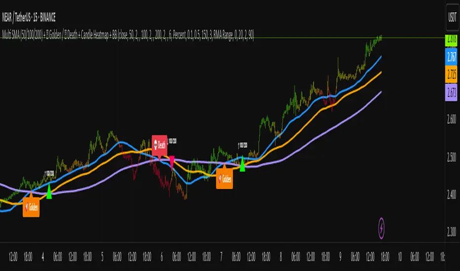
Multi SMA + Golden/Death + Heatmap + BB**Multi SMA (50/100/200) + Golden/Death + Candle Heatmap + BB**
A practical trend toolkit that blends classic 50/100/200 SMAs with clear crossover labels, special 🚀 Golden / 💀 Death Cross markers, and a readable candle heatmap based on a dynamic regression midline and volatility bands. Optional Bollinger Bands are included for context.
* See trend direction at a glance with SMAs.
* Get minimal, de-cluttered labels on important crosses (50↔100, 50↔200, 100↔200).
* Highlight big regime shifts with special Golden/Death tags.
* Read momentum and volatility with the candle heatmap.
* Add Bollinger Bands if you want classic mean-reversion context.
Designed to be lightweight, non-repainting on confirmed bars, and flexible across timeframes.
# What This Indicator Does (plain English)
* **Tracks trend** using **SMA 50/100/200** and lets you optionally compute each SMA on a higher or different timeframe (HTF-safe, no lookahead).
* **Prints labels** when SMAs cross each other (up or down). You can force signals only after bar close to avoid repaint.
* **Marks Golden/Death Crosses** (50 over/under 200) with special labels so major regime changes stand out.
* **Colors candles** with a **heatmap** built from a regression midline and volatility bands—greenish above, reddish below, with a smooth gradient.
* **Optionally shows Bollinger Bands** (basis SMA + stdev bands) and fills the area between them.
* **Includes alert conditions** for Golden and Death Cross so you can automate notifications.
---
# Settings — Simple Explanations
## Source
* **Source**: Price source used to calculate SMAs and Bollinger basis. Default: `close`.
## SMA 50
* **Show 50**: Turn the SMA(50) line on/off.
* **Length 50**: How many bars to average. Lower = faster but noisier.
* **Color 50** / **Width 50**: Visual style.
* **Timeframe 50**: Optional alternate timeframe for SMA(50). Leave empty to use the chart timeframe.
## SMA 100
* **Show 100**: Turn the SMA(100) line on/off.
* **Length 100**: Bars used for the mid-term trend.
* **Color 100** / **Width 100**: Visual style.
* **Timeframe 100**: Optional alternate timeframe for SMA(100).
## SMA 200
* **Show 200**: Turn the SMA(200) line on/off.
* **Length 200**: Bars used for the long-term trend.
* **Color 200** / **Width 200**: Visual style.
* **Timeframe 200**: Optional alternate timeframe for SMA(200).
## Signals (crossover labels)
* **Show crossover signals**: Prints triangle labels on SMA crosses (50↔100, 50↔200, 100↔200).
* **Wait for bar close (confirmed)**: If ON, signals only appear after the candle closes (reduces repaint).
* **Min bars between same-pair signals**: Minimum spacing to avoid duplicate labels from the same SMA pair too often.
* **Trend filter (buy: 50>100>200, sell: 50<100<200)**: Only show bullish labels when SMAs are stacked bullish (50 above 100 above 200), and only show bearish labels when stacked bearish.
### Label Offset
* **Offset mode**: Choose how to push labels away from price:
* **Percent**: Offset is a % of price.
* **ATR x**: Offset is ATR(14) × multiplier.
* **Percent of price (%)**: Used when mode = Percent.
* **ATR multiplier (for ‘ATR x’)**: Used when mode = ATR x.
### Label Colors
* **Bull color** / **Bear color**: Background of triangle labels.
* **Bull label text color** / **Bear label text color**: Text color inside the triangles.
## Golden / Death Cross
* **Show 🚀 Golden Cross (50↑200)**: Show a special “Golden” label when SMA50 crosses above SMA200.
* **Golden label color** / **Golden text color**: Styling for Golden label.
* **Show 💀 Death Cross (50↓200)**: Show a special “Death” label when SMA50 crosses below SMA200.
* **Death label color** / **Death text color**: Styling for Death label.
## Candle Heatmap
* **Enable heatmap candle colors**: Turns the heatmap on/off.
* **Length**: Lookback for the regression midline and volatility measure.
* **Deviation Multiplier**: Band width around the midline (bigger = wider).
* **Volatility basis**:
* **RMA Range** (smoothed high-low range)
* **Stdev** (standard deviation of close)
* **Upper/Middle/Lower color**: Gradient colors for the heatmap.
* **Heatmap transparency (0..100)**: 0 = solid, 100 = invisible.
* **Force override base candles**: Repaint base candles so heatmap stays visible even if your chart has custom coloring.
## Bollinger Bands (optional)
* **Show Bollinger Bands**: Toggle the overlay on/off.
* **Length**: Basis SMA length.
* **StdDev Multiplier**: Distance of bands from the basis in standard deviations.
* **Basis color** / **Band color**: Line colors for basis and bands.
* **Bands fill transparency**: Opacity of the fill between upper/lower bands.
---
# Features & How It Works
## 1) HTF-Safe SMAs
Each SMA can be calculated on the chart timeframe or a higher/different timeframe you choose. The script pulls HTF values **without lookahead** (non-repainting on confirmed bars).
## 2) Crossover Labels (Three Pairs)
* **50↔100**, **50↔200**, **100↔200**:
* **Triangle Up** label when the first SMA crosses **above** the second.
* **Triangle Down** label when it crosses **below**.
* Optional **Trend Filter** ensures only signals aligned with the overall stack (50>100>200 for bullish, 50<100<200 for bearish).
* **Debounce** spacing avoids repeated labels for the same pair too close together.
## 3) Golden / Death Cross Highlights
* **🚀 Golden Cross**: SMA50 crosses **above** SMA200 (often a longer-term bullish regime shift).
* **💀 Death Cross**: SMA50 crosses **below** SMA200 (often a longer-term bearish regime shift).
* Separate styling so they stand out from regular cross labels.
## 4) Candle Heatmap
* Builds a **regression midline** with **volatility bands**; colors candles by their position inside that channel.
* Smooth gradient: lower side → reddish, mid → yellowish, upper side → greenish.
* Helps you see momentum and “where price sits” relative to a dynamic channel.
## 5) Bollinger Bands (Optional)
* Classic **basis SMA** ± **StdDev** bands.
* Light visual context for mean-reversion and volatility expansion.
## 6) Alerts
* **Golden Cross**: `🚀 GOLDEN CROSS: SMA 50 crossed ABOVE SMA 200`
* **Death Cross**: `💀 DEATH CROSS: SMA 50 crossed BELOW SMA 200`
Add these to your alerts to get notified automatically.
---
# Tips & Notes
* For fewer false positives, keep **“Wait for bar close”** ON, especially on lower timeframes.
* Use the **Trend Filter** to align signals with the broader stack and cut noise.
* For HTF context, set **Timeframe 50/100/200** to higher frames (e.g., H1/H4/D) while you trade on a lower frame.
* Heatmap “Length” and “Deviation Multiplier” control smoothness and channel width—tune for your asset’s volatility.
Markov Chain [3D] | FractalystWhat exactly is a Markov Chain?
This indicator uses a Markov Chain model to analyze, quantify, and visualize the transitions between market regimes (Bull, Bear, Neutral) on your chart. It dynamically detects these regimes in real-time, calculates transition probabilities, and displays them as animated 3D spheres and arrows, giving traders intuitive insight into current and future market conditions.
How does a Markov Chain work, and how should I read this spheres-and-arrows diagram?
Think of three weather modes: Sunny, Rainy, Cloudy.
Each sphere is one mode. The loop on a sphere means “stay the same next step” (e.g., Sunny again tomorrow).
The arrows leaving a sphere show where things usually go next if they change (e.g., Sunny moving to Cloudy).
Some paths matter more than others. A more prominent loop means the current mode tends to persist. A more prominent outgoing arrow means a change to that destination is the usual next step.
Direction isn’t symmetric: moving Sunny→Cloudy can behave differently than Cloudy→Sunny.
Now relabel the spheres to markets: Bull, Bear, Neutral.
Spheres: market regimes (uptrend, downtrend, range).
Self‑loop: tendency for the current regime to continue on the next bar.
Arrows: the most common next regime if a switch happens.
How to read: Start at the sphere that matches current bar state. If the loop stands out, expect continuation. If one outgoing path stands out, that switch is the typical next step. Opposite directions can differ (Bear→Neutral doesn’t have to match Neutral→Bear).
What states and transitions are shown?
The three market states visualized are:
Bullish (Bull): Upward or strong-market regime.
Bearish (Bear): Downward or weak-market regime.
Neutral: Sideways or range-bound regime.
Bidirectional animated arrows and probability labels show how likely the market is to move from one regime to another (e.g., Bull → Bear or Neutral → Bull).
How does the regime detection system work?
You can use either built-in price returns (based on adaptive Z-score normalization) or supply three custom indicators (such as volume, oscillators, etc.).
Values are statistically normalized (Z-scored) over a configurable lookback period.
The normalized outputs are classified into Bull, Bear, or Neutral zones.
If using three indicators, their regime signals are averaged and smoothed for robustness.
How are transition probabilities calculated?
On every confirmed bar, the algorithm tracks the sequence of detected market states, then builds a rolling window of transitions.
The code maintains a transition count matrix for all regime pairs (e.g., Bull → Bear).
Transition probabilities are extracted for each possible state change using Laplace smoothing for numerical stability, and frequently updated in real-time.
What is unique about the visualization?
3D animated spheres represent each regime and change visually when active.
Animated, bidirectional arrows reveal transition probabilities and allow you to see both dominant and less likely regime flows.
Particles (moving dots) animate along the arrows, enhancing the perception of regime flow direction and speed.
All elements dynamically update with each new price bar, providing a live market map in an intuitive, engaging format.
Can I use custom indicators for regime classification?
Yes! Enable the "Custom Indicators" switch and select any three chart series as inputs. These will be normalized and combined (each with equal weight), broadening the regime classification beyond just price-based movement.
What does the “Lookback Period” control?
Lookback Period (default: 100) sets how much historical data builds the probability matrix. Shorter periods adapt faster to regime changes but may be noisier. Longer periods are more stable but slower to adapt.
How is this different from a Hidden Markov Model (HMM)?
It sets the window for both regime detection and probability calculations. Lower values make the system more reactive, but potentially noisier. Higher values smooth estimates and make the system more robust.
How is this Markov Chain different from a Hidden Markov Model (HMM)?
Markov Chain (as here): All market regimes (Bull, Bear, Neutral) are directly observable on the chart. The transition matrix is built from actual detected regimes, keeping the model simple and interpretable.
Hidden Markov Model: The actual regimes are unobservable ("hidden") and must be inferred from market output or indicator "emissions" using statistical learning algorithms. HMMs are more complex, can capture more subtle structure, but are harder to visualize and require additional machine learning steps for training.
A standard Markov Chain models transitions between observable states using a simple transition matrix, while a Hidden Markov Model assumes the true states are hidden (latent) and must be inferred from observable “emissions” like price or volume data. In practical terms, a Markov Chain is transparent and easier to implement and interpret; an HMM is more expressive but requires statistical inference to estimate hidden states from data.
Markov Chain: states are observable; you directly count or estimate transition probabilities between visible states. This makes it simpler, faster, and easier to validate and tune.
HMM: states are hidden; you only observe emissions generated by those latent states. Learning involves machine learning/statistical algorithms (commonly Baum–Welch/EM for training and Viterbi for decoding) to infer both the transition dynamics and the most likely hidden state sequence from data.
How does the indicator avoid “repainting” or look-ahead bias?
All regime changes and matrix updates happen only on confirmed (closed) bars, so no future data is leaked, ensuring reliable real-time operation.
Are there practical tuning tips?
Tune the Lookback Period for your asset/timeframe: shorter for fast markets, longer for stability.
Use custom indicators if your asset has unique regime drivers.
Watch for rapid changes in transition probabilities as early warning of a possible regime shift.
Who is this indicator for?
Quants and quantitative researchers exploring probabilistic market modeling, especially those interested in regime-switching dynamics and Markov models.
Programmers and system developers who need a probabilistic regime filter for systematic and algorithmic backtesting:
The Markov Chain indicator is ideally suited for programmatic integration via its bias output (1 = Bull, 0 = Neutral, -1 = Bear).
Although the visualization is engaging, the core output is designed for automated, rules-based workflows—not for discretionary/manual trading decisions.
Developers can connect the indicator’s output directly to their Pine Script logic (using input.source()), allowing rapid and robust backtesting of regime-based strategies.
It acts as a plug-and-play regime filter: simply plug the bias output into your entry/exit logic, and you have a scientifically robust, probabilistically-derived signal for filtering, timing, position sizing, or risk regimes.
The MC's output is intentionally "trinary" (1/0/-1), focusing on clear regime states for unambiguous decision-making in code. If you require nuanced, multi-probability or soft-label state vectors, consider expanding the indicator or stacking it with a probability-weighted logic layer in your scripting.
Because it avoids subjectivity, this approach is optimal for systematic quants, algo developers building backtested, repeatable strategies based on probabilistic regime analysis.
What's the mathematical foundation behind this?
The mathematical foundation behind this Markov Chain indicator—and probabilistic regime detection in finance—draws from two principal models: the (standard) Markov Chain and the Hidden Markov Model (HMM).
How to use this indicator programmatically?
The Markov Chain indicator automatically exports a bias value (+1 for Bullish, -1 for Bearish, 0 for Neutral) as a plot visible in the Data Window. This allows you to integrate its regime signal into your own scripts and strategies for backtesting, automation, or live trading.
Step-by-Step Integration with Pine Script (input.source)
Add the Markov Chain indicator to your chart.
This must be done first, since your custom script will "pull" the bias signal from the indicator's plot.
In your strategy, create an input using input.source()
Example:
//@version=5
strategy("MC Bias Strategy Example")
mcBias = input.source(close, "MC Bias Source")
After saving, go to your script’s settings. For the “MC Bias Source” input, select the plot/output of the Markov Chain indicator (typically its bias plot).
Use the bias in your trading logic
Example (long only on Bull, flat otherwise):
if mcBias == 1
strategy.entry("Long", strategy.long)
else
strategy.close("Long")
For more advanced workflows, combine mcBias with additional filters or trailing stops.
How does this work behind-the-scenes?
TradingView’s input.source() lets you use any plot from another indicator as a real-time, “live” data feed in your own script (source).
The selected bias signal is available to your Pine code as a variable, enabling logical decisions based on regime (trend-following, mean-reversion, etc.).
This enables powerful strategy modularity : decouple regime detection from entry/exit logic, allowing fast experimentation without rewriting core signal code.
Integrating 45+ Indicators with Your Markov Chain — How & Why
The Enhanced Custom Indicators Export script exports a massive suite of over 45 technical indicators—ranging from classic momentum (RSI, MACD, Stochastic, etc.) to trend, volume, volatility, and oscillator tools—all pre-calculated, centered/scaled, and available as plots.
// Enhanced Custom Indicators Export - 45 Technical Indicators
// Comprehensive technical analysis suite for advanced market regime detection
//@version=6
indicator('Enhanced Custom Indicators Export | Fractalyst', shorttitle='Enhanced CI Export', overlay=false, scale=scale.right, max_labels_count=500, max_lines_count=500)
// |----- Input Parameters -----| //
momentum_group = "Momentum Indicators"
trend_group = "Trend Indicators"
volume_group = "Volume Indicators"
volatility_group = "Volatility Indicators"
oscillator_group = "Oscillator Indicators"
display_group = "Display Settings"
// Common lengths
length_14 = input.int(14, "Standard Length (14)", minval=1, maxval=100, group=momentum_group)
length_20 = input.int(20, "Medium Length (20)", minval=1, maxval=200, group=trend_group)
length_50 = input.int(50, "Long Length (50)", minval=1, maxval=200, group=trend_group)
// Display options
show_table = input.bool(true, "Show Values Table", group=display_group)
table_size = input.string("Small", "Table Size", options= , group=display_group)
// |----- MOMENTUM INDICATORS (15 indicators) -----| //
// 1. RSI (Relative Strength Index)
rsi_14 = ta.rsi(close, length_14)
rsi_centered = rsi_14 - 50
// 2. Stochastic Oscillator
stoch_k = ta.stoch(close, high, low, length_14)
stoch_d = ta.sma(stoch_k, 3)
stoch_centered = stoch_k - 50
// 3. Williams %R
williams_r = ta.stoch(close, high, low, length_14) - 100
// 4. MACD (Moving Average Convergence Divergence)
= ta.macd(close, 12, 26, 9)
// 5. Momentum (Rate of Change)
momentum = ta.mom(close, length_14)
momentum_pct = (momentum / close ) * 100
// 6. Rate of Change (ROC)
roc = ta.roc(close, length_14)
// 7. Commodity Channel Index (CCI)
cci = ta.cci(close, length_20)
// 8. Money Flow Index (MFI)
mfi = ta.mfi(close, length_14)
mfi_centered = mfi - 50
// 9. Awesome Oscillator (AO)
ao = ta.sma(hl2, 5) - ta.sma(hl2, 34)
// 10. Accelerator Oscillator (AC)
ac = ao - ta.sma(ao, 5)
// 11. Chande Momentum Oscillator (CMO)
cmo = ta.cmo(close, length_14)
// 12. Detrended Price Oscillator (DPO)
dpo = close - ta.sma(close, length_20)
// 13. Price Oscillator (PPO)
ppo = ta.sma(close, 12) - ta.sma(close, 26)
ppo_pct = (ppo / ta.sma(close, 26)) * 100
// 14. TRIX
trix_ema1 = ta.ema(close, length_14)
trix_ema2 = ta.ema(trix_ema1, length_14)
trix_ema3 = ta.ema(trix_ema2, length_14)
trix = ta.roc(trix_ema3, 1) * 10000
// 15. Klinger Oscillator
klinger = ta.ema(volume * (high + low + close) / 3, 34) - ta.ema(volume * (high + low + close) / 3, 55)
// 16. Fisher Transform
fisher_hl2 = 0.5 * (hl2 - ta.lowest(hl2, 10)) / (ta.highest(hl2, 10) - ta.lowest(hl2, 10)) - 0.25
fisher = 0.5 * math.log((1 + fisher_hl2) / (1 - fisher_hl2))
// 17. Stochastic RSI
stoch_rsi = ta.stoch(rsi_14, rsi_14, rsi_14, length_14)
stoch_rsi_centered = stoch_rsi - 50
// 18. Relative Vigor Index (RVI)
rvi_num = ta.swma(close - open)
rvi_den = ta.swma(high - low)
rvi = rvi_den != 0 ? rvi_num / rvi_den : 0
// 19. Balance of Power (BOP)
bop = (close - open) / (high - low)
// |----- TREND INDICATORS (10 indicators) -----| //
// 20. Simple Moving Average Momentum
sma_20 = ta.sma(close, length_20)
sma_momentum = ((close - sma_20) / sma_20) * 100
// 21. Exponential Moving Average Momentum
ema_20 = ta.ema(close, length_20)
ema_momentum = ((close - ema_20) / ema_20) * 100
// 22. Parabolic SAR
sar = ta.sar(0.02, 0.02, 0.2)
sar_trend = close > sar ? 1 : -1
// 23. Linear Regression Slope
lr_slope = ta.linreg(close, length_20, 0) - ta.linreg(close, length_20, 1)
// 24. Moving Average Convergence (MAC)
mac = ta.sma(close, 10) - ta.sma(close, 30)
// 25. Trend Intensity Index (TII)
tii_sum = 0.0
for i = 1 to length_20
tii_sum += close > close ? 1 : 0
tii = (tii_sum / length_20) * 100
// 26. Ichimoku Cloud Components
ichimoku_tenkan = (ta.highest(high, 9) + ta.lowest(low, 9)) / 2
ichimoku_kijun = (ta.highest(high, 26) + ta.lowest(low, 26)) / 2
ichimoku_signal = ichimoku_tenkan > ichimoku_kijun ? 1 : -1
// 27. MESA Adaptive Moving Average (MAMA)
mama_alpha = 2.0 / (length_20 + 1)
mama = ta.ema(close, length_20)
mama_momentum = ((close - mama) / mama) * 100
// 28. Zero Lag Exponential Moving Average (ZLEMA)
zlema_lag = math.round((length_20 - 1) / 2)
zlema_data = close + (close - close )
zlema = ta.ema(zlema_data, length_20)
zlema_momentum = ((close - zlema) / zlema) * 100
// |----- VOLUME INDICATORS (6 indicators) -----| //
// 29. On-Balance Volume (OBV)
obv = ta.obv
// 30. Volume Rate of Change (VROC)
vroc = ta.roc(volume, length_14)
// 31. Price Volume Trend (PVT)
pvt = ta.pvt
// 32. Negative Volume Index (NVI)
nvi = 0.0
nvi := volume < volume ? nvi + ((close - close ) / close ) * nvi : nvi
// 33. Positive Volume Index (PVI)
pvi = 0.0
pvi := volume > volume ? pvi + ((close - close ) / close ) * pvi : pvi
// 34. Volume Oscillator
vol_osc = ta.sma(volume, 5) - ta.sma(volume, 10)
// 35. Ease of Movement (EOM)
eom_distance = high - low
eom_box_height = volume / 1000000
eom = eom_box_height != 0 ? eom_distance / eom_box_height : 0
eom_sma = ta.sma(eom, length_14)
// 36. Force Index
force_index = volume * (close - close )
force_index_sma = ta.sma(force_index, length_14)
// |----- VOLATILITY INDICATORS (10 indicators) -----| //
// 37. Average True Range (ATR)
atr = ta.atr(length_14)
atr_pct = (atr / close) * 100
// 38. Bollinger Bands Position
bb_basis = ta.sma(close, length_20)
bb_dev = 2.0 * ta.stdev(close, length_20)
bb_upper = bb_basis + bb_dev
bb_lower = bb_basis - bb_dev
bb_position = bb_dev != 0 ? (close - bb_basis) / bb_dev : 0
bb_width = bb_dev != 0 ? (bb_upper - bb_lower) / bb_basis * 100 : 0
// 39. Keltner Channels Position
kc_basis = ta.ema(close, length_20)
kc_range = ta.ema(ta.tr, length_20)
kc_upper = kc_basis + (2.0 * kc_range)
kc_lower = kc_basis - (2.0 * kc_range)
kc_position = kc_range != 0 ? (close - kc_basis) / kc_range : 0
// 40. Donchian Channels Position
dc_upper = ta.highest(high, length_20)
dc_lower = ta.lowest(low, length_20)
dc_basis = (dc_upper + dc_lower) / 2
dc_position = (dc_upper - dc_lower) != 0 ? (close - dc_basis) / (dc_upper - dc_lower) : 0
// 41. Standard Deviation
std_dev = ta.stdev(close, length_20)
std_dev_pct = (std_dev / close) * 100
// 42. Relative Volatility Index (RVI)
rvi_up = ta.stdev(close > close ? close : 0, length_14)
rvi_down = ta.stdev(close < close ? close : 0, length_14)
rvi_total = rvi_up + rvi_down
rvi_volatility = rvi_total != 0 ? (rvi_up / rvi_total) * 100 : 50
// 43. Historical Volatility
hv_returns = math.log(close / close )
hv = ta.stdev(hv_returns, length_20) * math.sqrt(252) * 100
// 44. Garman-Klass Volatility
gk_vol = math.log(high/low) * math.log(high/low) - (2*math.log(2)-1) * math.log(close/open) * math.log(close/open)
gk_volatility = math.sqrt(ta.sma(gk_vol, length_20)) * 100
// 45. Parkinson Volatility
park_vol = math.log(high/low) * math.log(high/low)
parkinson = math.sqrt(ta.sma(park_vol, length_20) / (4 * math.log(2))) * 100
// 46. Rogers-Satchell Volatility
rs_vol = math.log(high/close) * math.log(high/open) + math.log(low/close) * math.log(low/open)
rogers_satchell = math.sqrt(ta.sma(rs_vol, length_20)) * 100
// |----- OSCILLATOR INDICATORS (5 indicators) -----| //
// 47. Elder Ray Index
elder_bull = high - ta.ema(close, 13)
elder_bear = low - ta.ema(close, 13)
elder_power = elder_bull + elder_bear
// 48. Schaff Trend Cycle (STC)
stc_macd = ta.ema(close, 23) - ta.ema(close, 50)
stc_k = ta.stoch(stc_macd, stc_macd, stc_macd, 10)
stc_d = ta.ema(stc_k, 3)
stc = ta.stoch(stc_d, stc_d, stc_d, 10)
// 49. Coppock Curve
coppock_roc1 = ta.roc(close, 14)
coppock_roc2 = ta.roc(close, 11)
coppock = ta.wma(coppock_roc1 + coppock_roc2, 10)
// 50. Know Sure Thing (KST)
kst_roc1 = ta.roc(close, 10)
kst_roc2 = ta.roc(close, 15)
kst_roc3 = ta.roc(close, 20)
kst_roc4 = ta.roc(close, 30)
kst = ta.sma(kst_roc1, 10) + 2*ta.sma(kst_roc2, 10) + 3*ta.sma(kst_roc3, 10) + 4*ta.sma(kst_roc4, 15)
// 51. Percentage Price Oscillator (PPO)
ppo_line = ((ta.ema(close, 12) - ta.ema(close, 26)) / ta.ema(close, 26)) * 100
ppo_signal = ta.ema(ppo_line, 9)
ppo_histogram = ppo_line - ppo_signal
// |----- PLOT MAIN INDICATORS -----| //
// Plot key momentum indicators
plot(rsi_centered, title="01_RSI_Centered", color=color.purple, linewidth=1)
plot(stoch_centered, title="02_Stoch_Centered", color=color.blue, linewidth=1)
plot(williams_r, title="03_Williams_R", color=color.red, linewidth=1)
plot(macd_histogram, title="04_MACD_Histogram", color=color.orange, linewidth=1)
plot(cci, title="05_CCI", color=color.green, linewidth=1)
// Plot trend indicators
plot(sma_momentum, title="06_SMA_Momentum", color=color.navy, linewidth=1)
plot(ema_momentum, title="07_EMA_Momentum", color=color.maroon, linewidth=1)
plot(sar_trend, title="08_SAR_Trend", color=color.teal, linewidth=1)
plot(lr_slope, title="09_LR_Slope", color=color.lime, linewidth=1)
plot(mac, title="10_MAC", color=color.fuchsia, linewidth=1)
// Plot volatility indicators
plot(atr_pct, title="11_ATR_Pct", color=color.yellow, linewidth=1)
plot(bb_position, title="12_BB_Position", color=color.aqua, linewidth=1)
plot(kc_position, title="13_KC_Position", color=color.olive, linewidth=1)
plot(std_dev_pct, title="14_StdDev_Pct", color=color.silver, linewidth=1)
plot(bb_width, title="15_BB_Width", color=color.gray, linewidth=1)
// Plot volume indicators
plot(vroc, title="16_VROC", color=color.blue, linewidth=1)
plot(eom_sma, title="17_EOM", color=color.red, linewidth=1)
plot(vol_osc, title="18_Vol_Osc", color=color.green, linewidth=1)
plot(force_index_sma, title="19_Force_Index", color=color.orange, linewidth=1)
plot(obv, title="20_OBV", color=color.purple, linewidth=1)
// Plot additional oscillators
plot(ao, title="21_Awesome_Osc", color=color.navy, linewidth=1)
plot(cmo, title="22_CMO", color=color.maroon, linewidth=1)
plot(dpo, title="23_DPO", color=color.teal, linewidth=1)
plot(trix, title="24_TRIX", color=color.lime, linewidth=1)
plot(fisher, title="25_Fisher", color=color.fuchsia, linewidth=1)
// Plot more momentum indicators
plot(mfi_centered, title="26_MFI_Centered", color=color.yellow, linewidth=1)
plot(ac, title="27_AC", color=color.aqua, linewidth=1)
plot(ppo_pct, title="28_PPO_Pct", color=color.olive, linewidth=1)
plot(stoch_rsi_centered, title="29_StochRSI_Centered", color=color.silver, linewidth=1)
plot(klinger, title="30_Klinger", color=color.gray, linewidth=1)
// Plot trend continuation
plot(tii, title="31_TII", color=color.blue, linewidth=1)
plot(ichimoku_signal, title="32_Ichimoku_Signal", color=color.red, linewidth=1)
plot(mama_momentum, title="33_MAMA_Momentum", color=color.green, linewidth=1)
plot(zlema_momentum, title="34_ZLEMA_Momentum", color=color.orange, linewidth=1)
plot(bop, title="35_BOP", color=color.purple, linewidth=1)
// Plot volume continuation
plot(nvi, title="36_NVI", color=color.navy, linewidth=1)
plot(pvi, title="37_PVI", color=color.maroon, linewidth=1)
plot(momentum_pct, title="38_Momentum_Pct", color=color.teal, linewidth=1)
plot(roc, title="39_ROC", color=color.lime, linewidth=1)
plot(rvi, title="40_RVI", color=color.fuchsia, linewidth=1)
// Plot volatility continuation
plot(dc_position, title="41_DC_Position", color=color.yellow, linewidth=1)
plot(rvi_volatility, title="42_RVI_Volatility", color=color.aqua, linewidth=1)
plot(hv, title="43_Historical_Vol", color=color.olive, linewidth=1)
plot(gk_volatility, title="44_GK_Volatility", color=color.silver, linewidth=1)
plot(parkinson, title="45_Parkinson_Vol", color=color.gray, linewidth=1)
// Plot final oscillators
plot(rogers_satchell, title="46_RS_Volatility", color=color.blue, linewidth=1)
plot(elder_power, title="47_Elder_Power", color=color.red, linewidth=1)
plot(stc, title="48_STC", color=color.green, linewidth=1)
plot(coppock, title="49_Coppock", color=color.orange, linewidth=1)
plot(kst, title="50_KST", color=color.purple, linewidth=1)
// Plot final indicators
plot(ppo_histogram, title="51_PPO_Histogram", color=color.navy, linewidth=1)
plot(pvt, title="52_PVT", color=color.maroon, linewidth=1)
// |----- Reference Lines -----| //
hline(0, "Zero Line", color=color.gray, linestyle=hline.style_dashed, linewidth=1)
hline(50, "Midline", color=color.gray, linestyle=hline.style_dotted, linewidth=1)
hline(-50, "Lower Midline", color=color.gray, linestyle=hline.style_dotted, linewidth=1)
hline(25, "Upper Threshold", color=color.gray, linestyle=hline.style_dotted, linewidth=1)
hline(-25, "Lower Threshold", color=color.gray, linestyle=hline.style_dotted, linewidth=1)
// |----- Enhanced Information Table -----| //
if show_table and barstate.islast
table_position = position.top_right
table_text_size = table_size == "Tiny" ? size.tiny : table_size == "Small" ? size.small : size.normal
var table info_table = table.new(table_position, 3, 18, bgcolor=color.new(color.white, 85), border_width=1, border_color=color.gray)
// Headers
table.cell(info_table, 0, 0, 'Category', text_color=color.black, text_size=table_text_size, bgcolor=color.new(color.blue, 70))
table.cell(info_table, 1, 0, 'Indicator', text_color=color.black, text_size=table_text_size, bgcolor=color.new(color.blue, 70))
table.cell(info_table, 2, 0, 'Value', text_color=color.black, text_size=table_text_size, bgcolor=color.new(color.blue, 70))
// Key Momentum Indicators
table.cell(info_table, 0, 1, 'MOMENTUM', text_color=color.purple, text_size=table_text_size, bgcolor=color.new(color.purple, 90))
table.cell(info_table, 1, 1, 'RSI Centered', text_color=color.purple, text_size=table_text_size)
table.cell(info_table, 2, 1, str.tostring(rsi_centered, '0.00'), text_color=color.purple, text_size=table_text_size)
table.cell(info_table, 0, 2, '', text_color=color.blue, text_size=table_text_size)
table.cell(info_table, 1, 2, 'Stoch Centered', text_color=color.blue, text_size=table_text_size)
table.cell(info_table, 2, 2, str.tostring(stoch_centered, '0.00'), text_color=color.blue, text_size=table_text_size)
table.cell(info_table, 0, 3, '', text_color=color.red, text_size=table_text_size)
table.cell(info_table, 1, 3, 'Williams %R', text_color=color.red, text_size=table_text_size)
table.cell(info_table, 2, 3, str.tostring(williams_r, '0.00'), text_color=color.red, text_size=table_text_size)
table.cell(info_table, 0, 4, '', text_color=color.orange, text_size=table_text_size)
table.cell(info_table, 1, 4, 'MACD Histogram', text_color=color.orange, text_size=table_text_size)
table.cell(info_table, 2, 4, str.tostring(macd_histogram, '0.000'), text_color=color.orange, text_size=table_text_size)
table.cell(info_table, 0, 5, '', text_color=color.green, text_size=table_text_size)
table.cell(info_table, 1, 5, 'CCI', text_color=color.green, text_size=table_text_size)
table.cell(info_table, 2, 5, str.tostring(cci, '0.00'), text_color=color.green, text_size=table_text_size)
// Key Trend Indicators
table.cell(info_table, 0, 6, 'TREND', text_color=color.navy, text_size=table_text_size, bgcolor=color.new(color.navy, 90))
table.cell(info_table, 1, 6, 'SMA Momentum %', text_color=color.navy, text_size=table_text_size)
table.cell(info_table, 2, 6, str.tostring(sma_momentum, '0.00'), text_color=color.navy, text_size=table_text_size)
table.cell(info_table, 0, 7, '', text_color=color.maroon, text_size=table_text_size)
table.cell(info_table, 1, 7, 'EMA Momentum %', text_color=color.maroon, text_size=table_text_size)
table.cell(info_table, 2, 7, str.tostring(ema_momentum, '0.00'), text_color=color.maroon, text_size=table_text_size)
table.cell(info_table, 0, 8, '', text_color=color.teal, text_size=table_text_size)
table.cell(info_table, 1, 8, 'SAR Trend', text_color=color.teal, text_size=table_text_size)
table.cell(info_table, 2, 8, str.tostring(sar_trend, '0'), text_color=color.teal, text_size=table_text_size)
table.cell(info_table, 0, 9, '', text_color=color.lime, text_size=table_text_size)
table.cell(info_table, 1, 9, 'Linear Regression', text_color=color.lime, text_size=table_text_size)
table.cell(info_table, 2, 9, str.tostring(lr_slope, '0.000'), text_color=color.lime, text_size=table_text_size)
// Key Volatility Indicators
table.cell(info_table, 0, 10, 'VOLATILITY', text_color=color.yellow, text_size=table_text_size, bgcolor=color.new(color.yellow, 90))
table.cell(info_table, 1, 10, 'ATR %', text_color=color.yellow, text_size=table_text_size)
table.cell(info_table, 2, 10, str.tostring(atr_pct, '0.00'), text_color=color.yellow, text_size=table_text_size)
table.cell(info_table, 0, 11, '', text_color=color.aqua, text_size=table_text_size)
table.cell(info_table, 1, 11, 'BB Position', text_color=color.aqua, text_size=table_text_size)
table.cell(info_table, 2, 11, str.tostring(bb_position, '0.00'), text_color=color.aqua, text_size=table_text_size)
table.cell(info_table, 0, 12, '', text_color=color.olive, text_size=table_text_size)
table.cell(info_table, 1, 12, 'KC Position', text_color=color.olive, text_size=table_text_size)
table.cell(info_table, 2, 12, str.tostring(kc_position, '0.00'), text_color=color.olive, text_size=table_text_size)
// Key Volume Indicators
table.cell(info_table, 0, 13, 'VOLUME', text_color=color.blue, text_size=table_text_size, bgcolor=color.new(color.blue, 90))
table.cell(info_table, 1, 13, 'Volume ROC', text_color=color.blue, text_size=table_text_size)
table.cell(info_table, 2, 13, str.tostring(vroc, '0.00'), text_color=color.blue, text_size=table_text_size)
table.cell(info_table, 0, 14, '', text_color=color.red, text_size=table_text_size)
table.cell(info_table, 1, 14, 'EOM', text_color=color.red, text_size=table_text_size)
table.cell(info_table, 2, 14, str.tostring(eom_sma, '0.000'), text_color=color.red, text_size=table_text_size)
// Key Oscillators
table.cell(info_table, 0, 15, 'OSCILLATORS', text_color=color.purple, text_size=table_text_size, bgcolor=color.new(color.purple, 90))
table.cell(info_table, 1, 15, 'Awesome Osc', text_color=color.blue, text_size=table_text_size)
table.cell(info_table, 2, 15, str.tostring(ao, '0.000'), text_color=color.blue, text_size=table_text_size)
table.cell(info_table, 0, 16, '', text_color=color.red, text_size=table_text_size)
table.cell(info_table, 1, 16, 'Fisher Transform', text_color=color.red, text_size=table_text_size)
table.cell(info_table, 2, 16, str.tostring(fisher, '0.000'), text_color=color.red, text_size=table_text_size)
// Summary Statistics
table.cell(info_table, 0, 17, 'SUMMARY', text_color=color.black, text_size=table_text_size, bgcolor=color.new(color.gray, 70))
table.cell(info_table, 1, 17, 'Total Indicators: 52', text_color=color.black, text_size=table_text_size)
regime_color = rsi_centered > 10 ? color.green : rsi_centered < -10 ? color.red : color.gray
regime_text = rsi_centered > 10 ? "BULLISH" : rsi_centered < -10 ? "BEARISH" : "NEUTRAL"
table.cell(info_table, 2, 17, regime_text, text_color=regime_color, text_size=table_text_size)
This makes it the perfect “indicator backbone” for quantitative and systematic traders who want to prototype, combine, and test new regime detection models—especially in combination with the Markov Chain indicator.
How to use this script with the Markov Chain for research and backtesting:
Add the Enhanced Indicator Export to your chart.
Every calculated indicator is available as an individual data stream.
Connect the indicator(s) you want as custom input(s) to the Markov Chain’s “Custom Indicators” option.
In the Markov Chain indicator’s settings, turn ON the custom indicator mode.
For each of the three custom indicator inputs, select the exported plot from the Enhanced Export script—the menu lists all 45+ signals by name.
This creates a powerful, modular regime-detection engine where you can mix-and-match momentum, trend, volume, or custom combinations for advanced filtering.
Backtest regime logic directly.
Once you’ve connected your chosen indicators, the Markov Chain script performs regime detection (Bull/Neutral/Bear) based on your selected features—not just price returns.
The regime detection is robust, automatically normalized (using Z-score), and outputs bias (1, -1, 0) for plug-and-play integration.
Export the regime bias for programmatic use.
As described above, use input.source() in your Pine Script strategy or system and link the bias output.
You can now filter signals, control trade direction/size, or design pairs-trading that respect true, indicator-driven market regimes.
With this framework, you’re not limited to static or simplistic regime filters. You can rigorously define, test, and refine what “market regime” means for your strategies—using the technical features that matter most to you.
Optimize your signal generation by backtesting across a universe of meaningful indicator blends.
Enhance risk management with objective, real-time regime boundaries.
Accelerate your research: iterate quickly, swap indicator components, and see results with minimal code changes.
Automate multi-asset or pairs-trading by integrating regime context directly into strategy logic.
Add both scripts to your chart, connect your preferred features, and start investigating your best regime-based trades—entirely within the TradingView ecosystem.
References & Further Reading
Ang, A., & Bekaert, G. (2002). “Regime Switches in Interest Rates.” Journal of Business & Economic Statistics, 20(2), 163–182.
Hamilton, J. D. (1989). “A New Approach to the Economic Analysis of Nonstationary Time Series and the Business Cycle.” Econometrica, 57(2), 357–384.
Markov, A. A. (1906). "Extension of the Limit Theorems of Probability Theory to a Sum of Variables Connected in a Chain." The Notes of the Imperial Academy of Sciences of St. Petersburg.
Guidolin, M., & Timmermann, A. (2007). “Asset Allocation under Multivariate Regime Switching.” Journal of Economic Dynamics and Control, 31(11), 3503–3544.
Murphy, J. J. (1999). Technical Analysis of the Financial Markets. New York Institute of Finance.
Brock, W., Lakonishok, J., & LeBaron, B. (1992). “Simple Technical Trading Rules and the Stochastic Properties of Stock Returns.” Journal of Finance, 47(5), 1731–1764.
Zucchini, W., MacDonald, I. L., & Langrock, R. (2017). Hidden Markov Models for Time Series: An Introduction Using R (2nd ed.). Chapman and Hall/CRC.
On Quantitative Finance and Markov Models:
Lo, A. W., & Hasanhodzic, J. (2009). The Heretics of Finance: Conversations with Leading Practitioners of Technical Analysis. Bloomberg Press.
Patterson, S. (2016). The Man Who Solved the Market: How Jim Simons Launched the Quant Revolution. Penguin Press.
TradingView Pine Script Documentation: www.tradingview.com
TradingView Blog: “Use an Input From Another Indicator With Your Strategy” www.tradingview.com
GeeksforGeeks: “What is the Difference Between Markov Chains and Hidden Markov Models?” www.geeksforgeeks.org
What makes this indicator original and unique?
- On‑chart, real‑time Markov. The chain is drawn directly on your chart. You see the current regime, its tendency to stay (self‑loop), and the usual next step (arrows) as bars confirm.
- Source‑agnostic by design. The engine runs on any series you select via input.source() — price, your own oscillator, a composite score, anything you compute in the script.
- Automatic normalization + regime mapping. Different inputs live on different scales. The script standardizes your chosen source and maps it into clear regimes (e.g., Bull / Bear / Neutral) without you micromanaging thresholds each time.
- Rolling, bar‑by‑bar learning. Transition tendencies are computed from a rolling window of confirmed bars. What you see is exactly what the market did in that window.
- Fast experimentation. Switch the source, adjust the window, and the Markov view updates instantly. It’s a rapid way to test ideas and feel regime persistence/switch behavior.
Integrate your own signals (using input.source())
- In settings, choose the Source . This is powered by input.source() .
- Feed it price, an indicator you compute inside the script, or a custom composite series.
- The script will automatically normalize that series and process it through the Markov engine, mapping it to regimes and updating the on‑chart spheres/arrows in real time.
Credits:
Deep gratitude to @RicardoSantos for both the foundational Markov chain processing engine and inspiring open-source contributions, which made advanced probabilistic market modeling accessible to the TradingView community.
Special thanks to @Alien_Algorithms for the innovative and visually stunning 3D sphere logic that powers the indicator’s animated, regime-based visualization.
Disclaimer
This tool summarizes recent behavior. It is not financial advice and not a guarantee of future results.

EMA Dynamic Crossover Detector with Real-Time Signal TableDescriptionWhat This Indicator Does:This indicator monitors all possible crossovers between four key exponential moving averages (20, 50, 100, and 200 periods) and displays them both visually on the chart and in an organized data table. Unlike standard EMA indicators that only plot the lines, this tool actively detects every crossover event, marks the exact crossover point with a circle, records the precise price level, and maintains a running log of all crossovers during the trading session. It's designed for traders who want comprehensive EMA crossover analysis without manually watching multiple moving average pairs.Key Features:
Four Essential EMAs: Plots 20, 50, 100, and 200-period exponential moving averages with color-coded thin lines for clean chart presentation
Complete Crossover Detection: Monitors all 6 possible EMA pair combinations (20×50, 20×100, 20×200, 50×100, 50×200, 100×200) in both directions
Precise Price Marking: Places colored circles at the exact average price where crossovers occur (not just at candle close)
Real-Time Signal Table: Displays up to 10 most recent crossovers with timestamp, direction, exact price, and signal type
Session Filtering: Only records crossovers during active trading hours (10:00-18:00 Istanbul time) to avoid noise from low-liquidity periods
Automatic Daily Reset: Clears the signal table at the start of each new trading day for fresh analysis
Built-In Alerts: Two alert conditions (bullish and bearish crossovers) that can be configured to send notifications
How It Works:The indicator calculates four exponential moving averages using the standard EMA formula, then continuously monitors for crossover events using Pine Script's ta.crossover() and ta.crossunder() functions:Bullish Crossovers (Green ▲):
When a faster EMA crosses above a slower EMA, indicating potential upward momentum:
20 crosses above 50, 100, or 200
50 crosses above 100 or 200
100 crosses above 200 (Golden Cross when it's the 50×200)
Bearish Crossovers (Red ▼):
When a faster EMA crosses below a slower EMA, indicating potential downward momentum:
20 crosses below 50, 100, or 200
50 crosses below 100 or 200
100 crosses below 200 (Death Cross when it's the 50×200)
Price Calculation:
Instead of marking crossovers at the candle's close price (which might not be where the actual cross occurred), the indicator calculates the average price between the two crossing EMAs, providing a more accurate representation of the crossover point.Signal Table Structure:The table in the top-right corner displays four columns:
Saat (Time): Exact time of crossover in HH:MM format
Yön (Direction): Arrow indicator (▲ green for bullish, ▼ red for bearish)
Fiyat (Price): Calculated average price at the crossover point
Durum (Status): Signal classification ("ALIŞ" for buy signals, "SATIŞ" for sell signals) with color-coded background
The table shows up to 10 most recent crossovers, automatically updating as new signals appear. If no crossovers have occurred during the session within the time filter, it displays "Henüz kesişim yok" (No crossovers yet).EMA Color Coding:
EMA 20 (Aqua/Turquoise): Fastest-reacting, most sensitive to recent price changes
EMA 50 (Green): Short-term trend indicator
EMA 100 (Yellow): Medium-term trend indicator
EMA 200 (Red): Long-term trend baseline, key support/resistance level
How to Use:For Day Traders:
Monitor 20×50 crossovers for quick entry/exit signals within the day
Use the time filter (10:00-18:00) to focus on high-volume trading hours
Check the signal table throughout the session to track momentum shifts
Look for confirmation: if 20 crosses above 50 and price is above EMA 200, bullish bias is stronger
For Swing Traders:
Focus on 50×200 crossovers (Golden Cross/Death Cross) for major trend changes
Use higher timeframes (4H, Daily) for more reliable signals
Wait for price to close above/below the crossover point before entering
Combine with support/resistance levels for better entry timing
For Position Traders:
Monitor 100×200 crossovers on daily/weekly charts for long-term trend changes
Use as confirmation of major market shifts
Don't react to every crossover—wait for sustained movement after the cross
Consider multiple timeframe analysis (if crossovers align on weekly and daily, signal is stronger)
Understanding EMA Hierarchies:The indicator becomes most powerful when you understand EMA relationships:Bullish Hierarchy (Strongest to Weakest):
All EMAs ascending (20 > 50 > 100 > 200): Strong uptrend
20 crosses above 50 while both are above 200: Pullback ending in uptrend
50 crosses above 200 while 20/50 below: Early trend reversal signal
Bearish Hierarchy (Strongest to Weakest):
All EMAs descending (20 < 50 < 100 < 200): Strong downtrend
20 crosses below 50 while both are below 200: Rally ending in downtrend
50 crosses below 200 while 20/50 above: Early trend reversal signal
Trading Strategy Examples:Pullback Entry Strategy:
Identify major trend using EMA 200 (price above = uptrend, below = downtrend)
Wait for pullback (20 crosses below 50 in uptrend, or above 50 in downtrend)
Enter when 20 re-crosses 50 in the trend direction
Place stop below/above the recent swing point
Exit when 20 crosses 50 against the trend again
Golden Cross/Death Cross Strategy:
Wait for 50×200 crossover (appears in the signal table)
Verify: Check if crossover occurs with increasing volume
Entry: Enter in the direction of the cross after a pullback
Stop: Place stop below/above the 200 EMA
Target: Swing high/low or when opposite crossover occurs
Multi-Crossover Confirmation:
Watch for multiple crossovers in the same direction within a short period
Example: 20×50 crossover followed by 20×100 = strengthening momentum
Enter after the second confirmation crossover
More crossovers = stronger signal but also means you're entering later
Time Filter Benefits:The 10:00-18:00 Istanbul time filter prevents recording crossovers during:
Pre-market volatility and gaps
Low-volume overnight sessions (for 24-hour markets)
After-hours erratic movements

Real Woodies CCIAs always, this is not financial advice and use at your own risk. Trading is risky and can cost you significant sums of money if you are not careful. Make sure you always have a proper entry and exit plan that includes defining your risk before you enter a trade.
Ken Wood is a semi-famous trader that grew in popularity in the 1990s and early 2000s due to the establishment of one of the earliest trading forums online. This forum grew into "Woodie's CCI Club" due to Wood's love of his modified Commodity Channel Index (CCI) that he used extensively. From what I can tell, the website is still active and still follows the same core principles it did in the early days, the CCI is used for entries, range bars are used to help trader's cut down on the noise, and the optional addition of Woodie's Pivot Points can be used as further confirmation of support and resistance. This is my take on his famous "Woodie's CCI" that has become standard on many charting packages through the years, including a TradingView sponsored version as one of the many stock indicators provided by TradingView. Woodie has updated his CCI through the years to include several very cool additions outside of the standard CCI. I will have to say, I am a bit biased, but I think this is hands down one of the best indicators I have ever used, and I am far too young to have been part of the original CCI Club. Being a daytrader primarily, this fits right in my timeframe wheel house. Woodie designed this indicator to work on a day-trading time scale and he frequently uses this to trade futures and commodity contracts on the 30 minute, often even down to the one minute timeframe. This makes it unique in that it is probably one of the only daytrading-designed indicators out there that I am aware of that was not a popular indicator, like the MACD or RSI, that was just adopted by daytraders.
The CCI was originally created by Donald Lambert in 1980. Over time, it has become an extremely popular house-hold indicator, like the Stochastics, RSI, or MACD. However, like the RSI and Stochastics, there are extensive debates on how the CCI is actually meant to be used. Some trade it like a reversal indicator, where values greater than 100 or less than -100 are considered overbought or oversold, respectively. Others trade it like a typical zero-line cross indicator, where once the value goes above or below the zero-line, a trade should be considered in that direction. Lastly, some treat it as strictly a momentum indicator, where values greater than 100 or less than -100 are seen as strong momentum moves and when these values are reached, a new strong trend is establishing in the direction of the move. The CCI itself is nothing fancy, it just visualizes the distance of the closing price away from a user-defined SMA value and plots it as a line. However, Woodie's CCI takes this simple concept and adds to it with an indicator with 5 pieces to it designed to help the trader enter into the highest probability setups. Bear with me, it initially looks super complicated, but I promise it is pretty straight-forward and a fun indicator to use.
1) The CCI Histogram. This is your standard CCI value that you would find on the normal CCI. Woodie's CCI uses a value of 14 for most trades and a value of 20 when the timeframe is equal to or greater than 30minutes. I personally use this as a 20-period CCI on all time frames, simply for the fact that the 20 SMA is a very popular moving average and I want to know what the crowd is doing. This is your coloured histogram with 4 colours. A gray colouring is for any bars above or below the zero line for 1-4 bars. A yellow bar is a "trend bar", where the long period CCI has been above/below the zero line for 5 consecutive bars, indicating that a trend in the current direction has been established. Blue bars above and red bars below are simply 6+n number of bars above or below the zero line confirming trend. These are used for the Zero-Line Reject Trade (explained below). The CCI Histogram has a matching long-period CCI line that is painted the same colour as the histogram, it is the same thing but is used just to outline the Histogram a bit better.
2) The CCI Turbo line. This is a sped-up 6 period CCI. This is to be used for the Zero-Line Reject trades, trendline breaks, and to identify shorter term overbought/oversold conditions against the main trend. This is coloured as the white line.
3) The Least Squares Moving Average Baseline (LSMA) Zero Line. You will notice that the Zero Line of the indicator is either green or red. This is based on when price is above or below the 25-period LSMA on the chart. The LSMA is a 25 period linear regression moving average and is one of the best moving averages out there because it is more immune to noise than a typical MA. Statistically, an LSMA is designed to find the line of best fit across the lookback periods and identify whether price is advancing, declining, or flat, without the whipsaw that other MAs can be privy to. The zero line of the indicator will turn green when the close candle is over the LSMA or red when it is below the LSMA. This is meant to be a confirmation tool only and the CCI Histogram and Turbo Histogram can cross this zero line without any corresponding change in the colour of the zero line on that immediate candle.
4) The +100 and -100 lines are used in two ways. First, they can be used by the CCI Histogram and CCI Turbo as a sort of minor price resistance and if the CCI values cannot get through these, it is considered weakness in that trade direction until they do so. You will notice that both of these lines are multi-coloured. They have been plotted with the ChopZone Indicator, another TradingView built-in indicator. The ChopZone is a trend identification tool that uses the slope and the direction of a 34-period EMA to identify when price is trending or range bound. While there are ~10 different colours, the main two a trader needs to pay attention to are the turquoise/cyan blue, which indicates price is in an uptrend, and dark red, which indicates price is in a downtrend based on the slope and direction of the 34 EMA. All other colours indicate "chop". These colours are used solely for the Zero-Line Reject and pattern trades discussed below. They are plotted both above and below so you can easily see the colouring no matter what side of the zero line the CCI is on.
5) The +200 and -200 lines are also used in two ways. First, they are considered overbought/oversold levels where if price exceeds these lines then it has moved an extreme amount away from the average and is likely to experience a pullback shortly. This is more useful for the CCI Histogram than the Turbo CCI, in all honesty. You will also notice that these are coloured either red, green, or yellow. This is the Sidewinder indicator portion. The documentation on this is extremely sparse, only pointing to a "relationship between the LSMA and the 34 EMA" (see here: tlc.thinkorswim.com). Since I am not a member of Woodie's CCI Club and never intend to be I took some liberty here and decided that the most likely relationship here was the slope of both moving averages. Therefore, the Sidewinder will be green when both the LSMA and the 34 EMA are rising, red when both are falling, and yellow when they are not in agreement with one another (i.e. one rising/flat while the other is flat/falling). I am a big fan of Dr. Alexander Elder as those who follow me know, so consider this like Woodie's version of the Elder Impulse System. I will fully admit that this version of the Sidewinder is a guess and may not represent the real Sidewinder indicator, but it is next to impossible to find any information on this, so I apologize, but my version does do something useful anyways. This is also to be used only with the Zero-Line Reject trades. They are plotted both above and below so you can easily see the colouring no matter what side of the zero line the CCI is on.
How to Trade It According to Woodie's CCI Club:
Now that I have all of my components and history out of the way, this is what you all care about. I will only provide a brief overview of the trades in this system, but there are quite a few more detailed descriptions listed in the Woodie's CCI Club pamphlet. I have had little success trading the "patterns" but they do exist and do work on occasion. I just prefer to trade with the flow of the markets rather than getting overly scalpy. If you are interested in these patterns, see the pamphlet here (www.trading-attitude.com), hop into the forums and see for yourself, or check out a couple of the YouTube videos.
1) Zero line cross. As simple as any other momentum oscillator out there. When the long period CCI crosses above or below the zero line open a trade in that direction. Extra confirmation can be had when the CCI Turbo has already broken the +100/-100 line "resistance or support". Trend traders may wish to wait until the yellow "trend confirmation bar" has been printed.
2) Zero Line Reject. This is when the CCI Turbo heads back down to the zero line and then bounces back in the same direction of the prevailing trend. These are fantastic continuation trades if you missed the initial entry either on the zero line cross or on the trend bar establishment. ZLR trades are only viable when you have the ChopZone indicator showing a trend (turquoise/cyan for uptrend, dark red for downtrend), the LSMA line is green for an uptrend or red for a downtrend, and the SideWinder is either green confirming the uptrend or red confirming the downtrend.
3) Hook From Extreme. This is the exact same as the Zero Line Reject trade, however, the CCI Turbo now goes to the +100/-100 line (whichever is opposite the currently established trend) and then hooks back into the established trend direction. Ideally the HFE trade needs to have the Long CCI Histogram above/below the corresponding 100 level and the CCI Turbo both breaks the 100 level on the trend side and when it does break it has increased ~20 points from the previous value (i.e. CCI Histogram = +150 with LSMA, CZ, and SW all matching up and trend bars printed on CCI Histogram, CCI Turbo went to -120 and bounced to +80 on last 2 bars, current bar closes with CCI Turbo closing at +110).
4) Trend Line Break. Either the CCI Turbo or CCI Histogram, whichever you prefer (I find the Turbo a bit more accurate since its a faster value) creates a series of higher highs/lows you can draw a trend line linking them. When the line breaks the trendline that is your signal to take a counter trade position. For example, if the CCI Turbo is making consistently higher lows and then breaks the trendline through the zero line, you can then go short. This is a good continuation trade.
5) The Tony Trade. Consider this like a combination zero line reject, trend line break, and weak zero line cross all in one. The idea is that the SW, CZ, and LSMA values are all established in one direction. The CCI Histogram should be in an established trend and then cross the zero line but never break the 100 level on the new side as long as it has not printed more than 9 bars on the new side. If the CCI Histogram prints 9 or less bars on the new side and then breaks the trendline and crosses back to the original trend side, that is your signal to take a reversal trade. This is best used in the Elder Triple Screen method (discussed in final section) as a failed dip or rip.
6) The GB100 Trade. This is a similar trade as the Tony Trade, however, the CCI Histogram can break the 100 level on the new side but has to have made less than 6 bars on the new side. A trendline break is not necessary here either, it is more of a "pop and drop" or "momentum failure" trade trying in the new direction.
7) The Famir Trade. This is a failed CCI Long Histogram ZLR trade and is quite complicated. I have never traded this but it is in the pamphlet. Essentially you have a typical ZLR reject (i.e. all components saying it is likely a long/short continuation trade), but the ZLR only stays around the 50 level, goes back to the trend side, fails there as well immediately after 1 bar and then rebreaks to the new side. This is important to be considered with the LSMA value matching the side of the trade, so if the Famir says to go long, you need the LSMA indicator to also say to go long.
8) The Vegas Trade. This is essentially a trend-reversal trade that takes into account the LSMA and a cup and handle formation on the CCI Long Histogram after it has reached an extreme value (+200/-200). You will see the CCI Histogram hit the extreme value, head towards the zero line, and then sort of round out back in the direction of the extreme price. The low point where it reversed back in the direction of the extreme can be considered support or resistance on the CCI and once the CCI Long Histogram breaks this level again, with LSMA confirmation, you can take a counter trend trade with a stop under/over the highest/lowest point of the last 2 bars as you want to be out quickly if you are wrong without much damage but can get a huge win if you are right and add later to the position once a new trade has formed.
9) The Ghost Trade. This is nothing more than a(n) (inverse) head and shoulders pattern created on the CCI. Draw a trend line connecting the head and shoulders and trade a reversal trade once the CCI Long Histogram breaks the trend line. Same deal as the Vegas Trade, stop over/under the most recent 2 bar high/low and add later if it is a winner but cut quickly if it is a loser.
Like I said, this is a complicated system and could quite literally take years to master if you wanted to go into the patterns and master them. I prefer to trade it in a much simpler format, using the Elder Triple Screen System. First, since I am a day trader, I look to use the 20 period Woodie's on the hourly and look at the CZ, SW, and LSMA values to make sure they all match the direction of the CCI Long Histogram (a trend establishment is not necessary here). It shows you the hourly trend as your "tide". I then drill down to the 15 minute time frame and use the Turbo CCI break in the opposite direction of the trend as my "wave" and to indicate when there is a dip or rip against the main trend. Lastly, I drill down to a 3 minute time frame and enter when the CCI Long Histogram turns back to match the main trend ("ripple") as long as the CCI Turbo has broken the 100 level in the matched direction.
Enjoy, and please read the pamphlet if you have any questions about the patterns as they are not how I use these and will not be able to answer those questions.

Relative Strength Scoring SystemRelative Strength Scoring System :
Important prerequisite :
This indicator can be loaded on any forex chart, i.e. a currency pair, but must not be loaded on any other asset due to certain market closures.
The chart timeframe must be less than or equal to the trading timeframe, which is the indicator's first parameter. A timeframe equal to that of the "Trading Timeframe" parameter is preferable.
Introduction :
This indicator measures the relative strength of a currency against all other currencies using spread formulas. It gives an indication of which currencies are bullish, neutral or bearish. The ultimate aim of this indicator is to find out which pair will generate a higher probability of gain than the others by pairing the most bullish pair with the most bearish pair.
Spread formulas :
To find the relative strength of a currency compared with others, we use the following spreads formulas :
USD = (FX:USDJPY/100+SAXO:USDEUR+FX:USDCHF+SAXO:USDGBP+FX:USDCAD+SAXO:USDAUD+FX_IDC:USDNZD)/7
JPY = (SAXO:JPYUSD/100+FX_IDC:JPYAUD/100+FX_IDC:JPYCAD/100+FX_IDC:JPYNZD/100+FX_IDC:JPYCHF/100+SAXO:JPYEUR/100+FX_IDC:JPYGBP/100)/7
CHF = (FX:CHFJPY/100+SAXO:CHFUSD+SAXO:CHFEUR+FX_IDC:CHFGBP+FX_IDC:CHFCAD+SAXO:CHFAUD+FX_IDC:CHFNZD)/7
EUR = (FX:EURJPY/100+FX:EURUSD+FX:EURCHF+FX:EURGBP+FX:EURCAD+FX:EURAUD+FX:EURNZD)/7
GBP = (FX:GBPJPY/100+FX:GBPUSD+FX:GBPCHF+SAXO:GBPEUR+FX:GBPCAD+FX:GBPAUD+FX:GBPNZD)/7
CAD = (FX:CADJPY/100+SAXO:CADUSD+FX:CADCHF+FX_IDC:CADGBP+SAXO:CADEUR+FX_IDC:CADAUD+FX_IDC:CADNZD)/7
AUD = (FX:AUDJPY/100+FX:AUDUSD+FX:AUDCHF+SAXO:AUDGBP+FX:AUDCAD+SAXO:AUDEUR+FX:AUDNZD)/7
NZD = (FX:NZDJPY/100+FX:NZDUSD+FX:NZDCHF+SAXO:NZDGBP+FX:NZDCAD+SAXO:NZDAUD+SAXO:NZDEUR)/7
CRYPTO = (BITSTAMP:BTCUSD+BITSTAMP:ETHUSD+BITSTAMP:LTCUSD+BITSTAMP:BCHUSD)/4
Timeframes :
As mentioned in the prerequisites, the chart timeframe must not be greater than the trading timeframe. The latter corresponds to the timeframe chosen by the trader to enter a position, and is the indicator's first parameter. Once this has been chosen, the algorithm selects the timeframes of the "Trend" and "Velocity" charts. Here's how it allocates them :
Trading TF => ("Velocity TF", "Trend TF")
"5min" => ("15min ", "60min")
"15min" => ("60min ", "4h")
"30min" => ("2h ", "8h")
"60min" => ("4h ", "12h")
"4h" => ("12h", "1D")
"6h" => ("1D", "3D")
"8h" => ("1D", "4D")
"12h" => ("2D", "1W")
"1D" => ("3D", "1W")
Trend Scoring System :
When the timeframe of the trend graph has been allocated, the algorithm will establish this graph's score using three criteria :
Trend chart pivot points: if the last two pivots, high and low, are increasing, the score is 1; if they are decreasing, the score is -1; else the score is 0.
SMA: if its slope is increasing with a candle strictly above the SMA value, the score is 1; if its slope is decreasing with a candle strictly below it, the score is -1; otherwise, it is 0.
MACD: if the MACD is positive, the score is 1, if it is negative, the score is -1; else it's 0.
We then sum the scores of these three criteria to find the trend score.
Velocity Scoring System :
In the same way, we analyze the score of the "velocity" graph with its corresponding timeframe using three criteria :
The EMA: if its slope is increasing with a candle strictly above the EMA value, the score is 1; if its slope is decreasing with a candle strictly below it, the score is -1; otherwise, it is 0.
The RSI: if the RSI's EMA has an increasing slope with an RSI strictly greater than the value of this EMA, the score is 1; and if the RSI's EMA has a decreasing slope with an RSI strictly less than this EMA, the score is -1; otherwise it is 0.
SAR parabolic: if the SAR is below the price, the score is 1; if it is above the price, the score is -1.
We then sum the scores of these three criteria to find the velocity score.
Relative Strength Scoring System :
Once the trend score and velocity score have been calculated, we determine the relative strength score of each currency using the following algorithm :
If trend score >=2 and velocity score >=2, the currency is bullish.
If trend score <=2 and velocity score <=2, currency is bearish
If (trendScore>=2 or velocityScore>=2) and (trendScore=1 or velocityScore=1) the currency is not yet bullish
If (trendScore<=2 or velocityScore<=2) and (trendScore=-1 or velocityScore=-1) the currency is not yet bearish.
Otherwise the currency is neutral
Parameters :
Trading Timeframe: the trading timeframe chosen by the trader for which he makes his position entry and exit decisions. Default is 1h
Pivot Legs: Parameter used for the chart "Trend" setting the pivot strength to the right and left of high/low. Default is 2
SMA Length: SMA length of the chart "Trend". Default is 20
MACD Fast Length: Length of the MACD fast SMA calculated on the chart "Trend". Default is 12
MACD Slow Length: Length of the MACD slow SMA calculated on the chart "Trend". Default is 26
MACD Signal Length: Length of the MACD signal SMA calculated on the chart "Trend". Default is 9
EMA Length: EMA length of the "Velocity" graph. Default is 13
RSI Length: RSI length of the "Velocity" graph. Default is 14
RSI EMA Length: Length of the RSI EMA. Default is 9
Parabolic SAR Start: Start of the SAR parabola in the "Velocity" graph. Default is 0.02
Parabolic SAR Increment: Increment of the SAR parabola in the "Velocity" graph. Default is 0.02
Parabolic SAR Max: Maximum of the SAR parabola in the "Velocity" graph. Default is 0.2
Conclusion :
This indicator has been designed to determine the relative strength of the major currencies against each other. The aim is to know which pair to trade at the right time in order to maximize the probability of a successful trade. For example, if the USD is bullish and the NZD bearish, we'll short the NZDUSD pair.
Enjoy this indicator and don't forget to take the trade ;)

CCI PKTELUGUTRADERThe Commodity Channel Index (CCI) is a momentum oscillator that helps traders identify potential buy and sell opportunities by measuring how far the price of a security deviates from its average price over a specific period. It’s widely used for spotting new trends, overbought and oversold conditions, and possible price reversals in various financial markets.
Description of CCI
The CCI calculates the difference between the current price and its historical average price, normalized by mean deviation. Unlike indicators such as RSI, the CCI is an unbounded oscillator, meaning its values can go above +100 or below -100, providing broader insights into momentum shifts in prices.
The formula for CCI is:
CCI
=
Typical Price
−
SMA of Typical Price
0.015
×
Mean Deviation
CCI=
0.015×Mean Deviation
Typical Price−SMA of Typical Price
where:
Typical Price = (High + Low + Close) / 3
SMA is the Simple Moving Average of the Typical Price over the chosen period
Mean Deviation is the average deviation from the SMA.
Buy and Sell Signals
A buy signal is typically generated when the CCI moves above +100, indicating the start of a strong uptrend.
A sell signal occurs when the CCI drops below -100, signaling a strong downtrend.
Many traders close their buy positions when the CCI falls back below +100 and close their sell positions when it rises above -100, or use price action confirmation to validate signals.
Values above +100 suggest overbought conditions, while below -100 indicate oversold; extreme values (like +200 or -200) suggest even stronger momentum.
CCI divergences (price moves not confirmed by the indicator) may indicate potential reversals.
Summary Table: CCI Signals
CCI Level Market Condition Potential Action
Above +100 Overbought/Uptrend Consider Buying
Below -100 Oversold/Downtrend Consider Selling
Back between -100 and +100 Neutral/Indecision Exit or Wait
The CCI is best used alongside other technical indicators for confirmation, as it can generate false signals during sideways markets.
References:
Guide to Commodity Channel Index
What Is CCI?
CCI Trading Strategies
CCI: Technical Indicator
Commodity channel index
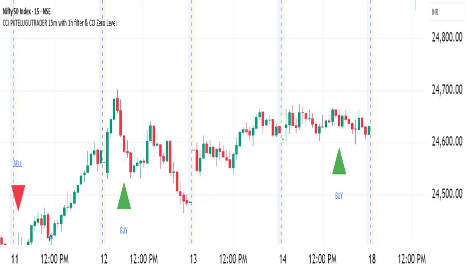
RRG Relative Strength# RRG Relative Strength (RRG RS)
Compare any symbol to a benchmark using two RRG-style lines: **RS-Ratio** (trend of relative strength) and **RS-Momentum** (momentum of that trend). Both are centered at **100**:
- **RS-Ratio > 100** → outperforming the benchmark
- **RS-Ratio < 100** → underperforming
- **RS-Momentum** often **leads** RS-Ratio (crosses 100 earlier)
# How it works
1) Relative Strength (RS): RS = Close(symbol) / Close(benchmark)
2) Normalize around 100: smooth RS with EMA and divide RS by that EMA
3) RS-Ratio: EMA( RS / EMA(RS, Length), LenSmooth ) * 100
4) RS-Momentum: RS-Ratio / EMA(RS-Ratio, LenSmooth) * 100
# Inputs
- Length (default 14): normalization window for RS
- Length Smooth (default 20): smoothing window for RS-Ratio & RS-Momentum
# Benchmark (auto)
- US: SP:SPX (S&P 500)
- Vietnam: HOSE:VNINDEX
- Crypto: INDEX:BTCUSD
(Modify the mapping if needed, or replace with your own input.symbol().)
# How to read
- Improving: RS-Momentum crosses above 100 while RS-Ratio turns up
- Leading: RS-Ratio > 100 with RS-Momentum ≥ 100
- Weakening: RS-Momentum drops below 100; RS-Ratio often follows
# Timeframes & presets
- Works on Daily and Weekly charts
- Daily (fast): 14 / 20
- Approx. weekly behavior on Daily: 50 / 60
Note: Values usually hover near 100 (e.g., ~90–110) but are not strictly bounded. Ensure your symbol and benchmark trade in comparable sessions/currencies.

Fibs Has Lied 🌟 Fibs Has Lied - Indicator Overview 🌟
Designed for indices like US30, NQ, and SPX, this indicator highlights setups where price interacts with key EMA levels during specific trading sessions (default: 6:30–11:30 AM EST).
🌟 Key Features & Levels 🌟
🔹EMA Crossover Setups
The indicator uses the 100-period and 200-period EMAs to identify bullish and bearish setups:
- Bullish Setup: Triggers when the 100 EMA crosses above the 200 EMA, followed by two consecutive candles opening above the 100 EMA, with the low within a specified point distance (e.g., 20 points for US30).
- Bearish Setup: Triggers when the 100 EMA crosses below the 200 EMA, followed by two consecutive candles opening below the 100 EMA, with the high within the point distance.
- Signals are marked with green (buy) or red (sell) triangles and text, ensuring you don’t miss a setup. 📈
🔹 Reset Conditions for Re-Entries
After an initial setup, the indicator watches for “reset” opportunities:
- Buy Reset: If price moves below the 200 EMA after a bullish crossover, then returns with two consecutive candles where lows are above the 100 EMA (within point distance), a new buy signal is plotted.
- Sell Reset: If price moves above the 200 EMA after a bearish crossover, then returns with two consecutive candles where highs are below the 100 EMA (within point distance), a new sell signal is plotted.
This feature captures additional entries after liquidity grabs or fakeouts, aligning with ICT’s manipulation concepts. 🔄
🔹 Session-Based Filtering
Focus your trades during high-liquidity windows! The default session (6:30–11:30 AM EST, New York timezone) targets the London/NY overlap, where price often seeks liquidity or sets up for reversals. Toggle the time filter off for 24/7 signals if desired. 🕒
🔹Symbol-Specific Point Distance
Customizable entry zones based on your chosen index:
- US30: 20 points from the 100 EMA.
- NQ: 3 points from the 100 EMA.
- SPX: 2.5 points from the 100 EMA.
This ensures setups are tailored to the volatility of your market, maximizing relevance. 🎯
🔹 Market Structure Markers (Optional)
Visualize swing points with pivot-based labels:
- HH (Higher High): Signals uptrend continuation.
- HL (Higher Low): Indicates potential bullish support.
- LH (Lower High): Suggests weakening uptrend or reversal.
- LL (Lower Low): Points to downtrend continuation.
- Toggle these on/off to keep your chart clean while analyzing trend direction. 📊
🔹 EMA Visualization
Optionally plot the 100 EMA (blue) and 200 EMA (red) to see key levels where price reacts. These act as dynamic support/resistance, perfect for spotting liquidity pools or ICT’s Power of 3 setups. ⚖️
🌟 Customization Options 🌟
- Symbol Selection: Choose US30, NQ, or SPX to adjust point distance for entries.
- Time Filter: Enable/disable the 6:30–11:30 AM EST session to focus on high-liquidity periods.
- EMA Display: Toggle 100/200 EMAs on/off to reduce chart clutter.
- Market Structure: Show/hide HH/HL/LH/LL labels for cleaner analysis.
- Signal Markers: Green (buy) and red (sell) triangles with text are auto-plotted for easy identification.
🌟 Usage Tips 🌟
- Best Timeframes: Use on 3m for intraday scalping and 30m for swing trades.
- Combine with ICT Tools: Pair with order blocks, fair value gaps, or kill zones for stronger setups.
- Focus on Session: The default 6:30–11:30 AM EST session captures London/NY volatility—perfect for liquidity-driven moves.
- Avoid Overcrowding: Disable market structure or EMAs if you only want setup signals.
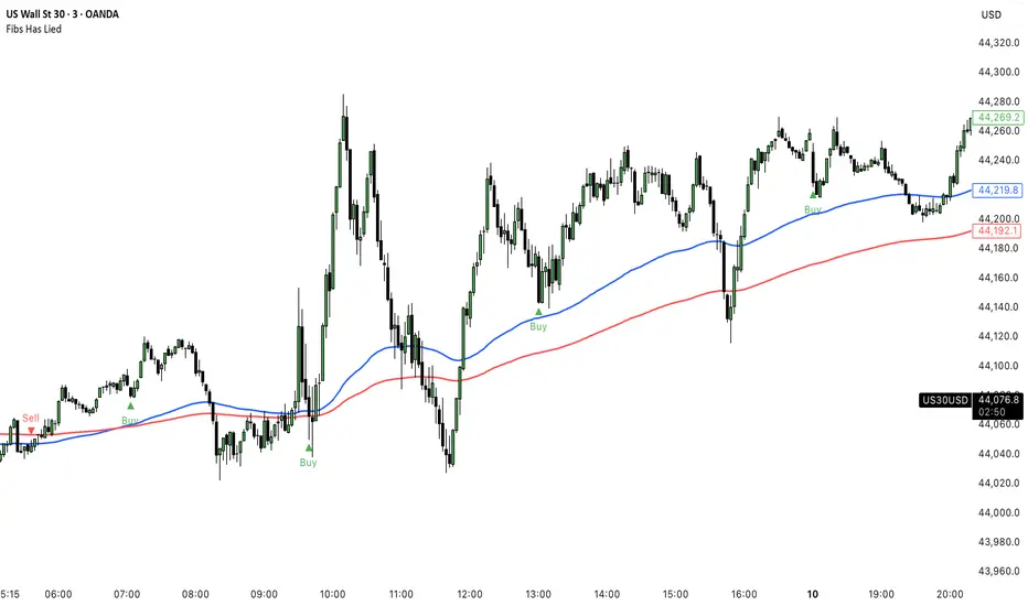
CCO_LibraryLibrary "CCO_Library"
Contrarian Crowd Oscillator (CCO) Library - Multi-oscillator consensus indicator for contrarian trading signals
@author B3AR_Trades
calculate_oscillators(rsi_length, stoch_length, cci_length, williams_length, roc_length, mfi_length, percentile_lookback, use_rsi, use_stochastic, use_williams, use_cci, use_roc, use_mfi)
Calculate normalized oscillator values
Parameters:
rsi_length (simple int) : (int) RSI calculation period
stoch_length (int) : (int) Stochastic calculation period
cci_length (int) : (int) CCI calculation period
williams_length (int) : (int) Williams %R calculation period
roc_length (int) : (int) ROC calculation period
mfi_length (int) : (int) MFI calculation period
percentile_lookback (int) : (int) Lookback period for CCI/ROC percentile ranking
use_rsi (bool) : (bool) Include RSI in calculations
use_stochastic (bool) : (bool) Include Stochastic in calculations
use_williams (bool) : (bool) Include Williams %R in calculations
use_cci (bool) : (bool) Include CCI in calculations
use_roc (bool) : (bool) Include ROC in calculations
use_mfi (bool) : (bool) Include MFI in calculations
Returns: (OscillatorValues) Normalized oscillator values
calculate_consensus_score(oscillators, use_rsi, use_stochastic, use_williams, use_cci, use_roc, use_mfi, weight_by_reliability, consensus_smoothing)
Calculate weighted consensus score
Parameters:
oscillators (OscillatorValues) : (OscillatorValues) Individual oscillator values
use_rsi (bool) : (bool) Include RSI in consensus
use_stochastic (bool) : (bool) Include Stochastic in consensus
use_williams (bool) : (bool) Include Williams %R in consensus
use_cci (bool) : (bool) Include CCI in consensus
use_roc (bool) : (bool) Include ROC in consensus
use_mfi (bool) : (bool) Include MFI in consensus
weight_by_reliability (bool) : (bool) Apply reliability-based weights
consensus_smoothing (int) : (int) Smoothing period for consensus
Returns: (float) Weighted consensus score (0-100)
calculate_consensus_strength(oscillators, consensus_score, use_rsi, use_stochastic, use_williams, use_cci, use_roc, use_mfi)
Calculate consensus strength (agreement between oscillators)
Parameters:
oscillators (OscillatorValues) : (OscillatorValues) Individual oscillator values
consensus_score (float) : (float) Current consensus score
use_rsi (bool) : (bool) Include RSI in strength calculation
use_stochastic (bool) : (bool) Include Stochastic in strength calculation
use_williams (bool) : (bool) Include Williams %R in strength calculation
use_cci (bool) : (bool) Include CCI in strength calculation
use_roc (bool) : (bool) Include ROC in strength calculation
use_mfi (bool) : (bool) Include MFI in strength calculation
Returns: (float) Consensus strength (0-100)
classify_regime(consensus_score)
Classify consensus regime
Parameters:
consensus_score (float) : (float) Current consensus score
Returns: (ConsensusRegime) Regime classification
detect_signals(consensus_score, consensus_strength, consensus_momentum, regime)
Detect trading signals
Parameters:
consensus_score (float) : (float) Current consensus score
consensus_strength (float) : (float) Current consensus strength
consensus_momentum (float) : (float) Consensus momentum
regime (ConsensusRegime) : (ConsensusRegime) Current regime classification
Returns: (TradingSignals) Trading signal conditions
calculate_cco(rsi_length, stoch_length, cci_length, williams_length, roc_length, mfi_length, consensus_smoothing, percentile_lookback, use_rsi, use_stochastic, use_williams, use_cci, use_roc, use_mfi, weight_by_reliability, detect_momentum)
Calculate complete CCO analysis
Parameters:
rsi_length (simple int) : (int) RSI calculation period
stoch_length (int) : (int) Stochastic calculation period
cci_length (int) : (int) CCI calculation period
williams_length (int) : (int) Williams %R calculation period
roc_length (int) : (int) ROC calculation period
mfi_length (int) : (int) MFI calculation period
consensus_smoothing (int) : (int) Consensus smoothing period
percentile_lookback (int) : (int) Percentile ranking lookback
use_rsi (bool) : (bool) Include RSI
use_stochastic (bool) : (bool) Include Stochastic
use_williams (bool) : (bool) Include Williams %R
use_cci (bool) : (bool) Include CCI
use_roc (bool) : (bool) Include ROC
use_mfi (bool) : (bool) Include MFI
weight_by_reliability (bool) : (bool) Apply reliability weights
detect_momentum (bool) : (bool) Calculate momentum and acceleration
Returns: (CCOResult) Complete CCO analysis results
calculate_cco_default()
Calculate CCO with default parameters
Returns: (CCOResult) CCO result with standard settings
cco_consensus_score()
Get just the consensus score with default parameters
Returns: (float) Consensus score (0-100)
cco_consensus_strength()
Get just the consensus strength with default parameters
Returns: (float) Consensus strength (0-100)
is_panic_bottom()
Check if in panic bottom condition
Returns: (bool) True if panic bottom signal active
is_euphoric_top()
Check if in euphoric top condition
Returns: (bool) True if euphoric top signal active
bullish_consensus_reversal()
Check for bullish consensus reversal
Returns: (bool) True if bullish reversal detected
bearish_consensus_reversal()
Check for bearish consensus reversal
Returns: (bool) True if bearish reversal detected
bearish_divergence()
Check for bearish divergence
Returns: (bool) True if bearish divergence detected
bullish_divergence()
Check for bullish divergence
Returns: (bool) True if bullish divergence detected
get_regime_name()
Get current regime name
Returns: (string) Current consensus regime name
get_contrarian_signal()
Get contrarian signal
Returns: (string) Current contrarian trading signal
get_position_multiplier()
Get position size multiplier
Returns: (float) Recommended position sizing multiplier
OscillatorValues
Individual oscillator values
Fields:
rsi (series float) : RSI value (0-100)
stochastic (series float) : Stochastic value (0-100)
williams (series float) : Williams %R value (0-100, normalized)
cci (series float) : CCI percentile value (0-100)
roc (series float) : ROC percentile value (0-100)
mfi (series float) : Money Flow Index value (0-100)
ConsensusRegime
Consensus regime classification
Fields:
extreme_bearish (series bool) : Extreme bearish consensus (<= 20)
moderate_bearish (series bool) : Moderate bearish consensus (20-40)
mixed (series bool) : Mixed consensus (40-60)
moderate_bullish (series bool) : Moderate bullish consensus (60-80)
extreme_bullish (series bool) : Extreme bullish consensus (>= 80)
regime_name (series string) : Text description of current regime
contrarian_signal (series string) : Contrarian trading signal
TradingSignals
Trading signals
Fields:
panic_bottom_signal (series bool) : Extreme bearish consensus with high strength
euphoric_top_signal (series bool) : Extreme bullish consensus with high strength
consensus_reversal_bullish (series bool) : Bullish consensus reversal
consensus_reversal_bearish (series bool) : Bearish consensus reversal
bearish_divergence (series bool) : Bearish price-consensus divergence
bullish_divergence (series bool) : Bullish price-consensus divergence
strong_consensus (series bool) : High consensus strength signal
CCOResult
Complete CCO calculation results
Fields:
consensus_score (series float) : Main consensus score (0-100)
consensus_strength (series float) : Consensus strength (0-100)
consensus_momentum (series float) : Rate of consensus change
consensus_acceleration (series float) : Rate of momentum change
oscillators (OscillatorValues) : Individual oscillator values
regime (ConsensusRegime) : Regime classification
signals (TradingSignals) : Trading signals
position_multiplier (series float) : Recommended position sizing multiplier

Precision Trade Zone By KittisakThis indicator is designed for Money Management calculations, helping to facilitate risk management in trading, determining suitable leverage based on acceptable risk, and adjusting the Stop Loss level to align with the calculated leverage.
Abbreviation Descriptions
LR : Suitable Leverage.
EP : Entry Price.
BEP : Break-Even Point (a point where you can move your Stop Loss to prevent losses once the price reaches a certain level).
SL : Stop Loss (a recalculated Stop Loss level to match the leverage. You should use this as the Stop Loss price instead of the initial level you set).
TP : Take Profit (a point where you take profit based on the defined risk-reward ratio).
Note
When first activating the indicator, an error may occur, and no output will be displayed. This happens because you must first specify the Entry Price and Stop Loss in the indicator settings.
How Much Leverage Should You Use?
It may seem like a simple question but is difficult to answer.
Method for Calculating Suitable Leverage
Use the formula:
Leverage = Acceptable Loss / (Distance between Entry Price and Stop Loss + (Buy Fee + Sell Fee))
Calculating the Correct Stop Loss Point
(Stop Loss levels will be slightly adjusted or extended)
For Long Positions :
New Stop Loss = Entry Price * (1 - Acceptable Loss / (Calculated Leverage * 100))
For Short Positions :
New Stop Loss = Entry Price * (1 + Acceptable Loss / (Calculated Leverage * 100))
Calculating the Correct Take Profit Point
(Take Profit levels will be slightly adjusted or extended)
For Long Positions :
Take Profit = Entry Price * (1 + (Acceptable Loss / (Calculated Leverage * 100) * RR) + ((Buy Fee + Sell Fee) / 100))
For Short Positions :
Take Profit = Entry Price * (1 - (Acceptable Loss / (Calculated Leverage * 100) * RR) + ((Buy Fee + Sell Fee) / 100))
Benefits of This Calculation
1. Accurate Risk Assessment
The calculated leverage accounts for trading fees. For example, if you aim for a 2% loss, this method ensures the actual loss is exactly 2%, not more (e.g., 2% plus fees).
2. Eliminates Guesswork
Randomly setting leverage can lead to risks because the Stop Loss level may not align with your position. This calculation ensures that the leverage aligns precisely with your desired Stop Loss level.
3. Realistic Profit Targets
For example, with a 2% acceptable loss and a 1:2 RR, you expect a 4% profit. However, without this calculation, fees may reduce your profit below 4%. This method includes fees, ensuring your profit matches the intended target.
Caution
This indicator does not account for slippage or requotes. Use it with caution and allow a buffer for slippage in your calculations.
Indicator นี้มีไว้สำหรับคำนวณ Money Management ซึ่งจะช่วยอำนวยความสะดวกในการจัดการความเสี่ยงในการเทรด การคำนวณ Leverage ที่เหมาะสมกับความเสี่ยงที่คุณยอมรับได้ และจัดการจุด Stop Loss ให้เหมาะสมกับ Leverage นั้น
คำอธิบายเกี่ยวกับคำย่อ
LR หมายถึง Leverage ที่เหมาะสม
EP หมายถึง Entry Price หรือราคาเข้าซื้อ
BEP หมายถึง Break-Even Point หรือจุดคุ้มทุน (คุณสามารถย้าย Stop Loss มาที่จุดนี้เมื่อราคาไปถึงจุดหนึ่งเพื่อป้องกันการขาดทุนได้)
SL หมายถึง Stop Loss (ซึ่งเป็น Stop Loss ที่คำนวณใหม่เพื่อให้ตำแหน่งเหมาะสมกับ Leverage ที่คำนวณได้ คุณควรใช้จุดนี้เพื่อเป็นราคา Stop Loss แทนจุด Stop Loss ที่คุณกำหนดไว้ในตอนแรก)
TP หมายถึง Take Profit (เป็นจุดที่คุณจะขายทำกำไรตาม RR ที่กำหนดไว้)
* หมายเหตุ เมื่อเริ่มเปิด Indicator จะเกิด Error ขึ้น และไม่มีผลลัพท์ใด ๆ แสดงให้เห็น นั่นเป็นเพราะคุณต้องเข้าไปกำหนด Entry Price และ Stop Loss ในการตั้งค่าของ Indicator เสียก่อน
ต้องใช้ Leverage เท่าไหร่? มันเป็นคำถามที่ดูเหมือนง่าย แต่ตอบยาก
วิธีคำนวณ Leverage ที่เหมาะสม ใช้สมการคือ
Levarage = การขาดทุนที่ยอมรับได้ / (ระยะห่างระหว่าง Entry Price และ Stop Loss + (ค่าธรรมเนียมซื้อ + ค่าธรรมเนียมขาย))
นำผลลัพท์ Leverage ที่ได้มาคำนวณเพื่อหาจุด Stop Loss ที่ถูกต้อง (จุดของ Stop Loss จะมีการยืดขยายออกไปเล็กน้อย) โดยใช้สมการ
ตำแหน่ง Stop Loss ใหม่ = Entry Price * (1 - การขาดทุนที่ยอมรับได้ / (Leverage ที่คำนวณได้ * 100)) // สำหรับ Long
ตำแหน่ง Stop Loss ใหม่ = Entry Price * (1 + การขาดทุนที่ยอมรับได้ / (Leverage ที่คำนวณได้ * 100)) // สำหรับ Short
นำผลลัพท์ Leverage ที่ได้มาคำนวณเพื่อหาจุด Take Profit ที่ถูกต้อง (จุดของ Take Profit จะมีการยืดขยายออกไปเล็กน้อย) โดยใช้สมการ
ตำแหน่ง Take Profit = Entry Price * (1 + (การขาดทุนที่ยอมรับได้ / (Leverage ที่คำนวณได้ * 100) * RR) + ((ค่าธรรมเนียมซื้อ + ค่าธรรมเนียมขาย) / 100)) // สำหรับ Long
ตำแหน่ง Take Profit = Entry Price * (1 - (การขาดทุนที่ยอมรับได้ / (Leverage ที่คำนวณได้ * 100) * RR) + ((ค่าธรรมเนียมซื้อ + ค่าธรรมเนียมขาย) / 100)) // สำหรับ Short
ข้อดีของการคำนวณคือ
1. คุณจะได้ค่า Leverage ที่เหมาะสมกับความเสี่ยงที่คุณยอมรับได้โดยรวมค่าธรรมเนียมเข้าไปในนั้นแล้ว นั่นหมายความว่า ความสูญเสียจะเป็น 2% (ตามตัวอย่าง) จริง ๆ ไม่ใช่ 2% และถูกหักค่าธรรมเนียมเพิ่มอีก กลายเป็นสูญเสียมากกว่า 2%
2. การตั้ง Leverage มั่ว ๆ กลายเป็นความเสี่ยง นั่นเพราะตำแหน่งของ Stop Loss ไม่ได้อยู่ในจุดที่ควรจะเป็น การคำนวณนี้ช่วยให้คุณได้ Leverage ในตำแหน่ง Stop Loss ที่คุณต้องการโดยแท้จริง
3. ผลกำไรที่ได้รับตรงกับความต้องการจริง ๆ เช่น การขาดทุนที่ยอมรับได้ 2% และ RR 1:2 สิ่งที่คุณคิดคือกำไร 4% แต่จริง ๆ แล้วไม่ถึง 4% นั่นเพราะว่าโดนหักค่าธรรมเนียมไปส่วนหนึ่ง การคำนวณนี้ได้รวมค่าธรรมเนียมให้แล้ว คุณจึงได้กำไรที่ 4% อย่างถูกต้องตามต้องการ
ข้อควรระวัง
Indicator นี้ไม่ได้มีการควบคุมความเสี่ยงในเรื่องของ slippage หรือ requote โปรดใช้งานอย่างระมัดระวังและมีการเผื่อระยะสำหรับ slippage ด้วย
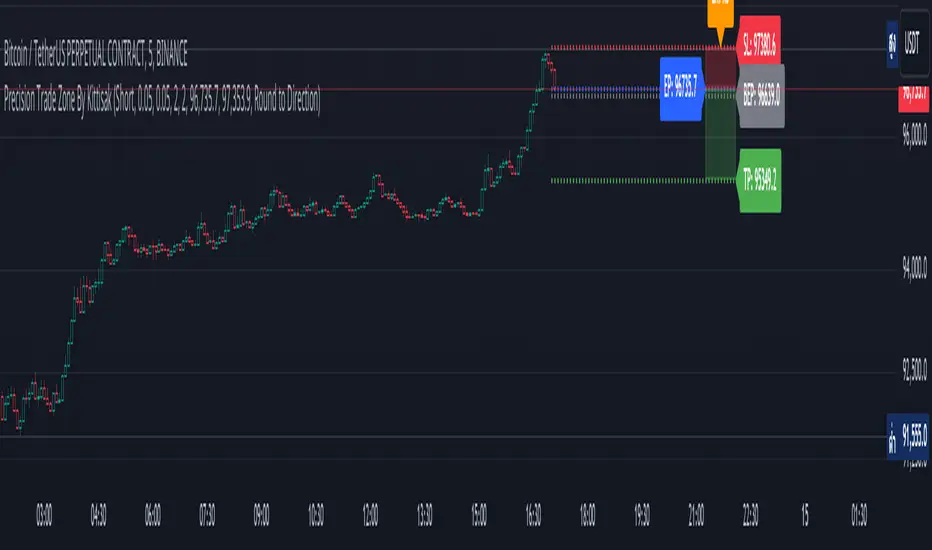
Extreme Pressure Zones Indicator (EPZ) [BullByte]Extreme Pressure Zones Indicator(EPZ)
The Extreme Pressure Zones (EPZ) Indicator is a proprietary market analysis tool designed to highlight potential overbought and oversold "pressure zones" in any financial chart. It does this by combining several unique measurements of price action and volume into a single, bounded oscillator (0–100). Unlike simple momentum or volatility indicators, EPZ captures multiple facets of market pressure: price rejection, trend momentum, supply/demand imbalance, and institutional (smart money) flow. This is not a random mashup of generic indicators; each component was chosen and weighted to reveal extreme market conditions that often precede reversals or strong continuations.
What it is?
EPZ estimates buying/selling pressure and highlights potential extreme zones with a single, bounded 0–100 oscillator built from four normalized components. Context-aware weighting adapts to volatility, trendiness, and relative volume. Visual tools include adaptive thresholds, confirmed-on-close extremes, divergence, an MTF dashboard, and optional gradient candles.
Purpose and originality (not a mashup)
Purpose: Identify when pressure is building or reaching potential extremes while filtering noise across regimes and symbols.
Originality: EPZ integrates price rejection, momentum cascade, pressure distribution, and smart money flow into one bounded scale with context-aware weighting. It is not a cosmetic mashup of public indicators.
Why a trader might use EPZ
EPZ provides a multi-dimensional gauge of market extremes that standalone indicators may miss. Traders might use it to:
Spot Reversals: When EPZ enters an "Extreme High" zone (high red), it implies selling pressure might soon dominate. This can hint at a topside reversal or at least a pause in rallies. Conversely, "Extreme Low" (green) can highlight bottom-fish opportunities. The indicator's divergence module (optional) also finds hidden bullish/bearish divergences between price and EPZ, a clue that price momentum is weakening.
Measure Momentum Shifts: Because EPZ blends momentum and volume, it reacts faster than many single metrics. A rising MPO indicates building bullish pressure, while a falling MPO shows increasing bearish pressure. Traders can use this like a refined RSI: above 50 means bullish bias, below 50 means bearish bias, but with context provided by the thresholds.
Filter Trades: In trend-following systems, one could require EPZ to be in the bullish (green) zone before taking longs, or avoid new trades when EPZ is extreme. In mean-reversion systems, one might specifically look to fade extremes flagged by EPZ.
Multi-Timeframe Confirmation: The dashboard can fetch a higher timeframe EPZ value. For example, you might trade a 15-minute chart only when the 60-minute EPZ agrees on pressure direction.
Components and how they're combined
Rejection (PRV) – Captures price rejection based on candle wicks and volume (see Price Rejection Volume).
Momentum Cascade (MCD) – Blends multiple momentum periods (3,5,8,13) into a normalized momentum score.
Pressure Distribution (PDI) – Measures net buy/sell pressure by comparing volume on up vs down candles.
Smart Money Flow (SMF) – An adaptation of money flow index that emphasizes unusual volume spikes.
Each of these components produces a 0–100 value (higher means more bullish pressure). They are then weighted and averaged into the final Market Pressure Oscillator (MPO), which is smoothed and scaled. By combining these four views, EPZ stands out as a comprehensive pressure gauge – the whole is greater than the sum of parts
Context-aware weighting:
Higher volatility → more PRV weight
Trendiness up (RSI of ATR > 25) → more MCD weight
Relative volume > 1.2x → more PDI weight
SMF holds a stable weight
The weighted average is smoothed and scaled into MPO ∈ with 50 as the neutral midline.
What makes EPZ stand out
Four orthogonal inputs (price action, momentum, pressure, flow) unified in a single bounded oscillator with consistent thresholds.
Adaptive thresholds (optional) plus robust extreme detection that also triggers on crossovers, so static thresholds work reliably too.
Confirm Extremes on Bar Close (default ON): dots/arrows/labels/alerts print on closed bars to avoid repaint confusion.
Clean dashboard, divergence tools, pre-alerts, and optional on-price gradients. Visual 3D layering uses offsets for depth only,no lookahead.
Recommended markets and timeframes
Best: liquid symbols (index futures, large-cap equities, major FX, BTC/ETH).
Timeframes: 5–15m (more signals; consider higher thresholds), 1H–4H (balanced), 1D (clear regimes).
Use caution on illiquid or very low TFs where wick/volume geometry is erratic.
Logic and thresholds
MPO ∈ ; 50 = neutral. Above 50 = bullish pressure; below 50 = bearish.
Static thresholds (defaults): thrHigh = 70, thrLow = 30; warning bands 5 pts inside extremes (65/35).
Adaptive thresholds (optional):
thrHigh = min(BaseHigh + 5, mean(MPO,100) + stdev(MPO,100) × ExtremeSensitivity)
thrLow = max(BaseLow − 5, mean(MPO,100) − stdev(MPO,100) × ExtremeSensitivity)
Extreme detection
High: MPO ≥ thrHigh with peak/slope or crossover filter.
Low: MPO ≤ thrLow with trough/slope or crossover filter.
Cooldown: 5 bars (default). A new extreme will not print until the cooldown elapses, even if MPO re-enters the zone.
Confirmation
"Confirm Extremes on Bar Close" (default ON) gates extreme markers, pre-alerts, and alerts to closed bars (non-repainting).
Divergences
Pivot-based bullish/bearish divergence; tags appear only after left/right bars elapse (lookbackPivot).
MTF
HTF MPO retrieved with lookahead_off; values can update intrabar and finalize at HTF close. This is disclosed and expected.
Inputs and defaults (key ones)
Core: Sensitivity=1.0; Analysis Period=14; Smoothing=3; Adaptive Thresholds=OFF.
Extremes: Base High=70, Base Low=30; Extreme Sensitivity=1.5; Confirm Extremes on Bar Close=ON; Cooldown=5; Dot size Small/Tiny.
Visuals: Heatmap ON; 3D depth optional; Strength bars ON; Pre-alerts OFF; Divergences ON with tags ON; Gradient candles OFF; Glow ON.
Dashboard: ON; Position=Top Right; Size=Normal; MTF ON; HTF=60m; compact overlay table on price chart.
Advanced caps: Max Oscillator Labels=80; Max Extreme Guide Lines=80; Divergence objects=60.
Dashboard: what each element means
Header: EPZ ANALYSIS.
Large readout: Current MPO; color reflects state (extreme, approaching, or neutral).
Status badge: "Extreme High/Low", "Approaching High/Low", "Bullish/Neutral/Bearish".
HTF cell (when MTF ON): Higher-timeframe MPO, color-coded vs extremes; updates intrabar, settles at HTF close.
Predicted (when MTF OFF): Simple MPO extrapolation using momentum/acceleration—illustrative only.
Thresholds: Current thrHigh/thrLow (static or adaptive).
Components: ASCII bars + values for PRV, MCD, PDI, SMF.
Market metrics: Volume Ratio (x) and ATR% of price.
Strength: Bar indicator of |MPO − 50| × 2.
Confidence: Heuristic gauge (100 in extremes, 70 in warnings, 50 with divergence, else |MPO − 50|). Convenience only, not probability.
How to read the oscillator
MPO Value (0–100): A reading of 50 is neutral. Values above ~55 are increasingly bullish (green), while below ~45 are increasingly bearish (red). Think of these as "market pressure".
Extreme Zones: When MPO climbs into the bright orange/red area (above the base-high line, default 70), the chart will display a dot and downward arrow marking that extreme. Traders often treat this as a sign to tighten stops or look for shorts. Similarly, a bright green dot/up-arrow appears when MPO falls below the base-low (30), hinting at a bullish setup.
Heatmap/Candles: If "Pressure Heatmap" is enabled, the background of the oscillator pane will fade green or red depending on MPO. Users can optionally color the price candles by MPO value (gradient candles) to see these extremes on the main chart.
Prediction Zone(optional): A dashed projection line extends the MPO forward by a small number of bars (prediction_bars) using current MPO momentum and acceleration. This is a heuristic extrapolation best used for short horizons (1–5 bars) to anticipate whether MPO may touch a warning or extreme zone. It is provisional and becomes less reliable with longer projection lengths — always confirm predicted moves with bar-close MPO and HTF context before acting.
Divergences: When price makes a higher high but EPZ makes a lower high (bearish divergence), the indicator can draw dotted lines and a "Bear Div" tag. The opposite (lower low price, higher EPZ) gives "Bull Div". These signals confirm waning momentum at extremes.
Zones: Warning bands near extremes; Extreme zones beyond thresholds.
Crossovers: MPO rising through 35 suggests easing downside pressure; falling through 65 suggests waning upside pressure.
Dots/arrows: Extreme markers appear on closed bars when confirmation is ON and respect the 5-bar cooldown.
Pre-alert dots (optional): Proximity cues in warning zones; also gated to bar close when confirmation is ON.
Histogram: Distance from neutral (50); highlights strengthening or weakening pressure.
Divergence tags: "Bear Div" = higher price high with lower MPO high; "Bull Div" = lower price low with higher MPO low.
Pressure Heatmap : Layered gradient background that visually highlights pressure strength across the MPO scale; adjustable intensity and optional zone overlays (warning / extreme) for quick visual scanning.
A typical reading: If the oscillator is rising from neutral towards the high zone (green→orange→red), the chart may see strong buying culminating in a stall. If it then turns down from the extreme, that peak EPZ dot signals sell pressure.
Alerts
EPZ: Extreme Context — fires on confirmed extremes (respects cooldown).
EPZ: Approaching Threshold — fires in warning zones if no extreme.
EPZ: Divergence — fires on confirmed pivot divergences.
Tip: Set alerts to "Once per bar close" to align with confirmation and avoid intrabar repaint.
Practical usage ideas
Trend continuation: In positive regimes (MPO > 50 and rising), pullbacks holding above 50 often precede continuation; mirror for bearish regimes.
Exhaustion caution: E High/E Low can mark exhaustion risk; many wait for MPO rollover or divergence to time fades or partial exits.
Adaptive thresholds: Useful on assets with shifting volatility regimes to maintain meaningful "extreme" levels.
MTF alignment: Prefer setups that agree with the HTF MPO to reduce countertrend noise.
Examples
Screenshots captured in TradingView Replay to freeze the bar at close so values don't fluctuate intrabar. These examples use default settings and are reproducible on the same bars; they are for illustration, not cherry-picking or performance claims.
Example 1 — BTCUSDT, 1h — E Low
MPO closed at 26.6 (below the 30 extreme), printing a confirmed E Low. HTF MPO is 26.6, so higher-timeframe pressure remains bearish. Components are subdued (Momentum/Pressure/Smart$ ≈ 29–37), with Vol Ratio ≈ 1.19x and ATR% ≈ 0.37%. A prior Bear Div flagged weakening impulse into the drop. With cooldown set to 5 bars, new extremes are rate-limited. Many traders wait for MPO to curl up and reclaim 35 or for a fresh Bull Div before considering countertrend ideas; if MPO cannot reclaim 35 and HTF stays weak, treat bounces cautiously. Educational illustration only.
Example 2 — ETHUSD, 30m — E High
A strong impulse pushed MPO into the extreme zone (≥ 70), printing a confirmed E High on close. Shortly after, MPO cooled to ~61.5 while a Bear Div appeared, showing momentum lag as price pushed a higher high. Volume and volatility were elevated (≈ 1.79x / 1.25%). With a 5-bar cooldown, additional extremes won't print immediately. Some treat E High as exhaustion risk—either waiting for MPO rollover under 65/50 to fade, or for a pullback that holds above 50 to re-join the trend if higher-timeframe pressure remains constructive. Educational illustration only.
Known limitations and caveats
The MPO line itself can change intrabar; extreme markers/alerts do not repaint when "Confirm Extremes on Bar Close" is ON.
HTF values settle at the close of the HTF bar.
Illiquid symbols or very low TFs can be noisy; consider higher thresholds or longer smoothing.
Prediction line (when enabled) is a visual extrapolation only.
For coders
Pine v6. MTF via request.security with lookahead_off.
Extremes include crossover triggers so static thresholds also yield E High/E Low.
Extreme markers and pre-alerts are gated by barstate.isconfirmed when confirmation is ON.
Arrays prune oldest objects to respect resource limits; defaults (80/80/60) are conservative for low TFs.
3D layering uses negative offsets purely for drawing depth (no lookahead).
Screenshot methodology:
To make labels legible and to demonstrate non-repainting behavior, the examples were captured in TradingView Replay with "Confirm Extremes on Bar Close" enabled. Replay is used only to freeze the bar at close so plots don't change intrabar. The examples use default settings, include both Extreme Low and Extreme High cases, and can be reproduced by scrolling to the same bars outside Replay. This is an educational illustration, not a performance claim.
Disclaimer
This script is for educational purposes only and does not constitute financial advice. Markets involve risk; past behavior does not guarantee future results. You are responsible for your own testing, risk management, and decisions.

Swing EMAWhat is Swing EMA?
Swing EMA is an exponential moving average crossover-based indicator used for low-risk directional trading.
it's used for different types of Ema 20,50,100 and 200, 3 of them are plotted on chat 20,100,200.
100 and 200 Ema is used for showing support and resistance and it contains highlights area between them and its change color according to market crossover condition.
20 moving average is used for knowing Market Behaviour and changing its color according to crossover conditions of 50 and 20 Ema.
How does it work?
It contains 4 different types of moving averages 20,50,100, 200 out of 3 are plotted on the chart.
20 Ema is used for knowing current market behavior. Its changes its color based on the crossover of 50 Ema and 20 Ema, if 20 Ema is higher than 50 Ema then it changes its color to green, and its opposites are changed their color to red when 20 Ema is lower than 50 Ema.
100 and 200 Ema used as a support and resistance and is also contain highlighted areas between them its change their color based on the crossover if 100 Ema is higher than 200 Ema a then both of them are going to change color to Green and as an opposite, if 200 Ema is higher then 100 Ema is going to change its color to red.
So in simple word 100 and 200 Ema is used as support and resistance zone and 20 Ema is used to know current market behavior.
How to use it?
It is very easy to understand by looking at the example I gave where are the two different types of phrases. phrase bull phrase and bear phrase so 100 and 200 Ema is used as a support and resistance and to tell you which phrase is currently on the market on example there is a bull phrase on the left side and bear phrase on the right side by using your technical analysis you can find out a really good spot to buy your stocks on a bull phrase and too short on the bear phrase. 20 Ema is used as a knowing the current market behavior it doesn't make any difference on buying or selling as much as 100 Ema and 200 Ema.
Tips
Don't trade against the market.
Try trade on trending stocks rather than sideways stock.
The higher the area between 100 Ema and 200 Ema is the stronger the phrase.
Do Backtesting before real trading.
Enjoy Trading.
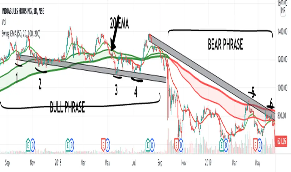
BossHouse - CCI ExtendedBossHouse - CCI Extended ( An Extended version of the Original CCI ).
The commodity channel index (CCI) is an oscillator originally introduced by Donald Lambert in 1980.
Guideline
________
Lambert's trading guidelines for the CCI focused on movements above +100 and below −100 to generate buy and sell signals. Because about 70 to 80 percent of the CCI values are between +100 and −100, a buy or sell signal will be in force only 20 to 30 percent of the time. When the CCI moves above +100, a security is considered to be entering into a strong uptrend and a buy signal is given. The position should be closed when the CCI moves back below +100. When the CCI moves below −100, the security is considered to be in a strong downtrend and a sell signal is given. The position should be closed when the CCI moves back above −100.
Since Lambert's original guidelines, traders have also found the CCI valuable for identifying reversals. The CCI is a versatile indicator capable of producing a wide array of buy and sell signals.
CCI can be used to identify overbought and oversold levels. A security would be deemed oversold when the CCI dips below −100 and overbought when it exceeds +100. From oversold levels, a buy signal might be given when the CCI moves back above −100. From overbought levels, a sell signal might be given when the CCI moved back below +100.
As with most oscillators, divergences can also be applied to increase the robustness of signals. A positive divergence below −100 would increase the robustness of a signal based on a move back above −100. A negative divergence above +100 would increase the robustness of a signal based on a move back below +100.
Trend line breaks can be used to generate signals. Trend lines can be drawn connecting the peaks and troughs. From oversold levels, an advance above −100 and trend line breakout could be considered bullish. From overbought levels, a decline below +100 and a trend line break could be considered bearish.
Settings
_______
Show 0 line
Lenght
Source
Any help and suggestions will be appreciated.
Marcos Issler @ Isslerman
marcos@bosshouse.com.br

Smart Money Flow Index (SMFI) - Advanced SMC [PhenLabs]📊Smart Money Flow Index (SMFI)
Version: PineScript™v6
📌Description
The Smart Money Flow Index (SMFI) is an advanced Smart Money Concepts implementation that tracks institutional trading behavior through multi-dimensional analysis. This comprehensive indicator combines volume-validated Order Block detection, Fair Value Gap identification with auto-mitigation tracking, dynamic Liquidity Zone mapping, and Break of Structure/Change of Character detection into a unified system.
Unlike basic SMC indicators, SMFI employs a proprietary scoring algorithm that weighs five critical factors: Order Block strength (validated by volume), Fair Value Gap size and recency, proximity to Liquidity Zones, market structure alignment (BOS/CHoCH), and multi-timeframe confluence. This produces a Smart Money Score (0-100) where readings above 70 represent optimal institutional setup conditions.
🚀Points of Innovation
Volume-Validated Order Block Detection – Only displays Order Blocks when formation candle exceeds customizable volume multiplier (default 1.5x average), filtering weak zones and highlighting true institutional accumulation/distribution
Auto-Mitigation Tracking System – Fair Value Gaps and Order Blocks automatically update status when price mitigates them, with visual distinction between active and filled zones preventing trades on dead levels
Proprietary Smart Money Score Algorithm – Combines weighted factors (OB strength 25%, FVG proximity 20%, Liquidity 20%, Structure 20%, MTF 15%) into single 0-100 confidence rating updating in real-time
ATR-Based Adaptive Calculations – All distance measurements use 14-period Average True Range ensuring consistent function across any instrument, timeframe, or volatility regime without manual recalibration
Dynamic Age Filtering – Automatically removes liquidity levels and FVGs older than configurable thresholds preventing chart clutter while maintaining relevant levels
Multi-Timeframe Confluence Integration – Analyzes higher timeframe bias with customizable multipliers (2-10x) and incorporates HTF trend direction into Smart Money Score for institutional alignment
🔧Core Components
Order Block Engine – Detects institutional supply/demand zones using characteristic patterns (down-move-then-strong-up for bullish, up-move-then-strong-down for bearish) with minimum volume threshold validation, tracks mitigation when price closes through zones
Fair Value Gap Scanner – Identifies price imbalances where current candle's low/high leaves gap with two-candle-prior high/low, filters by minimum size percentage, monitors 50% fill for mitigation status
Liquidity Zone Mapper – Uses pivot high/low detection with configurable lookback to mark swing points where stop losses cluster, extends horizontal lines to visualize sweep targets, manages lifecycle through age-based removal
Market Structure Analyzer – Tracks pivot progression to identify trend through higher-highs/higher-lows (bullish) or lower-highs/lower-lows (bearish), detects Break of Structure and Change of Character for trend/reversal confirmation
Scoring Calculation Engine – Evaluates proximity to nearest Order Blocks using ATR-normalized distance, assesses FVG recency and distance, calculates liquidity proximity with age weighting, combines structure bias and MTF trend into smoothed final score
🔥Key Features
Customizable Display Limits – Control maximum Order Blocks (1-10), Liquidity Zones (1-10), and FVG age (10-200 bars) to maintain clean charts focused on most relevant institutional levels
Gradient Strength Visualization – All zones render with transparency-adjustable coloring where stronger/newer zones appear more solid and weaker/older zones fade progressively providing instant visual hierarchy
Educational Label System – Optional labels identify each zone type (Bullish OB, Bearish OB, Bullish FVG, Bearish FVG, BOS) with color-coded text helping traders learn SMC concepts through practical application
Real-Time Smart Money Score Dashboard – Top-right table displays current score (0-100) with color coding (green >70, yellow 30-70, red <30) plus trend arrow for at-a-glance confidence assessment
Comprehensive Alert Suite – Configurable notifications for Order Block formation, Fair Value Gap detection, Break of Structure events, Change of Character signals, and high Smart Money Score readings (>70)
Buy/Sell Signal Integration – Automatically plots triangle markers when Smart Money Score exceeds 70 with aligned market structure and fresh Order Block detection providing clear entry signals
🎨Visualization
Order Block Boxes – Shaded rectangles extend from formation bar spanning high-to-low of institutional candle, bullish zones in green, bearish in red, with customizable transparency (80-98%)
Fair Value Gap Zones – Rectangular areas marking imbalances, active FVGs display in bright colors with adjustable transparency, mitigated FVGs switch to gray preventing trades on filled zones
Liquidity Level Lines – Dashed horizontal lines extend from pivot creation points, swing highs in bearish color (short targets above), swing lows in bullish color (long targets below), opacity decreases with age
Structure Labels – "BOS" labels appear above/below price when Break of Structure confirmed, colored by direction (green bullish, red bearish), positioned at 1% beyond highs/lows for visibility
Educational Info Panel – Bottom-right table explains key terminology (OB, FVG, BOS, CHoCH) and score interpretation (>70 high probability) with semi-transparent background for readability
📖Usage Guidelines
General Settings
Show Order Blocks – Default: On, toggles visibility of institutional supply/demand zones, disable when focusing solely on FVGs or Liquidity
Show Fair Value Gaps – Default: On, controls FVG zone display including active and mitigated imbalances
Show Liquidity Zones – Default: On, manages liquidity line visibility, disable on lower timeframes to reduce clutter
Show Market Structure – Default: On, toggles BOS/CHoCH label display
Show Smart Money Score – Default: On, controls score dashboard visibility
Order Block Settings
OB Lookback Period – Default: 20, Range: 5-100, controls bars scanned for Order Block patterns, lower values detect recent activity, higher values find older blocks
Min Volume Multiplier – Default: 1.5, Range: 1.0-5.0, sets minimum volume threshold as multiple of 20-period average, higher values (2.0+) filter for strongest institutional candles
Max Order Blocks to Display – Default: 3, Range: 1-10, limits simultaneous Order Blocks shown, lower settings (1-3) maintain focus on most recent zones
Fair Value Gap Settings
Min FVG Size (%) – Default: 0.3, Range: 0.1-2.0, defines minimum gap size as percentage of close price, lower values detect micro-imbalances, higher values focus on significant gaps
Max FVG Age (bars) – Default: 50, Range: 10-200, removes FVGs older than specified bars, lower settings (10-30) for scalping, higher (100-200) for swing trading
Show FVG Mitigation – Default: On, displays filled FVGs in gray providing visual history, disable to show only active untouched imbalances
Liquidity Zone Settings
Liquidity Lookback – Default: 50, Range: 20-200, sets pivot detection period for swing highs/lows, lower values (20-50) mark shorter-term liquidity, higher (100-200) identify major swings
Max Liquidity Age (bars) – Default: 100, Range: 20-500, removes liquidity lines older than specified bars, adjust based on timeframe
Liquidity Sensitivity – Default: 0.5, Range: 0.1-1.0, controls pivot detection sensitivity, lower values mark only major swings, higher values identify minor swings
Max Liquidity Zones to Display – Default: 3, Range: 1-10, limits total liquidity levels shown maintaining chart clarity
Market Structure Settings
Pivot Length – Default: 5, Range: 3-15, defines bars to left/right for pivot validation, lower values (3-5) create sensitive structure breaks, higher (10-15) filter for major shifts
Min Structure Move (%) – Default: 1.0, Range: 0.1-5.0, sets minimum percentage move required between pivots to confirm structure change
Multi-Timeframe Settings
Enable MTF Analysis – Default: On, activates higher timeframe trend analysis incorporation into Smart Money Score
Higher Timeframe Multiplier – Default: 4, Range: 2-10, multiplies current timeframe to determine analysis timeframe (4x on 15min = 1hour)
Visual Settings
Bullish Color – Default: Green (#089981), sets color for bullish Order Blocks, FVGs, and structure elements
Bearish Color – Default: Red (#f23645), defines color for bearish elements
Neutral Color – Default: Gray (#787b86), controls color of mitigated zones and neutral elements
Show Educational Labels – Default: On, displays text labels on zones identifying type (OB, FVG, BOS), disable once familiar with patterns
Order Block Transparency – Default: 92, Range: 80-98, controls Order Block box transparency
FVG Transparency – Default: 92, Range: 80-98, sets Fair Value Gap zone transparency independently from Order Blocks
Alert Settings
Alert on Order Block Formation – Default: On, triggers notification when new volume-validated Order Block detected
Alert on FVG Formation – Default: On, sends alert when Fair Value Gap appears enabling quick response to imbalances
Alert on Break of Structure – Default: On, notifies when BOS or CHoCH confirmed
Alert on High Smart Money Score – Default: On, alerts when Smart Money Score crosses above 70 threshold indicating high-probability setup
✅Best Use Cases
Order Block Retest Entries – After Break of Structure, wait for price retrace into fresh bullish Order Block with Smart Money Score >70, enter long on zone reaction targeting next liquidity level
Fair Value Gap Retracement Trading – When price creates FVG during strong move then retraces, enter as price approaches unfilled gap expecting institutional orders to continue trend
Liquidity Sweep Reversals – Monitor price approaching swing high/low liquidity zones against prevailing Smart Money Score trend, after stop hunt sweep watch for rejection into premium Order Block/FVG
Multi-Timeframe Confluence Setups – Identify alignment when current timeframe Order Block coincides with higher timeframe FVG plus MTF analysis showing matching trend bias
Break of Structure Continuations – After BOS confirms trend direction, trade pullbacks to nearest Order Block or FVG in direction of structure break using Smart Money Score >70 as entry filter
Change of Character Reversal Plays – When CHoCH detected indicating potential reversal, look for Smart Money Score pivot with opposing Order Block formation then enter on structure confirmation
⚠️Limitations
Lagging Pivot Calculations – Pivot-based features (Liquidity Zones, Market Structure) require bars to right of pivot for confirmation, meaning these elements identify levels retrospectively with delay equal to lookback period
Whipsaw in Ranging Markets – During choppy conditions, Order Blocks fail frequently and structure breaks produce false signals as Smart Money Score fluctuates without clear institutional bias, best used in trending markets
Volume Data Dependency – Order Block volume validation requires accurate volume data which may be incomplete on Forex pairs or limited in crypto exchange feeds
Subjectivity in Scoring Weights – Proprietary 25-20-20-20-15 weighting reflects general institutional behavior but may not optimize for specific instruments or market regimes, user cannot adjust factor weights
Visual Complexity on Lower Timeframes – Sub-hour timeframes generate excessive zones creating cluttered charts, requires aggressive display limit reduction and higher minimum thresholds
No Fundamental Integration – Indicator analyzes purely technical price action and volume without incorporating economic events, news catalysts, or fundamental shifts that override technical levels
💡What Makes This Unique
Unified SMC Ecosystem – Unlike indicators displaying Order Blocks OR FVGs OR Liquidity separately, SMFI combines all three institutional concepts plus market structure into single cohesive system
Proprietary Confidence Scoring – Rather than manual setup assessment, automated Smart Money Score quantifies probability by weighting five institutional dimensions into actionable 0-100 rating
Volume-Filtered Quality – Eliminates weak Order Blocks forming without institutional volume confirmation, ensuring displayed zones represent genuine accumulation/distribution
Adaptive Lifecycle Management – Automatically updates mitigation status and removes aged zones preventing trades on dead levels through continuous validity and age monitoring
Educational Integration – Built-in tooltips, labeled zones, and reference panel make indicator functional for both learning Smart Money Concepts and executing strategies
🔬How It Works
Order Block Detection – Scans for patterns where strong directional move follows counter-move creating last down-candle before rally (bullish OB) or last up-candle before sell-off (bearish OB), validates formations only when candle exhibits volume exceeding configurable multiple (default 1.5x) of 20-bar average volume
Fair Value Gap Identification – Compares current candle’s high/low against two-candles-prior low/high to detect price imbalances, calculates gap size as percentage of close and filters micro-gaps below minimum threshold (default 0.3%), monitors whether subsequent price fills 50% triggering mitigation status
Liquidity Zone Mapping – Employs pivot detection using configurable lookback (default 50 bars) to identify swing highs/lows where retail stops cluster, extends horizontal reference lines from pivot creation and applies age-based filtering to remove stale zones
Market Structure Analysis – Tracks pivot progression using structure-specific lookback (default 5 bars) to determine trend, confirms uptrend when new pivot high exceeds previous by minimum move percentage, detects Break of Structure when price breaks recent pivot level, flags Change of Character for potential reversals
Multi-Timeframe Confluence – When enabled, requests security data from higher timeframe (current TF × HTF multiplier, default 4x), compares HTF close against HTF 20-period MA to determine bias, contributes ±50 points to score ensuring alignment with institutional positioning on superior timeframe
Smart Money Score Calculation – Evaluates Order Block component via ATR-normalized distance producing max 100-point contribution weighted at 25%, assesses FVG factor through age penalty and distance at 20% weight, calculates Liquidity proximity at 20%, incorporates structure bias (±50-100 points) at 20%, adds MTF component at 15%, applies 3-period smoothing to reduce volatility
Visual Rendering and Lifecycle – Draws Order Block boxes, Fair Value Gap rectangles with color coding (green/red active, gray mitigated), extends liquidity dashed lines with fade-by-age opacity, plots BOS labels, displays Smart Money Score dashboard, continuously updates checking mitigation conditions and removing elements exceeding age/display limits
💡Note:
The Smart Money Flow Index combines multiple Smart Money Concepts into unified institutional order flow analysis. For optimal results, use the Smart Money Score as confluence filter rather than standalone entry signal – scores above 70 indicate high-probability setups but should be combined with risk management, higher timeframe bias, and market regime understanding.
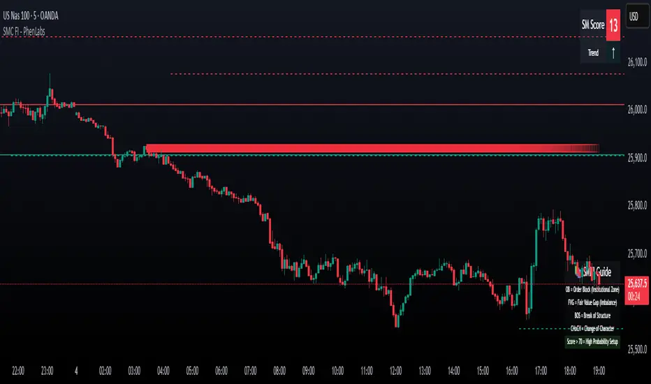
LA - Opening Price based Previous day Range PivotThis "LA - Opening Price based Previous day Range Pivot" indicator is a custom technical analysis tool designed for Trading View charts. It plots support and resistance levels (often referred to as pivots or ranges) based on the current opening price combined with the previous period's trading range. The "previous period" can be daily, weekly, or monthly, making it a multi-timeframe tool. These levels are projected using Fibonacci-inspired multipliers to create potential breakout or reversal zones.
The core idea is inspired by concepts like the Opening Range Breakout (ORB) strategy or Fibonacci pivots, but it's customized here to use a dynamic range calculation (the maximum of several absolute price differences) rather than a simple high-low range. This makes it more robust for volatile markets. Levels are symmetric above (resistance) and below (support) the opening price, helping traders identify potential entry/exit points, stop-losses, or targets. This will be useful when there is a gap-up/down as in Nifty/Sensex .
Purpose of the Indicator:
To visualize potential support/resistance zones for the current trading session based on the opening price and historical range data. This helps traders anticipate price movements, such as breakouts above resistance or bounces off support
Use Cases:
Intraday Trading: On lower timeframes (e.g., 5-min or 15-min charts), it shows daily levels for short-term trades.
Swing Trading: On higher timeframes (e.g., hourly or daily), it displays weekly/monthly levels for longer holds.
Range Identification: The filled bands highlight "zones" where price might consolidate or reverse.
Conditional Display: Levels only appear on appropriate timeframes (e.g., daily levels on intraday charts <60min), preventing clutter.
Theoretical Basis: It builds on pivot point theory, where the opening price acts as a central pivot. Multipliers (e.g., 0.618 for Fibonacci golden ratio) project levels, assuming price often respects these ratios due to market psychology.
How Calculations Work
Let's dive into the math with examples. Assume a stock with:
Current daily open (cdo) = $100
Previous daily high (pdh) = $105, low (pdl) = $95, close (pdc) = $102, close 2 days ago (pdc2) = $98
Step 1: Dynamic Range Calculation (var_d2):
This is the max of:
|pdh - pdc2| = |105 - 98| = 7
|pdl - pdc2| = |95 - 98| = 3
|pdh - pdl| = |105 - 95| = 10 (previous day range)
|pdh - cdo| = |105 - 100| = 5
|pdl - cdo| = |95 - 100| = 5
|pdc - cdo| = |102 - 100| = 2
|pdc2 - cdo| = |98 - 100| = 2
Max = 10 (so range = 10). This ensures the range accounts for gaps and extended moves, not just high-low.
Step 2: Level Projections:
Resistance (above open): Open + (Range * Multiplier)
dre6 = 100 + (10 * 1.5) = 115
dre5 = 100 + (10 * 1.27) ≈ 112.7
... down to dre0 = 100 + (10 * 0.1) = 101
dre50 = 100 + (10 * 0.5) = 105 (midpoint)
Support (below open): Open - (Range * Multiplier)
dsu0 = 100 - (10 * 0.1) = 99
... up to dsu6 = 100 - (10 * 1.5) = 85
Without Indicator
With Indicator
Pros and Cons
Pros:
Multi-Timeframe Flexibility: Seamlessly integrates daily, weekly, and monthly levels, useful for aligning short-term trades with longer trends (e.g., intraday breakout confirmed by weekly support).
Dynamic Range Calculation: Unlike standard pivots (just (H+L+C)/3), it uses max of multiple diffs, capturing gaps/volatility better—great for stocks with overnight moves.
Customizable via Inputs: Users can toggle levels, adjust multipliers, or change timeframes without editing code. Inline inputs keep the UI clean.
Visual Aids: Filled bands make zones obvious; conditional colors highlight "tight" vs. "wide" ranges (e.g., for volatility assessment).
Fibonacci Integration: Levels based on proven ratios, appealing to technical traders. Symmetric supports/resistances simplify strategy building (e.g., buy at support, sell at resistance).
No Repainting: Uses historical data with lookahead, so levels are fixed once calculated—reliable for back-testing.
Cons:
Chart Clutter: With all toggles on, 50+ plots/fills can overwhelm the chart, especially on mobile or small screens. Requires manual disabling.
Complexity for Beginners: Many inputs and calculations; without understanding fib ratios or range logic, it might confuse new users.
Performance Overhead: On low timeframes (e.g., 1-min), fetching higher TF data multiple times could lag, especially with many symbols or back-tests.
Assumes Volatility Persistence: Relies on previous range projecting future moves; in low-vol markets (e.g., sideways trends), levels may be irrelevant or too wide/narrow.
No Alerts or Signals: Purely visual; no built-in buy/sell alerts or crossover conditions—users must add separately.
Hardcoded Styles/Colors: Limited customization without code edits (e.g., can't change line styles via inputs).
Also, not optimized for non-stock assets (e.g., forex with 24/7 trading).
In summary, this is a versatile pivot tool for range-based trading based on Opening price, excelling in volatile markets but requiring some setup. If you're using it, start with defaults on a daily chart and toggle off unnecessary levels.
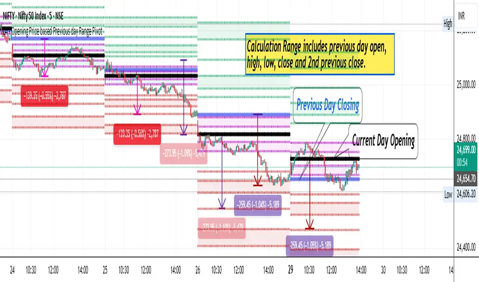
Guitar Hero [theUltimator5]The Guitar Hero indicator transforms traditional oscillator signals into a visually engaging, game-like display reminiscent of the popular Guitar Hero video game. Instead of standard line plots, this indicator presents oscillator values as colored segments or blocks, making it easier to quickly identify market conditions at a glance.
Choose from 8 different technical oscillators:
RSI (Relative Strength Index)
Stochastic %K
Stochastic %D
Williams %R
CCI (Commodity Channel Index)
MFI (Money Flow Index)
TSI (True Strength Index)
Ultimate Oscillator
Visual Display Modes
1) Boxes Mode : Creates distinct rectangular boxes for each bar, providing a clean, segmented appearance. (default)
This visual display is limited by the amount of box plots that TradingView allows on each indictor, so it will only plot a limited history. If you want to view a similar visual display that has minor breaks between boxes, then use the fill mode.
2) Fill Mode : Uses filled areas between plot boundaries.
Use this mode when you want to view the plots further back in history without the strict drawing limitations.
Five-Level Color-Coded System
The indicator normalizes all oscillator values to a 0-100 scale and categorizes them into five distinct levels:
Level 1 (Red): Very Oversold (0-19)
Level 2 (Orange): Oversold (20-29)
Level 3 (Yellow): Neutral (30-70)
Level 4 (Aqua): Overbought (71-80)
Level 5 (Lime): Very Overbought (81-100)
Customization Options
Signal Parameters
Signal Length: Primary period for oscillator calculation (default: 14)
Signal Length 2: Secondary period for Stochastic %D and TSI (default: 3)
Signal Length 3: Tertiary period for TSI calculation (default: 25)
Display Controls
Show Horizontal Reference Lines: Toggle grid lines for better level identification
Show Information Table: Display current signal type, value, and normalized value
Table Position: Choose from 9 different screen positions for the info table
Display Mode: Switch between Boxes and Fills visualization
Max Bars to Display: Control how many historical bars to show (50-450 range)
Normalization Process
The indicator automatically normalizes different oscillator ranges to a consistent 0-100 scale:
Williams %R: Converts from -100/0 range to 0-100
CCI: Maps typical -300/+300 range to 0-100
TSI: Transforms -100/+100 range to 0-100
Other oscillators: Already use 0-100 scale (RSI, Stochastic, MFI, Ultimate Oscillator)
This was designed as an educational tool
The gamified approach makes learning about oscillators more engaging for new traders.
