Gherkinit Futures Cycle█ OVERVIEW
Presented here is code for the " NYSE:GME Futures cycle theory" originally conceived by Gherkinit (Pi-Fi) and his quantitative analysts which is still under peer review.
This theory was built upon the knowledge that many intelligent investors on Reddit accrued over the past year in regards to the Mother Of All Short Squeezes this stock has to offer.
Up until now, what happened in January 2021 was considered an anomaly brought on by FOMO and retail interest but it's starting to look like unfair market makers and similar went to cover and ran head on into retail FOMO which is why they cut off the buying at that time. In order to understand what happened and what's to come, visualizing the theory with ease is essential.
█ WHAT THE SETTINGS MEAN
- Enable Draw | Visual Clean up
(True/False) Quarterly dates : Enables or disables the quarterly dates that repeat every "cycle".
(True/False) Roll dates : Enables or disables the roll dates that repeat every "cycle".
(True/False) Expiration dates : Enables or disables the expiration dates that repeat every "cycle".
(True/False) Run dates : Enables or disables the run dates that repeat every "cycle".
- Date Colors | Making things look good
(Color) Quarterly : Color for the respective date.
(Color) Roll : Color for the respective date.
(Color) Expiration : Color for the respective date.
(Color) Run : Color for the respective date.
- Extended Cycle | Look into the future
(Integer) Extended line height multiplier : A multiplier value for the height of the lines representing the selected "future" cycle.
(Dollar Amount) Extended line height : The height value in dollars of the lines representing the selected "future" cycle.
(Integer) Extended line width : The width of the lines representing the selected "future" cycle.
(Integer) Extended cycle ID : The cycle you want to see "ahead" or in the "future". For example if you set the value to "0" you'll only see cycles from the past up until the present (already occurred). If you set the value to "1" you will see the estimated dates for the specific cycle in the future i.e. 1 cycle ahead of the last completed/visible cycle on the chart.
█ EXTRA INFO
This indicator was simply made by a bored CS student who didn't want to endlessly mark dates on a graph after learning more about the theory.
Hope this help whoever uses this. To the moon fellow apes!
- Winter ;)
P.s. Pickle 4 Life
Поиск скриптов по запросу "Futures"

True Strength Index Histogram [Futures Market]This is a modified version of True Strength Index to fit the scalping trading style in futures market

Target Price for KuCoin FuturesWhen trading on KuCoin, it can be difficult to determine what you're exit price should be.
This script solves this issue by giving you an exit price based on a given entry price, a base margin, and a target profit %.
USE CASES:
No Entry Price:
If you have no position in KuCoin, then this use case could be more helpful. With no entry price inputted, two lines will be drawn above and below the current closing price.
The blue line represents your exit price for if you were to enter into a long at the current close.
The orange line represents your exit price if you were to enter into a short at the current close.
With Entry Price:
If you're already in a position in KuCoin, then this case might be more helpful.
The green line represents your exit price for a long from your entry price
The red line represents your exit price for a short from your entry price
The yellow line represents your entry price itself.

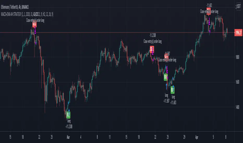
MACD oscillator with EMA strategy 4H This is a simple, yet efficient strategy, which is made from a combination of an oscillator and a moving average.
Its setup for 4h candles with the current settings, however it can be adapted to other different timeframes.
It works nicely ,beating the buy and hold for both BTC and ETH over the last 3 years.
As well with some optimizations and modifications it can be adapted to futures market, indexes(NASDAQ,NIFTY etc), forex(GBPUSD), stocks and so on.
Components:
MACD
EMA
Time condition
Long/short option
For long/exit short we enter when we are above the ema, histogram is positive and current candle is higher than previous.
For short /exit long , when close below ema, histo negative and current candles smaller than previous
If you have any questions please let me know !
Trend Surfers - Premium Breakout + AlertsTrend Surfers - Premium Breakout Strategy with Alerts
I am happy today to release the first free Trend Surfers complete Breakout Strategy!
The strategy includes:
Entry for Long and Short
Stoploss
Position Size
Exit Signal
Risk Management Feature
How the strategy works
This is a Trend Following strategy. The strategy will have drawdowns, but they will be way smaller than what you would go through with buy and old.
As a Trend Following strategy, we will buy on strength, when a breakout occurs. And sell on weakness.
The strategy includes a FIX Stoploss determined by an ATR multiple and a trailing Stoploss/Takeprofit also determined by an ATR multiple.
You can also manage your risk by entering the maximum % you are willing to risk on every trade. Additionally, there is an option to enter how many pairs you will be trading with the strategy. This will change your position size in order to make sure that you have enough funds to trade all your favorite pairs.
Use the strategy with alerts
This strategy is alert-ready. All you have to do is:
Go on a pair you would like to trade
Create an alert
Select the strategy as a Trigger
Wait for new orders to be sent to you
Every Entry (Long/Short) will include:
Market Entry (Enter position NOW!)
Stoploss price
Position Size
Leverage
* If you do not wish to use leverage, you can multiply the Position Size by the Leverage. But doing that, you might end up with a position greater than your equity. Trading on Futures is better in order to have accurate risk management.
Exit signals:
When you receive an exit signal, you need to close the position ASAP. If you want to keep your results as close as possible to the backtest results, you need to execute quickly and follow what the strategy is telling you.
Do not try to outsmart the strategy
Leave your emotion out of trading! If you trust the strategy, you will have way better returns than if you try to outsmart it. Follow each signal you receive even if it doesn't seem logical at the moment.
Become a machine that executes. Don't look at fundamentals. Follow the trend! Trust the strategy!
I hope you enjoy it!

MS POIVThis indicator was introduced by Larry Williams in 2007 and is very similar to the well known OBV indicator.
As such, it should be examined for convergence and divergence with the price trend. The interpretation can be done using the Wyckoff principles.
* Price rises, POIV stays behind => no subsequent demand
* Price meets resistance, POIV reaches new highs => supply (distribution) in the background
* Price and POIV rise synchronously => price trend is intact
These statements can of course be applied correspondingly to falling prices.
Larry Williams wrote for explanation:
Despite the problem, volume indictors have proven their worth, but while it is
a good idea to watch the cumulative flow of buying and selling pressure, you
should not assign all of this buying and selling to bulls and bears. Combined
with other concepts, such as keying off the open, we can focus on something
more germane to trading based just on volume, or what some might consider
related volatility indicators, such as daily ranges.
Futures traders can consider at least one solution to this problem: open
interest. Open interest is the number of outstanding contracts in a particular
market. (...))
The formula is calculating the cumulative sum of open interest times the net
change in price, divided by the true range. We then add the OBV value to this
cumulative sum.
So we first take the net change in price (today’s close minus yesterday’s close)
to get a percentage of where within the range the close was. Not all of the
activity will be buying or selling; the market “tells” us what percentage of
open interest goes to the buy or sell side.
Not only that, it also means we are incorporating price and trend change into
the formula.
(...)
One note of warning is necessary. The Williams POIV AD is a specific formula
that compensates for the close within the range relationship, as well telling
us how much OI to use, but it is an indicator, not a trading system. In
practice, it is useful to confirm a trade or to focus attention on a potential
trade. It is not intended to stand as the sole reason to initiate a position
in the market.

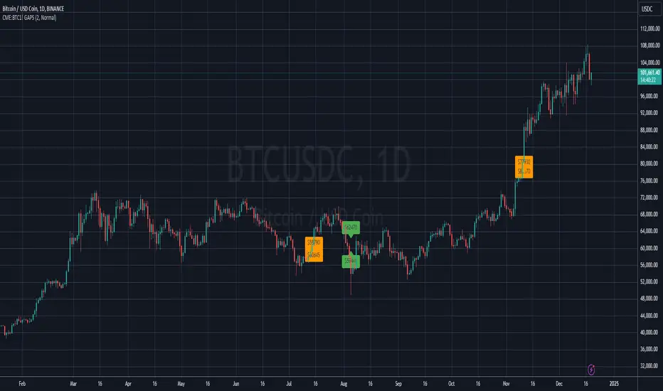
BITCOIN CME FUTURES GAPSDisplays information about Bitcoin CME Futures Gaps over BTCUSD (or XBTUSD) charts.
You can configure a threshold percentage to only display gaps whose size is greater than that percentage. The gap precentage is calculated based on the current close price.
Gaps up are displayed in Orange, gaps down in Green
MavilimW Strategy MTF EMA with HA CandlesThis is a strategy adapted initially for Mavilim moving average indicator, based on WMA MA.
It seems to works amazingly on long term markets, like stocks, some futures, some comodities and so on.
In this strategy, I form initially the candle, using EMA values, so I take the EMA of last 50 closes, open, highs and lows and form the candle
After this I take interally HA and convert the EMA candle to HA.
Then using the moving averages on multiple timeframes, like in this example we have a chart on 4h, but I use 1h and 1d moving averages.
For long condition we have : close is above moving average timeframe1 and oving average timeframe2 and oving average timeframe3
Initially short would be close below ma timeframe1, ma timeframe2 and timeframe3 -> but here I also convert it into a long signal.
So we actually go only long .
And we have 2 different exits : for first long if we have a crossdown of 1h ma with 1 day ma, and for second long if we have a cross up of 1h ma with 1 day ma in this example.
Message me if you have any questions about this strategy.

Background to highlight cash/session range [Futures]A simple script which allows the user to highlight the background of a certain session. At the moment there is only one session available, I will work on multiple highlights for numerous sessions at a later date.

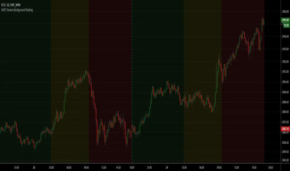
NSDT Session Background ShadingA simple script to add background colors to specific timeframes. Great for trading futures so you can separate sessions for easier viewing. Use for stocks to separate pre, open, and post market times.
There are three timeframes that can be set and all colors can be modified.
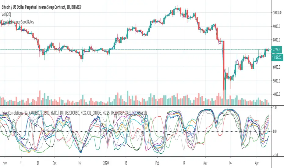
Price CorrelationsThis indicator shows price correlations of your current chart to various well-known indices.
Values above 0 mean a positive correlation, below 0 a negative correlation (not correlated).
It works well with daily candle charts and above, but you may also try it on 1h candles.
The default indices:
- Gold
- S&p 500
- Mini Dow Jones
- Dow Jones
- Russel 2000
- Nasdaq 100
- Crude Oil
- Nikkei 225 (Japan)
- FTSE 100 (UK)
- Silver
- DAX Futures (DE)
You can change the defaults to compare prices with other indices or stocks.
Bitcoin future premiumsThis shows the actual premium or the deviation between chosen active bitcoin futures and the bitcoin perpetual price as a representation of the underlying bitcoin price.
It's centered around zero meaning the futureprice and the perpetual contract are the same.
This simple indicator can for example be used to indentify sentiment in the market.
Please make sure you fill out active contracts in the settings for this indicator to work.
XBT % ContangoSimilar to my other indicators, but measures XBTUSD Contango in terms of percent.
Also, built it so you could change the values that give the red and green signals. Default values are 0% or less (backwardation) indicates green. However, i found that a 0.5% setting worked will finding local bottoms for current contract of XBTH20 (March 2020). The upper value default is at 5%, and signals red when the next contract reaches over 5%.
My assumption is as BTC increases in value over time, measuring contango in terms of percent will be a better measure of the XBT futures curve.

CME Equity Futures Price Limits
Breakers for CME's futures contracts. Should work on CST/EST/UTC charts.
CME says it uses the last 30 seconds of the session to grab a reference price, so I took the open of the last session's candle because it's easier.
Out of session breakers: +/-5%
Limit downs: -7%/-13%/-20%
There are some minor nuances for the later part of the NY session but I don't really care to add that in right now.
Options:
- Input a manual reference price to override the selected price for accuracy.
- Show only the current/last session's limits. This breaks the in session limit down lines.
Live prices:
www.cmegroup.com
Month codes:
www.cmegroup.com
Reference:
www.cmegroup.com
It's best to check the last updated reference price to ensure it's correct.


Syminfo.TypeHello traders
Earlier this week I discovered a new built-in variable called syminfo.type
What is it for?
This variable returns the type of the current symbol. Possible values are cfd, stock, futures, indices, forex, crypto, fund.
Cool bro but... should we care?
Well... we all should. Imagine you have a generic script and you want a different configuration whether you're trading FOREX or Crypto .
I designed a dummy example in that script that will preset the inputs according to the asset type from the chart.
Here I want 12/26/9 for forex and 20/50/50 for crypto - 30/60/90 otherwise
Quick caveat
It seems that for any crypto asset, syminfo.type returns "bitcoin". TradingView will fix it at some point but wanted to give you the heads-up regardless
Enjoy and all the BEST ^^
--
Dave

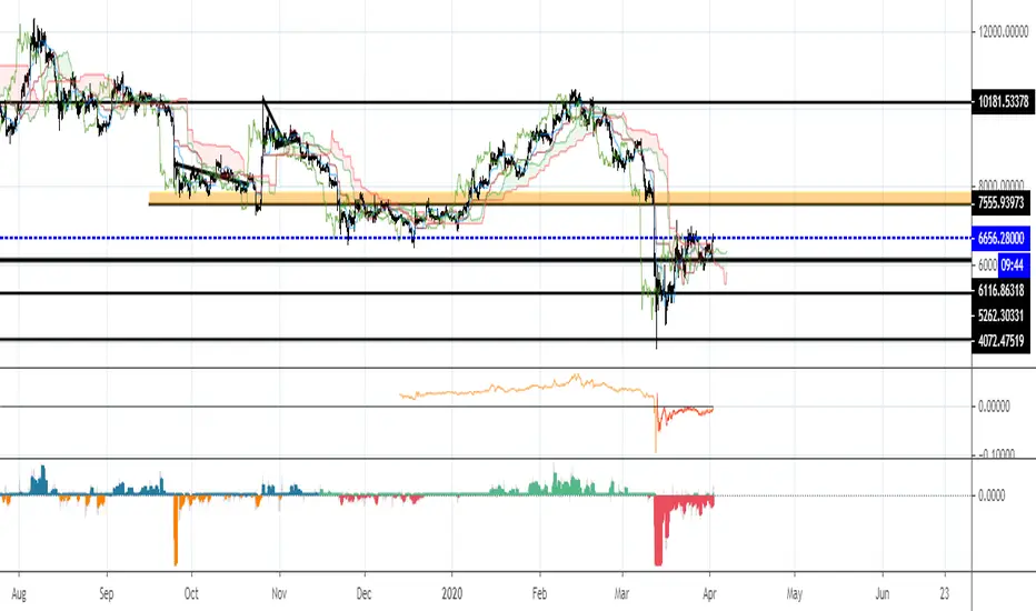
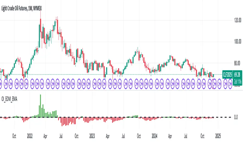
Open Interest Exponential Ease of MovementModified Ease of Movement :
* Open Interests used on Futures instead of Volume (Includes Bitcoin)
* Exponential Moving Average used instead of Simple Moving Average
* Division Number cancelled. (Division Number gives wrong signals inside strong trends.)
NOTE : This code is open source under the MIT License. If you have any improvements or corrections to suggest, please send me a pull request via the github repository github.com
Stay tuned. Best regards !
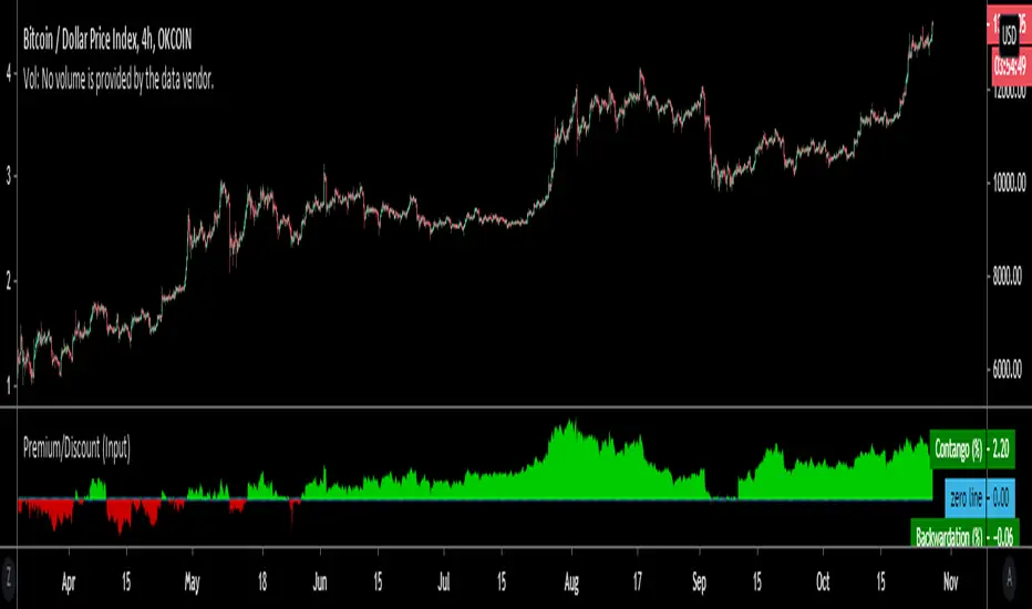
Premium/Discount (Input)Used to show Contango or Backwardation in futures contracts vs spot price. You can input your own tickers so can technically can be used to compare anything.
* In this example I'm showing Okex Quarterly contract vs Okex spot index price because it showcases it better.
* If you are using this after 2019 the default setting will not work because I set it to Bitmex which does not currently have a "current contract in front" ticker available.
It should be fairly self explanatory, but just ask below if you have any questions.
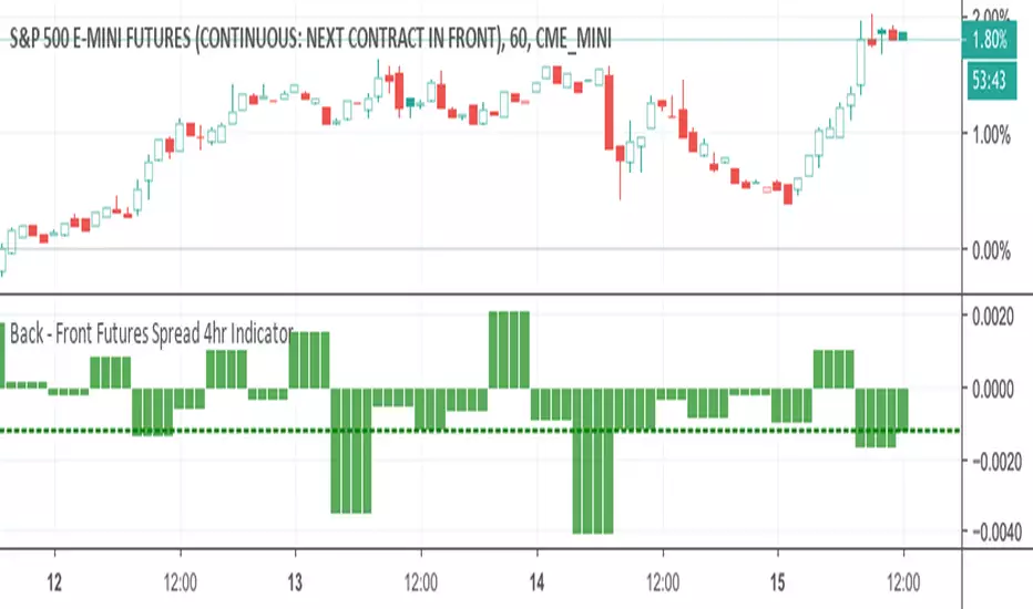
Back - Front Futures Spread 4hr IndicatorThis puts a normalized back - front spread based on the close price.
BTC Price Spread - Coinbase & Futs - Premiums & DiscountsThis indicator takes the price of Bitcoin on Coinbase and the futures price on Mex, and compares it the average price of Bitcoin across other major exchanges.
This essentials give us a spread at which Bitcoin is going for.
In turn, this could be a possible tool to help determine market sentiment.
This indicator was created for experimental purposes.
Use at your own digression.

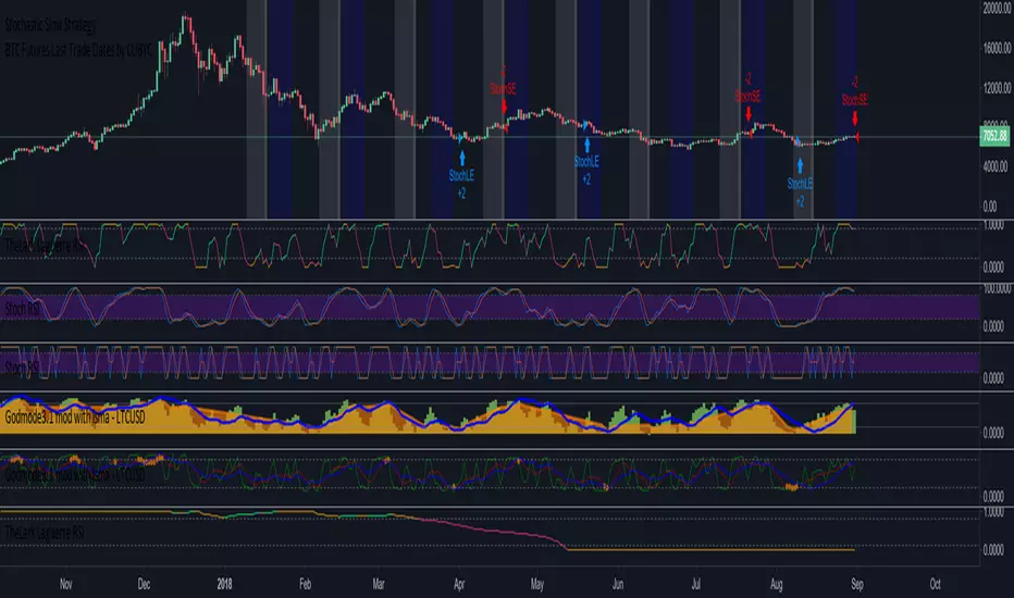
BTC Futures Settlement DatesShows the CBOE and CME settlement dates as horizontal lines, with the option to show a 7 day warning in the background. This should hopefully give ample warning.
I intend to update the script as new dates become available but please PM if I've forgotten.
