mysourcetypesncsLibrary "mysourcetypes"
Libreria personale per sorgenti estese (Close, Open, High, Low, Median, Typical, Weighted, Average, Average Median Body, Trend Biased, Trend Biased Extreme, Volume Body, Momentum Biased, Volatility Adjusted, Body Dominance, Shadow Biased, Gap Aware, Rejection Biased, Range Position, Adaptive Trend, Pressure Balanced, Impulse Wave)
rclose()
Regular Close
Returns: Close price
ropen()
Regular Open
Returns: Open price
rhigh()
Regular High
Returns: High price
rlow()
Regular Low
Returns: Low price
rmedian()
Regular Median (HL2)
Returns: (High + Low) / 2
rtypical()
Regular Typical (HLC3)
Returns: (High + Low + Close) / 3
rweighted()
Regular Weighted (HLCC4)
Returns: (High + Low + Close + Close) / 4
raverage()
Regular Average (OHLC4)
Returns: (Open + High + Low + Close) / 4
ravemedbody()
Average Median Body
Returns: (Open + Close) / 2
rtrendb()
Trend Biased Regular
Returns: Trend-weighted price
rtrendbext()
Trend Biased Extreme
Returns: Extreme trend-weighted price
rvolbody()
Volume Weighted Body
Returns: Body midpoint weighted by volume intensity
rmomentum()
Momentum Biased
Returns: Price biased towards momentum direction
rvolatility()
Volatility Adjusted
Returns: Price adjusted by candle's volatility
rbodydominance()
Body Dominance
Returns: Emphasizes body over wicks
rshadowbias()
Shadow Biased
Returns: Price biased by shadow length
rgapaware()
Gap Aware
Returns: Considers gap between candles
rrejection()
Rejection Biased
Returns: Emphasizes price rejection levels
rrangeposition()
Range Position
Returns: Where close sits within the candle range (0-100%)
radaptivetrend()
Adaptive Trend
Returns: Adapts based on recent trend strength
rpressure()
Pressure Balanced
Returns: Balances buying/selling pressure within candle
rimpulse()
Impulse Wave
Returns: Detects impulsive moves vs corrections
Поиск скриптов по запросу "OHLC"

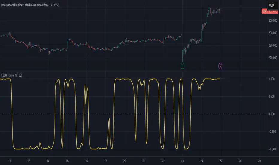
Ehlers Even Better Sinewave (EBSW)# EBSW: Ehlers Even Better Sinewave
## Overview and Purpose
The Ehlers Even Better Sinewave (EBSW) indicator, developed by John Ehlers, is an advanced cycle analysis tool. This implementation is based on a common interpretation that uses a cascade of filters: first, a High-Pass Filter (HPF) to detrend price data, followed by a Super Smoother Filter (SSF) to isolate the dominant cycle. The resulting filtered wave is then normalized using an Automatic Gain Control (AGC) mechanism, producing a bounded oscillator that fluctuates between approximately +1 and -1. It aims to provide a clear and responsive measure of market cycles.
## Core Concepts
* **Detrending (High-Pass Filter):** A 1-pole High-Pass Filter removes the longer-term trend component from the price data, allowing the indicator to focus on cyclical movements.
* **Cycle Smoothing (Super Smoother Filter):** Ehlers' Super Smoother Filter is applied to the detrended data to further refine the cycle component, offering effective smoothing with relatively low lag.
* **Wave Generation:** The output of the SSF is averaged over a short period (typically 3 bars) to create the primary "wave".
* **Automatic Gain Control (AGC):** The wave's amplitude is normalized by dividing it by the square root of its recent power (average of squared values). This keeps the oscillator bounded and responsive to changes in volatility.
* **Normalized Oscillator:** The final output is a single sinewave-like oscillator.
## Common Settings and Parameters
| Parameter | Default | Function | When to Adjust |
| ----------- | ------- | --------------------------------------------------------------------------------------------- | ----------------------------------------------------------------------------------------------------------------------------------------------- |
| Source | close | Price data used for calculation. | Typically `close`, but `hlc3` or `ohlc4` can be used for a more comprehensive price representation. |
| HP Length | 40 | Lookback period for the 1-pole High-Pass Filter used for detrending. | Shorter periods make the filter more responsive to shorter cycles; longer periods focus on longer-term cycles. Adjust based on observed cycle characteristics. |
| SSF Length | 10 | Lookback period for the Super Smoother Filter used for smoothing the detrended cycle component. | Shorter periods result in a more responsive (but potentially noisier) wave; longer periods provide more smoothing. |
**Pro Tip:** The `HP Length` and `SSF Length` parameters should be tuned based on the typical cycle lengths observed in the market and the desired responsiveness of the indicator.
## Calculation and Mathematical Foundation
**Simplified explanation:**
1. Remove the trend from the price data using a 1-pole High-Pass Filter.
2. Smooth the detrended data using a Super Smoother Filter to get a clean cycle component.
3. Average the output of the Super Smoother Filter over the last 3 bars to create a "Wave".
4. Calculate the average "Power" of the Super Smoother Filter output over the last 3 bars.
5. Normalize the "Wave" by dividing it by the square root of the "Power" to get the final EBSW value.
**Technical formula (conceptual):**
1. **High-Pass Filter (HPF - 1-pole):**
`angle_hp = 2 * PI / hpLength`
`alpha1_hp = (1 - sin(angle_hp)) / cos(angle_hp)`
`HP = (0.5 * (1 + alpha1_hp) * (src - src )) + alpha1_hp * HP `
2. **Super Smoother Filter (SSF):**
`angle_ssf = sqrt(2) * PI / ssfLength`
`alpha2_ssf = exp(-angle_ssf)`
`beta_ssf = 2 * alpha2_ssf * cos(angle_ssf)`
`c2 = beta_ssf`
`c3 = -alpha2_ssf^2`
`c1 = 1 - c2 - c3`
`Filt = c1 * (HP + HP )/2 + c2*Filt + c3*Filt `
3. **Wave Generation:**
`WaveVal = (Filt + Filt + Filt ) / 3`
4. **Power & Automatic Gain Control (AGC):**
`Pwr = (Filt^2 + Filt ^2 + Filt ^2) / 3`
`EBSW_SineWave = WaveVal / sqrt(Pwr)` (with check for Pwr == 0)
> 🔍 **Technical Note:** The combination of HPF and SSF creates a form of band-pass filter. The AGC mechanism ensures the output remains scaled, typically between -1 and +1, making it behave like a normalized oscillator.
## Interpretation Details
* **Cycle Identification:** The EBSW wave shows the current phase and strength of the dominant market cycle as filtered by the indicator. Peaks suggest cycle tops, and troughs suggest cycle bottoms.
* **Trend Reversals/Momentum Shifts:** When the EBSW wave crosses the zero line, it can indicate a potential shift in the short-term cyclical momentum.
* Crossing up through zero: Potential start of a bullish cyclical phase.
* Crossing down through zero: Potential start of a bearish cyclical phase.
* **Overbought/Oversold Levels:** While normalized, traders often establish subjective or statistically derived overbought/oversold levels (e.g., +0.85 and -0.85, or other values like +0.7, +0.9).
* Reaching above the overbought level and turning down may signal a potential cyclical peak.
* Falling below the oversold level and turning up may signal a potential cyclical trough.
## Limitations and Considerations
* **Parameter Sensitivity:** The indicator's performance depends on tuning `hpLength` and `ssfLength` to prevailing market conditions.
* **Non-Stationary Markets:** In strongly trending markets with weak cyclical components, or in very choppy non-cyclical conditions, the EBSW may produce less reliable signals.
* **Lag:** All filtering introduces some lag. The Super Smoother Filter is designed to minimize this for its degree of smoothing, but lag is still present.
* **Whipsaws:** Rapid oscillations around the zero line can occur in volatile or directionless markets.
* **Requires Confirmation:** Signals from EBSW are often best confirmed with other forms of technical analysis (e.g., price action, volume, other non-correlated indicators).
## References
* Ehlers, J. F. (2002). *Rocket Science for Traders: Digital Signal Processing Applications*. John Wiley & Sons.
* Ehlers, J. F. (2013). *Cycle Analytics for Traders: Advanced Technical Trading Concepts*. John Wiley & Sons.
Mayer Mutiple | QRMayer Multiple | QR — Publication Description
What it does
Mayer Multiple | QR is a cycle/valuation style oscillator that measures how far price sits above or below its longer-term average and normalizes that distance by current volatility. It helps you spot overheated extensions and deep discounts relative to trend, with adaptive bands that expand/contract as conditions change.
How it works (principle)
The script compares price to a long lookback moving average (default uses a 200-period average of ohlc4) and turns that gap into an oscillator.
It then computes a rolling standard deviation of that oscillator to build dynamic upper/lower bands (±1σ, ±2σ, ±3σ).
When the oscillator rises above the upper bands, the move is statistically stretched (potential distribution/risk). When it falls below the lower bands, it’s statistically depressed (potential accumulation/opportunity).
A small baseline band around zero (scaled from volatility) provides a quick trend-bias read without crowding the view.
Why this matters: Classic “Mayer Multiple” tools use a fixed threshold over a single moving average. This version is volatility-aware: its bands adapt to the market’s current dispersion, reducing false signals in quiet regimes and avoiding constant “overheat” flags in high-vol regimes.
What you see on the chart
White oscillator line: volatility-normalized deviation from the long-term average.
Adaptive bands:
Upper 1/2/3σ (shaded blue tones) = progressively more extended.
Lower 1/2/3σ (shaded green tones) = progressively more discounted.
Baseline ribbon: subtle band around zero for quick bias.
Background highlights: optional flashes when the oscillator exceeds the ±3σ extremes.
All visuals are generated by this script alone; no other indicator is required to understand usage.
How to use it
Context: Use on higher timeframes to gauge where price sits versus its long-term “fair value corridor.”
Signal reading:
Above +1σ/+2σ/+3σ: extension → consider de-risking, trailing stops, or waiting for mean reversion.
Below −1σ/−2σ/−3σ: discount → consider scaling in, watching for trend resumption cues.
Confluence: Treat it as a condition, not a trigger. Pair with structure (higher highs/lows), breadth, or momentum for entries/exits.
Regime awareness: As volatility rises, bands widen; prioritize trend context over single print extremes.
Inputs you can tune
Color mode: preset palettes for lines/fills/backgrounds.
Dynamic Threshold Length: lookback for the volatility (σ) calculation driving the adaptive bands.
Source: price input used for the long-term reference.
Band toggles: show/hide ±1σ / ±2σ / ±3σ envelopes to reduce clutter.
Originality & value
Adaptive, volatility-aware implementation of a Mayer-style concept: rather than one fixed threshold, it scales to current regime, keeping readings comparable across cycles.
Clear, clean presentation (oscillator + bands + optional background) designed for publication with a clean chart so the script’s output is immediately identifiable.
Offers actionable context (stretch/discount zones) while leaving trade execution to the user’s process.
Limitations & good practices
Best used for context and risk framing, not stand-alone entries.
Adaptive bands depend on the lookback you choose; very short windows can overfit, very long windows can lag.
Extremes can persist in strong trends—don’t fade momentum blindly.
Disclaimer
This tool is for research and education only and not investment advice. Markets involve risk. Past performance does not predict or guarantee future results. Use prudent risk management and test settings on your instruments/timeframes.

DynLenLibLibrary "DynLenLib"
sum_dyn(src, len)
Parameters:
src (float)
len (int)
lag_dyn(src, len)
Parameters:
src (float)
len (int)
highest_dyn(src, len)
Parameters:
src (float)
len (int)
lowest_dyn(src, len)
Parameters:
src (float)
len (int)
var_dyn(src, len)
Parameters:
src (float)
len (int)
stdev_dyn(src, len)
Parameters:
src (float)
len (int)
hl2()
hlc3()
ohlc4()
sma_dyn(src, len)
Parameters:
src (float)
len (int)
ema_dyn(src, len)
Parameters:
src (float)
len (int)
rma_dyn(src, len)
Parameters:
src (float)
len (int)
smma_dyn(src, len)
Parameters:
src (float)
len (int)
wma_dyn(src, len)
Parameters:
src (float)
len (int)
vwma_dyn(price, vol, len)
Parameters:
price (float)
vol (float)
len (int)
hma_dyn(src, len)
Parameters:
src (float)
len (int)
dema_dyn(src, len)
Parameters:
src (float)
len (int)
tema_dyn(src, len)
Parameters:
src (float)
len (int)
kama_dyn(src, erLen, fastLen, slowLen)
Parameters:
src (float)
erLen (int)
fastLen (int)
slowLen (int)
mcginley_dyn(src, len)
Parameters:
src (float)
len (int)
median_price()
true_range()
atr_dyn(len)
Parameters:
len (int)
bbands_dyn(src, len, mult)
Parameters:
src (float)
len (int)
mult (float)
bb_percent_b(src, len, mult)
Parameters:
src (float)
len (int)
mult (float)
bb_bandwidth(src, len, mult)
Parameters:
src (float)
len (int)
mult (float)
keltner_dyn(src, lenEMA, lenATR, multATR)
Parameters:
src (float)
lenEMA (int)
lenATR (int)
multATR (float)
donchian_dyn(len)
Parameters:
len (int)
choppiness_index(len)
Parameters:
len (int)
vol_stop(lenATR, mult)
Parameters:
lenATR (int)
mult (float)
roc_dyn(src, len)
Parameters:
src (float)
len (int)
rsi_dyn(src, len)
Parameters:
src (float)
len (int)
stoch_dyn(kLen, dLen, smoothK)
Parameters:
kLen (int)
dLen (int)
smoothK (int)
stoch_rsi_dyn(rsiLen, stochLen, kSmooth, dLen)
Parameters:
rsiLen (int)
stochLen (int)
kSmooth (int)
dLen (int)
cci_dyn(src, len)
Parameters:
src (float)
len (int)
cmo_dyn(src, len)
Parameters:
src (float)
len (int)
trix_dyn(len)
Parameters:
len (int)
tsi_dyn(shortLen, longLen)
Parameters:
shortLen (int)
longLen (int)
ultimate_osc(len1, len2, len3)
Parameters:
len1 (int)
len2 (int)
len3 (int)
dpo_dyn(src, len)
Parameters:
src (float)
len (int)
willr_dyn(len)
Parameters:
len (int)
macd_dyn(src, fastLen, slowLen, sigLen)
Parameters:
src (float)
fastLen (int)
slowLen (int)
sigLen (int)
ppo_dyn(src, fastLen, slowLen, sigLen)
Parameters:
src (float)
fastLen (int)
slowLen (int)
sigLen (int)
aroon_dyn(len)
Parameters:
len (int)
dmi_adx_dyn(diLen, adxLen)
Parameters:
diLen (int)
adxLen (int)
vortex_dyn(len)
Parameters:
len (int)
coppock_dyn(rocLen1, rocLen2, wmaLen)
Parameters:
rocLen1 (int)
rocLen2 (int)
wmaLen (int)
rvi_dyn(len)
Parameters:
len (int)
price_osc_dyn(src, fastLen, slowLen)
Parameters:
src (float)
fastLen (int)
slowLen (int)
rci_dyn(src, len)
Parameters:
src (float)
len (int)
obv()
pvt()
cmf_dyn(len)
Parameters:
len (int)
adl()
chaikin_osc_dyn(fastLen, slowLen)
Parameters:
fastLen (int)
slowLen (int)
mfi_dyn(len)
Parameters:
len (int)
volume_osc_dyn(fastLen, slowLen)
Parameters:
fastLen (int)
slowLen (int)
up_down_volume()
cvd()
supertrend_dyn(atrLen, mult)
Parameters:
atrLen (int)
mult (float)
envelopes_dyn(src, len, pct)
Parameters:
src (float)
len (int)
pct (float)
linreg_line_slope(src, len)
Parameters:
src (float)
len (int)
lsma_dyn(src, len)
Parameters:
src (float)
len (int)
corrcoef_dyn(a, b, len)
Parameters:
a (float)
b (float)
len (int)
psar(step, maxStep)
Parameters:
step (float)
maxStep (float)
pivots_standard()
williams_alligator(src, jawLen, teethLen, lipsLen)
Parameters:
src (float)
jawLen (int)
teethLen (int)
lipsLen (int)
twap_dyn(src, len)
Parameters:
src (float)
len (int)
vwap_anchored(price, volume, reset)
Parameters:
price (float)
volume (float)
reset (bool)
performance_pct(len)
Parameters:
len (int)

Keltner Channel Enhanced [DCAUT]█ Keltner Channel Enhanced
📊 ORIGINALITY & INNOVATION
The Keltner Channel Enhanced represents an important advancement over standard Keltner Channel implementations by introducing dual flexibility in moving average selection for both the middle band and ATR calculation. While traditional Keltner Channels typically use EMA for the middle band and RMA (Wilder's smoothing) for ATR, this enhanced version provides access to 25+ moving average algorithms for both components, enabling traders to fine-tune the indicator's behavior to match specific market characteristics and trading approaches.
Key Advancements:
Dual MA Algorithm Flexibility: Independent selection of moving average types for middle band (25+ options) and ATR smoothing (25+ options), allowing optimization of both trend identification and volatility measurement separately
Enhanced Trend Sensitivity: Ability to use faster algorithms (HMA, T3) for middle band while maintaining stable volatility measurement with traditional ATR smoothing, or vice versa for different trading strategies
Adaptive Volatility Measurement: Choice of ATR smoothing algorithm affects channel responsiveness to volatility changes, from highly reactive (SMA, EMA) to smoothly adaptive (RMA, TEMA)
Comprehensive Alert System: Five distinct alert conditions covering breakouts, trend changes, and volatility expansion, enabling automated monitoring without constant chart observation
Multi-Timeframe Compatibility: Works effectively across all timeframes from intraday scalping to long-term position trading, with independent optimization of trend and volatility components
This implementation addresses key limitations of standard Keltner Channels: fixed EMA/RMA combination may not suit all market conditions or trading styles. By decoupling the trend component from volatility measurement and allowing independent algorithm selection, traders can create highly customized configurations for specific instruments and market phases.
📐 MATHEMATICAL FOUNDATION
Keltner Channel Enhanced uses a three-component calculation system that combines a flexible moving average middle band with ATR-based (Average True Range) upper and lower channels, creating volatility-adjusted trend-following bands.
Core Calculation Process:
1. Middle Band (Basis) Calculation:
The basis line is calculated using the selected moving average algorithm applied to the price source over the specified period:
basis = ma(source, length, maType)
Supported algorithms include EMA (standard choice, trend-biased), SMA (balanced and symmetric), HMA (reduced lag), WMA, VWMA, TEMA, T3, KAMA, and 17+ others.
2. Average True Range (ATR) Calculation:
ATR measures market volatility by calculating the average of true ranges over the specified period:
trueRange = max(high - low, abs(high - close ), abs(low - close ))
atrValue = ma(trueRange, atrLength, atrMaType)
ATR smoothing algorithm significantly affects channel behavior, with options including RMA (standard, very smooth), SMA (moderate smoothness), EMA (fast adaptation), TEMA (smooth yet responsive), and others.
3. Channel Calculation:
Upper and lower channels are positioned at specified multiples of ATR from the basis:
upperChannel = basis + (multiplier × atrValue)
lowerChannel = basis - (multiplier × atrValue)
Standard multiplier is 2.0, providing channels that dynamically adjust width based on market volatility.
Keltner Channel vs. Bollinger Bands - Key Differences:
While both indicators create volatility-based channels, they use fundamentally different volatility measures:
Keltner Channel (ATR-based):
Uses Average True Range to measure actual price movement volatility
Incorporates gaps and limit moves through true range calculation
More stable in trending markets, less prone to extreme compression
Better reflects intraday volatility and trading range
Typically fewer band touches, making touches more significant
More suitable for trend-following strategies
Bollinger Bands (Standard Deviation-based):
Uses statistical standard deviation to measure price dispersion
Based on closing prices only, doesn't account for intraday range
Can compress significantly during consolidation (squeeze patterns)
More touches in ranging markets
Better suited for mean-reversion strategies
Provides statistical probability framework (95% within 2 standard deviations)
Algorithm Combination Effects:
The interaction between middle band MA type and ATR MA type creates different indicator characteristics:
Trend-Focused Configuration (Fast MA + Slow ATR): Middle band uses HMA/EMA/T3, ATR uses RMA/TEMA, quick trend changes with stable channel width, suitable for trend-following
Volatility-Focused Configuration (Slow MA + Fast ATR): Middle band uses SMA/WMA, ATR uses EMA/SMA, stable trend with dynamic channel width, suitable for volatility trading
Balanced Configuration (Standard EMA/RMA): Classic Keltner Channel behavior, time-tested combination, suitable for general-purpose trend following
Adaptive Configuration (KAMA + KAMA): Self-adjusting indicator responding to efficiency ratio, suitable for markets with varying trend strength and volatility regimes
📊 COMPREHENSIVE SIGNAL ANALYSIS
Keltner Channel Enhanced provides multiple signal categories optimized for trend-following and breakout strategies.
Channel Position Signals:
Upper Channel Interaction:
Price Touching Upper Channel: Strong bullish momentum, price moving more than typical volatility range suggests, potential continuation signal in established uptrends
Price Breaking Above Upper Channel: Exceptional strength, price exceeding normal volatility expectations, consider adding to long positions or tightening trailing stops
Price Riding Upper Channel: Sustained strong uptrend, characteristic of powerful bull moves, stay with trend and avoid premature profit-taking
Price Rejection at Upper Channel: Momentum exhaustion signal, consider profit-taking on longs or waiting for pullback to middle band for reentry
Lower Channel Interaction:
Price Touching Lower Channel: Strong bearish momentum, price moving more than typical volatility range suggests, potential continuation signal in established downtrends
Price Breaking Below Lower Channel: Exceptional weakness, price exceeding normal volatility expectations, consider adding to short positions or protecting against further downside
Price Riding Lower Channel: Sustained strong downtrend, characteristic of powerful bear moves, stay with trend and avoid premature covering
Price Rejection at Lower Channel: Momentum exhaustion signal, consider covering shorts or waiting for bounce to middle band for reentry
Middle Band (Basis) Signals:
Trend Direction Confirmation:
Price Above Basis: Bullish trend bias, middle band acts as dynamic support in uptrends, consider long positions or holding existing longs
Price Below Basis: Bearish trend bias, middle band acts as dynamic resistance in downtrends, consider short positions or avoiding longs
Price Crossing Above Basis: Potential trend change from bearish to bullish, early signal to establish long positions
Price Crossing Below Basis: Potential trend change from bullish to bearish, early signal to establish short positions or exit longs
Pullback Trading Strategy:
Uptrend Pullback: Price pulls back from upper channel to middle band, finds support, and resumes upward, ideal long entry point
Downtrend Bounce: Price bounces from lower channel to middle band, meets resistance, and resumes downward, ideal short entry point
Basis Test: Strong trends often show price respecting the middle band as support/resistance on pullbacks
Failed Test: Price breaking through middle band against trend direction signals potential reversal
Volatility-Based Signals:
Narrow Channels (Low Volatility):
Consolidation Phase: Channels contract during periods of reduced volatility and directionless price action
Breakout Preparation: Narrow channels often precede significant directional moves as volatility cycles
Trading Approach: Reduce position sizes, wait for breakout confirmation, avoid range-bound strategies within channels
Breakout Direction: Monitor for price breaking decisively outside channel range with expanding width
Wide Channels (High Volatility):
Trending Phase: Channels expand during strong directional moves and increased volatility
Momentum Confirmation: Wide channels confirm genuine trend with substantial volatility backing
Trading Approach: Trend-following strategies excel, wider stops necessary, mean-reversion strategies risky
Exhaustion Signs: Extreme channel width (historical highs) may signal approaching consolidation or reversal
Advanced Pattern Recognition:
Channel Walking Pattern:
Upper Channel Walk: Price consistently touches or exceeds upper channel while staying above basis, very strong uptrend signal, hold longs aggressively
Lower Channel Walk: Price consistently touches or exceeds lower channel while staying below basis, very strong downtrend signal, hold shorts aggressively
Basis Support/Resistance: During channel walks, price typically uses middle band as support/resistance on minor pullbacks
Pattern Break: Price crossing basis during channel walk signals potential trend exhaustion
Squeeze and Release Pattern:
Squeeze Phase: Channels narrow significantly, price consolidates near middle band, volatility contracts
Direction Clues: Watch for price positioning relative to basis during squeeze (above = bullish bias, below = bearish bias)
Release Trigger: Price breaking outside narrow channel range with expanding width confirms breakout
Follow-Through: Measure squeeze height and project from breakout point for initial profit targets
Channel Expansion Pattern:
Breakout Confirmation: Rapid channel widening confirms volatility increase and genuine trend establishment
Entry Timing: Enter positions early in expansion phase before trend becomes overextended
Risk Management: Use channel width to size stops appropriately, wider channels require wider stops
Basis Bounce Pattern:
Clean Bounce: Price touches middle band and immediately reverses, confirms trend strength and entry opportunity
Multiple Bounces: Repeated basis bounces indicate strong, sustainable trend
Bounce Failure: Price penetrating basis signals weakening trend and potential reversal
Divergence Analysis:
Price/Channel Divergence: Price makes new high/low while staying within channel (not reaching outer band), suggests momentum weakening
Width/Price Divergence: Price breaks to new extremes but channel width contracts, suggests move lacks conviction
Reversal Signal: Divergences often precede trend reversals or significant consolidation periods
Multi-Timeframe Analysis:
Keltner Channels work particularly well in multi-timeframe trend-following approaches:
Three-Timeframe Alignment:
Higher Timeframe (Weekly/Daily): Identify major trend direction, note price position relative to basis and channels
Intermediate Timeframe (Daily/4H): Identify pullback opportunities within higher timeframe trend
Lower Timeframe (4H/1H): Time precise entries when price touches middle band or lower channel (in uptrends) with rejection
Optimal Entry Conditions:
Best Long Entries: Higher timeframe in uptrend (price above basis), intermediate timeframe pulls back to basis, lower timeframe shows rejection at middle band or lower channel
Best Short Entries: Higher timeframe in downtrend (price below basis), intermediate timeframe bounces to basis, lower timeframe shows rejection at middle band or upper channel
Risk Management: Use higher timeframe channel width to set position sizing, stops below/above higher timeframe channels
🎯 STRATEGIC APPLICATIONS
Keltner Channel Enhanced excels in trend-following and breakout strategies across different market conditions.
Trend Following Strategy:
Setup Requirements:
Identify established trend with price consistently on one side of basis line
Wait for pullback to middle band (basis) or brief penetration through it
Confirm trend resumption with price rejection at basis and move back toward outer channel
Enter in trend direction with stop beyond basis line
Entry Rules:
Uptrend Entry:
Price pulls back from upper channel to middle band, shows support at basis (bullish candlestick, momentum divergence)
Enter long on rejection/bounce from basis with stop 1-2 ATR below basis
Aggressive: Enter on first touch; Conservative: Wait for confirmation candle
Downtrend Entry:
Price bounces from lower channel to middle band, shows resistance at basis (bearish candlestick, momentum divergence)
Enter short on rejection/reversal from basis with stop 1-2 ATR above basis
Aggressive: Enter on first touch; Conservative: Wait for confirmation candle
Trend Management:
Trailing Stop: Use basis line as dynamic trailing stop, exit if price closes beyond basis against position
Profit Taking: Take partial profits at opposite channel, move stops to basis
Position Additions: Add to winners on subsequent basis bounces if trend intact
Breakout Strategy:
Setup Requirements:
Identify consolidation period with contracting channel width
Monitor price action near middle band with reduced volatility
Wait for decisive breakout beyond channel range with expanding width
Enter in breakout direction after confirmation
Breakout Confirmation:
Price breaks clearly outside channel (upper for longs, lower for shorts), channel width begins expanding from contracted state
Volume increases significantly on breakout (if using volume analysis)
Price sustains outside channel for multiple bars without immediate reversal
Entry Approaches:
Aggressive: Enter on initial break with stop at opposite channel or basis, use smaller position size
Conservative: Wait for pullback to broken channel level, enter on rejection and resumption, tighter stop
Volatility-Based Position Sizing:
Adjust position sizing based on channel width (ATR-based volatility):
Wide Channels (High ATR): Reduce position size as stops must be wider, calculate position size using ATR-based risk calculation: Risk / (Stop Distance in ATR × ATR Value)
Narrow Channels (Low ATR): Increase position size as stops can be tighter, be cautious of impending volatility expansion
ATR-Based Risk Management: Use ATR-based risk calculations, position size = 0.01 × Capital / (2 × ATR), use multiples of ATR (1-2 ATR) for adaptive stops
Algorithm Selection Guidelines:
Different market conditions benefit from different algorithm combinations:
Strong Trending Markets: Middle band use EMA or HMA, ATR use RMA, capture trends quickly while maintaining stable channel width
Choppy/Ranging Markets: Middle band use SMA or WMA, ATR use SMA or WMA, avoid false trend signals while identifying genuine reversals
Volatile Markets: Middle band and ATR both use KAMA or FRAMA, self-adjusting to changing market conditions reduces manual optimization
Breakout Trading: Middle band use SMA, ATR use EMA or SMA, stable trend with dynamic channels highlights volatility expansion early
Scalping/Day Trading: Middle band use HMA or T3, ATR use EMA or TEMA, both components respond quickly
Position Trading: Middle band use EMA/TEMA/T3, ATR use RMA or TEMA, filter out noise for long-term trend-following
📋 DETAILED PARAMETER CONFIGURATION
Understanding and optimizing parameters is essential for adapting Keltner Channel Enhanced to specific trading approaches.
Source Parameter:
Close (Most Common): Uses closing price, reflects daily settlement, best for end-of-day analysis and position trading, standard choice
HL2 (Median Price): Smooths out closing bias, better represents full daily range in volatile markets, good for swing trading
HLC3 (Typical Price): Gives more weight to close while including full range, popular for intraday applications, slightly more responsive than HL2
OHLC4 (Average Price): Most comprehensive price representation, smoothest option, good for gap-prone markets or highly volatile instruments
Length Parameter:
Controls the lookback period for middle band (basis) calculation:
Short Periods (10-15): Very responsive to price changes, suitable for day trading and scalping, higher false signal rate
Standard Period (20 - Default): Represents approximately one month of trading, good balance between responsiveness and stability, suitable for swing and position trading
Medium Periods (30-50): Smoother trend identification, fewer false signals, better for position trading and longer holding periods
Long Periods (50+): Very smooth, identifies major trends only, minimal false signals but significant lag, suitable for long-term investment
Optimization by Timeframe: 1-15 minute charts use 10-20 period, 30-60 minute charts use 20-30 period, 4-hour to daily charts use 20-40 period, weekly charts use 20-30 weeks.
ATR Length Parameter:
Controls the lookback period for Average True Range calculation, affecting channel width:
Short ATR Periods (5-10): Very responsive to recent volatility changes, standard is 10 (Keltner's original specification), may be too reactive in whipsaw conditions
Standard ATR Period (10 - Default): Chester Keltner's original specification, good balance between responsiveness and stability, most widely used
Medium ATR Periods (14-20): Smoother channel width, ATR 14 aligns with Wilder's original ATR specification, good for position trading
Long ATR Periods (20+): Very smooth channel width, suitable for long-term trend-following
Length vs. ATR Length Relationship: Equal values (20/20) provide balanced responsiveness, longer ATR (20/14) gives more stable channel width, shorter ATR (20/10) is standard configuration, much shorter ATR (20/5) creates very dynamic channels.
Multiplier Parameter:
Controls channel width by setting ATR multiples:
Lower Values (1.0-1.5): Tighter channels with frequent price touches, more trading signals, higher false signal rate, better for range-bound and mean-reversion strategies
Standard Value (2.0 - Default): Chester Keltner's recommended setting, good balance between signal frequency and reliability, suitable for both trending and ranging strategies
Higher Values (2.5-3.0): Wider channels with less frequent touches, fewer but potentially higher-quality signals, better for strong trending markets
Market-Specific Optimization: High volatility markets (crypto, small-caps) use 2.5-3.0 multiplier, medium volatility markets (major forex, large-caps) use 2.0 multiplier, low volatility markets (bonds, utilities) use 1.5-2.0 multiplier.
MA Type Parameter (Middle Band):
Critical selection that determines trend identification characteristics:
EMA (Exponential Moving Average - Default): Standard Keltner Channel choice, Chester Keltner's original specification, emphasizes recent prices, faster response to trend changes, suitable for all timeframes
SMA (Simple Moving Average): Equal weighting of all data points, no directional bias, slower than EMA, better for ranging markets and mean-reversion
HMA (Hull Moving Average): Minimal lag with smooth output, excellent for fast trend identification, best for day trading and scalping
TEMA (Triple Exponential Moving Average): Advanced smoothing with reduced lag, responsive to trends while filtering noise, suitable for volatile markets
T3 (Tillson T3): Very smooth with minimal lag, excellent for established trend identification, suitable for position trading
KAMA (Kaufman Adaptive Moving Average): Automatically adjusts speed based on market efficiency, slow in ranging markets, fast in trends, suitable for markets with varying conditions
ATR MA Type Parameter:
Determines how Average True Range is smoothed, affecting channel width stability:
RMA (Wilder's Smoothing - Default): J. Welles Wilder's original ATR smoothing method, very smooth, slow to adapt to volatility changes, provides stable channel width
SMA (Simple Moving Average): Equal weighting, moderate smoothness, faster response to volatility changes than RMA, more dynamic channel width
EMA (Exponential Moving Average): Emphasizes recent volatility, quick adaptation to new volatility regimes, very responsive channel width changes
TEMA (Triple Exponential Moving Average): Smooth yet responsive, good balance for varying volatility, suitable for most trading styles
Parameter Combination Strategies:
Conservative Trend-Following: Length 30/ATR Length 20/Multiplier 2.5, MA Type EMA or TEMA/ATR MA Type RMA, smooth trend with stable wide channels, suitable for position trading
Standard Balanced Approach: Length 20/ATR Length 10/Multiplier 2.0, MA Type EMA/ATR MA Type RMA, classic Keltner Channel configuration, suitable for general purpose swing trading
Aggressive Day Trading: Length 10-15/ATR Length 5-7/Multiplier 1.5-2.0, MA Type HMA or EMA/ATR MA Type EMA or SMA, fast trend with dynamic channels, suitable for scalping and day trading
Breakout Specialist: Length 20-30/ATR Length 5-10/Multiplier 2.0, MA Type SMA or WMA/ATR MA Type EMA or SMA, stable trend with responsive channel width
Adaptive All-Conditions: Length 20/ATR Length 10/Multiplier 2.0, MA Type KAMA or FRAMA/ATR MA Type KAMA or TEMA, self-adjusting to market conditions
Offset Parameter:
Controls horizontal positioning of channels on chart. Positive values shift channels to the right (future) for visual projection, negative values shift left (past) for historical analysis, zero (default) aligns with current price bars for real-time signal analysis. Offset affects only visual display, not alert conditions or actual calculations.
📈 PERFORMANCE ANALYSIS & COMPETITIVE ADVANTAGES
Keltner Channel Enhanced provides improvements over standard implementations while maintaining proven effectiveness.
Response Characteristics:
Standard EMA/RMA Configuration: Moderate trend lag (approximately 0.4 × length periods), smooth and stable channel width from RMA smoothing, good balance for most market conditions
Fast HMA/EMA Configuration: Approximately 60% reduction in trend lag compared to EMA, responsive channel width from EMA ATR smoothing, suitable for quick trend changes and breakouts
Adaptive KAMA/KAMA Configuration: Variable lag based on market efficiency, automatic adjustment to trending vs. ranging conditions, self-optimizing behavior reduces manual intervention
Comparison with Traditional Keltner Channels:
Enhanced Version Advantages:
Dual Algorithm Flexibility: Independent MA selection for trend and volatility vs. fixed EMA/RMA, separate tuning of trend responsiveness and channel stability
Market Adaptation: Choose configurations optimized for specific instruments and conditions, customize for scalping, swing, or position trading preferences
Comprehensive Alerts: Enhanced alert system including channel expansion detection
Traditional Version Advantages:
Simplicity: Fewer parameters, easier to understand and implement
Standardization: Fixed EMA/RMA combination ensures consistency across users
Research Base: Decades of backtesting and research on standard configuration
When to Use Enhanced Version: Trading multiple instruments with different characteristics, switching between trending and ranging markets, employing different strategies, algorithm-based trading systems requiring customization, seeking optimization for specific trading style and timeframe.
When to Use Standard Version: Beginning traders learning Keltner Channel concepts, following published research or trading systems, preferring simplicity and standardization, wanting to avoid optimization and curve-fitting risks.
Performance Across Market Conditions:
Strong Trending Markets: EMA or HMA basis with RMA or TEMA ATR smoothing provides quicker trend identification, pullbacks to basis offer excellent entry opportunities
Choppy/Ranging Markets: SMA or WMA basis with RMA ATR smoothing and lower multipliers, channel bounce strategies work well, avoid false breakouts
Volatile Markets: KAMA or FRAMA with EMA or TEMA, adaptive algorithms excel by automatic adjustment, wider multipliers (2.5-3.0) accommodate large price swings
Low Volatility/Consolidation: Channels narrow significantly indicating consolidation, algorithm choice less impactful, focus on detecting channel width contraction for breakout preparation
Keltner Channel vs. Bollinger Bands - Usage Comparison:
Favor Keltner Channels When: Trend-following is primary strategy, trading volatile instruments with gaps, want ATR-based volatility measurement, prefer fewer higher-quality channel touches, seeking stable channel width during trends.
Favor Bollinger Bands When: Mean-reversion is primary strategy, trading instruments with limited gaps, want statistical framework based on standard deviation, need squeeze patterns for breakout identification, prefer more frequent trading opportunities.
Use Both Together: Bollinger Band squeeze + Keltner Channel breakout is powerful combination, price outside Bollinger Bands but inside Keltner Channels indicates moderate signal, price outside both indicates very strong signal, Bollinger Bands for entries and Keltner Channels for trend confirmation.
Limitations and Considerations:
General Limitations:
Lagging Indicator: All moving averages lag price, even with reduced-lag algorithms
Trend-Dependent: Works best in trending markets, less effective in choppy conditions
No Direction Prediction: Indicates volatility and deviation, not future direction, requires confirmation
Enhanced Version Specific Considerations:
Optimization Risk: More parameters increase risk of curve-fitting historical data
Complexity: Additional choices may overwhelm beginning traders
Backtesting Challenges: Different algorithms produce different historical results
Mitigation Strategies:
Use Confirmation: Combine with momentum indicators (RSI, MACD), volume, or price action
Test Parameter Robustness: Ensure parameters work across range of values, not just optimized ones
Multi-Timeframe Analysis: Confirm signals across different timeframes
Proper Risk Management: Use appropriate position sizing and stops
Start Simple: Begin with standard EMA/RMA before exploring alternatives
Optimal Usage Recommendations:
For Maximum Effectiveness:
Start with standard EMA/RMA configuration to understand classic behavior
Experiment with alternatives on demo account or paper trading
Match algorithm combination to market condition and trading style
Use channel width analysis to identify market phases
Combine with complementary indicators for confirmation
Implement strict risk management using ATR-based position sizing
Focus on high-quality setups rather than trading every signal
Respect the trend: trade with basis direction for higher probability
Complementary Indicators:
RSI or Stochastic: Confirm momentum at channel extremes
MACD: Confirm trend direction and momentum shifts
Volume: Validate breakouts and trend strength
ADX: Measure trend strength, avoid Keltner signals in weak trends
Support/Resistance: Combine with traditional levels for high-probability setups
Bollinger Bands: Use together for enhanced breakout and volatility analysis
USAGE NOTES
This indicator is designed for technical analysis and educational purposes. Keltner Channel Enhanced has limitations and should not be used as the sole basis for trading decisions. While the flexible moving average selection for both trend and volatility components provides valuable adaptability across different market conditions, algorithm performance varies with market conditions, and past characteristics do not guarantee future results.
Key considerations:
Always use multiple forms of analysis and confirmation before entering trades
Backtest any parameter combination thoroughly before live trading
Be aware that optimization can lead to curve-fitting if not done carefully
Start with standard EMA/RMA settings and adjust only when specific conditions warrant
Understand that no moving average algorithm can eliminate lag entirely
Consider market regime (trending, ranging, volatile) when selecting parameters
Use ATR-based position sizing and risk management on every trade
Keltner Channels work best in trending markets, less effective in choppy conditions
Respect the trend direction indicated by price position relative to basis line
The enhanced flexibility of dual algorithm selection provides powerful tools for adaptation but requires responsible use, thorough understanding of how different algorithms behave under various market conditions, and disciplined risk management.

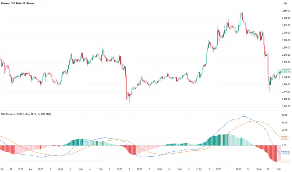
MACD Enhanced [DCAUT]█ MACD Enhanced
📊 ORIGINALITY & INNOVATION
The MACD Enhanced represents a significant improvement over traditional MACD implementations. While Gerald Appel's original MACD from the 1970s was limited to exponential moving averages (EMA), this enhanced version expands algorithmic options by supporting 21 different moving average calculations for both the main MACD line and signal line independently.
This improvement addresses an important limitation of traditional MACD: the inability to adapt the indicator's mathematical foundation to different market conditions. By allowing traders to select from algorithms ranging from simple moving averages (SMA) for stability to advanced adaptive filters like Kalman Filter for noise reduction, this implementation changes MACD from a fixed-algorithm tool into a flexible instrument that can be adjusted for specific market environments and trading strategies.
The enhanced histogram visualization system uses a four-color gradient that helps communicate momentum strength and direction more clearly than traditional single-color histograms.
📐 MATHEMATICAL FOUNDATION
The core calculation maintains the proven MACD formula: Fast MA(source, fastLength) - Slow MA(source, slowLength), but extends it with algorithmic flexibility. The signal line applies the selected smoothing algorithm to the MACD line over the specified signal period, while the histogram represents the difference between MACD and signal lines.
Available Algorithms:
The implementation supports a comprehensive spectrum of technical analysis algorithms:
Basic Averages: SMA (arithmetic mean), EMA (exponential weighting), RMA (Wilder's smoothing), WMA (linear weighting)
Advanced Averages: HMA (Hull's low-lag), VWMA (volume-weighted), ALMA (Arnaud Legoux adaptive)
Mathematical Filters: LSMA (least squares regression), DEMA (double exponential), TEMA (triple exponential), ZLEMA (zero-lag exponential)
Adaptive Systems: T3 (Tillson T3), FRAMA (fractal adaptive), KAMA (Kaufman adaptive), MCGINLEY_DYNAMIC (reactive to volatility)
Signal Processing: ULTIMATE_SMOOTHER (low-pass filter), LAGUERRE_FILTER (four-pole IIR), SUPER_SMOOTHER (two-pole Butterworth), KALMAN_FILTER (state-space estimation)
Specialized: TMA (triangular moving average), LAGUERRE_BINOMIAL_FILTER (binomial smoothing)
Each algorithm responds differently to price action, allowing traders to match the indicator's behavior to market characteristics: trending markets benefit from responsive algorithms like EMA or HMA, while ranging markets require stable algorithms like SMA or RMA.
📊 COMPREHENSIVE SIGNAL ANALYSIS
Histogram Interpretation:
Positive Values: Indicate bullish momentum when MACD line exceeds signal line, suggesting upward price pressure and potential buying opportunities
Negative Values: Reflect bearish momentum when MACD line falls below signal line, indicating downward pressure and potential selling opportunities
Zero Line Crosses: MACD crossing above zero suggests transition to bullish bias, while crossing below indicates bearish bias shift
Momentum Changes: Rising histogram (regardless of positive/negative) signals accelerating momentum in the current direction, while declining histogram warns of momentum deceleration
Advanced Signal Recognition:
Divergences: Price making new highs/lows while MACD fails to confirm often precedes trend reversals
Convergence Patterns: MACD line approaching signal line suggests impending crossover and potential trade setup
Histogram Peaks: Extreme histogram values often mark momentum exhaustion points and potential reversal zones
🎯 STRATEGIC APPLICATIONS
Comprehensive Trend Confirmation Strategies:
Primary Trend Validation Protocol:
Identify primary trend direction using higher timeframe (4H or Daily) MACD position relative to zero line
Confirm trend strength by analyzing histogram progression: consistent expansion indicates strong momentum, contraction suggests weakening
Use secondary confirmation from MACD line angle: steep angles (>45°) indicate strong trends, shallow angles suggest consolidation
Validate with price structure: trending markets show consistent higher highs/higher lows (uptrend) or lower highs/lower lows (downtrend)
Entry Timing Techniques:
Pullback Entries in Uptrends: Wait for MACD histogram to decline toward zero line without crossing, then enter on histogram expansion with MACD line still above zero
Breakout Confirmations: Use MACD line crossing above zero as confirmation of upward breakouts from consolidation patterns
Continuation Signals: Look for MACD line re-acceleration (steepening angle) after brief consolidation periods as trend continuation signals
Advanced Divergence Trading Systems:
Regular Divergence Recognition:
Bullish Regular Divergence: Price creates lower lows while MACD line forms higher lows. This pattern is traditionally considered a potential upward reversal signal, but should be combined with other confirmation signals
Bearish Regular Divergence: Price makes higher highs while MACD shows lower highs. This pattern is traditionally considered a potential downward reversal signal, but trading decisions should incorporate proper risk management
Hidden Divergence Strategies:
Bullish Hidden Divergence: Price shows higher lows while MACD displays lower lows, indicating trend continuation potential. Use for adding to existing long positions during pullbacks
Bearish Hidden Divergence: Price creates lower highs while MACD forms higher highs, suggesting downtrend continuation. Optimal for adding to short positions during bear market rallies
Multi-Timeframe Coordination Framework:
Three-Timeframe Analysis Structure:
Primary Timeframe (Daily): Determine overall market bias and major trend direction. Only trade in alignment with daily MACD direction
Secondary Timeframe (4H): Identify intermediate trend changes and major entry opportunities. Use for position sizing decisions
Execution Timeframe (1H): Precise entry and exit timing. Look for MACD line crossovers that align with higher timeframe bias
Timeframe Synchronization Rules:
Daily MACD above zero + 4H MACD rising = Strong uptrend context for long positions
Daily MACD below zero + 4H MACD declining = Strong downtrend context for short positions
Conflicting signals between timeframes = Wait for alignment or use smaller position sizes
1H MACD signals only valid when aligned with both higher timeframes
Algorithm Considerations by Market Type:
Trending Markets: Responsive algorithms like EMA, HMA may be considered, but effectiveness should be tested for specific market conditions
Volatile Markets: Noise-reducing algorithms like KALMAN_FILTER, SUPER_SMOOTHER may help reduce false signals, though results vary by market
Range-Bound Markets: Stability-focused algorithms like SMA, RMA may provide smoother signals, but individual testing is required
Short Timeframes: Low-lag algorithms like ZLEMA, T3 theoretically respond faster but may also increase noise
Important Note: All algorithm choices and parameter settings should be thoroughly backtested and validated based on specific trading strategies, market conditions, and individual risk tolerance. Different market environments and trading styles may require different configuration approaches.
📋 DETAILED PARAMETER CONFIGURATION
Comprehensive Source Selection Strategy:
Price Source Analysis and Optimization:
Close Price (Default): Most commonly used, reflects final market sentiment of each period. Best for end-of-day analysis, swing trading, daily/weekly timeframes. Advantages: widely accepted standard, good for backtesting comparisons. Disadvantages: ignores intraday price action, may miss important highs/lows
HL2 (High+Low)/2: Midpoint of the trading range, reduces impact of opening gaps and closing spikes. Best for volatile markets, gap-prone assets, forex markets. Calculation impact: smoother MACD signals, reduced noise from price spikes. Optimal when asset shows frequent gaps, high volatility during specific sessions
HLC3 (High+Low+Close)/3: Weighted average emphasizing the close while including range information. Best for balanced analysis, most asset classes, medium-term trading. Mathematical effect: 33% weight to high/low, 33% to close, provides compromise between close and HL2. Use when standard close is too noisy but HL2 is too smooth
OHLC4 (Open+High+Low+Close)/4: True average of all price points, most comprehensive view. Best for complete price representation, algorithmic trading, statistical analysis. Considerations: includes opening sentiment, smoothest of all options but potentially less responsive. Optimal for markets with significant opening moves, comprehensive trend analysis
Parameter Configuration Principles:
Important Note: Different moving average algorithms have distinct mathematical characteristics and response patterns. The same parameter settings may produce vastly different results when using different algorithms. When switching algorithms, parameter settings should be re-evaluated and tested for appropriateness.
Length Parameter Considerations:
Fast Length (Default 12): Shorter periods provide faster response but may increase noise and false signals, longer periods offer more stable signals but slower response, different algorithms respond differently to the same parameters and may require adjustment
Slow Length (Default 26): Should maintain a reasonable proportional relationship with fast length, different timeframes may require different parameter configurations, algorithm characteristics influence optimal length settings
Signal Length (Default 9): Shorter lengths produce more frequent crossovers but may increase false signals, longer lengths provide better signal confirmation but slower response, should be adjusted based on trading style and chosen algorithm characteristics
Comprehensive Algorithm Selection Framework:
MACD Line Algorithm Decision Matrix:
EMA (Standard Choice): Mathematical properties: exponential weighting, recent price emphasis. Best for general use, traditional MACD behavior, backtesting compatibility. Performance characteristics: good balance of speed and smoothness, widely understood behavior
SMA (Stability Focus): Equal weighting of all periods, maximum smoothness. Best for ranging markets, noise reduction, conservative trading. Trade-offs: slower signal generation, reduced sensitivity to recent price changes
HMA (Speed Optimized): Hull Moving Average, designed for reduced lag. Best for trending markets, quick reversals, active trading. Technical advantage: square root period weighting, faster trend detection. Caution: can be more sensitive to noise
KAMA (Adaptive): Kaufman Adaptive MA, adjusts smoothing based on market efficiency. Best for varying market conditions, algorithmic trading. Mechanism: fast smoothing in trends, slow smoothing in sideways markets. Complexity: requires understanding of efficiency ratio
Signal Line Algorithm Optimization Strategies:
Matching Strategy: Use same algorithm for both MACD and signal lines. Benefits: consistent mathematical properties, predictable behavior. Best when backtesting historical strategies, maintaining traditional MACD characteristics
Contrast Strategy: Use different algorithms for optimization. Common combinations: MACD=EMA, Signal=SMA for smoother crossovers, MACD=HMA, Signal=RMA for balanced speed/stability, Advanced: MACD=KAMA, Signal=T3 for adaptive behavior with smooth signals
Market Regime Adaptation: Trending markets: both fast algorithms (EMA/HMA), Volatile markets: MACD=KALMAN_FILTER, Signal=SUPER_SMOOTHER, Range-bound: both slow algorithms (SMA/RMA)
Parameter Sensitivity Considerations:
Impact of Parameter Changes:
Length Parameter Sensitivity: Small parameter adjustments can significantly affect signal timing, while larger adjustments may fundamentally change indicator behavior characteristics
Algorithm Sensitivity: Different algorithms produce different signal characteristics. Thoroughly test the impact on your trading strategy before switching algorithms
Combined Effects: Changing multiple parameters simultaneously can create unexpected effects. Recommendation: adjust parameters one at a time and thoroughly test each change
📈 PERFORMANCE ANALYSIS & COMPETITIVE ADVANTAGES
Response Characteristics by Algorithm:
Fastest Response: ZLEMA, HMA, T3 - minimal lag but higher noise
Balanced Performance: EMA, DEMA, TEMA - good trade-off between speed and stability
Highest Stability: SMA, RMA, TMA - reduced noise but increased lag
Adaptive Behavior: KAMA, FRAMA, MCGINLEY_DYNAMIC - automatically adjust to market conditions
Noise Filtering Capabilities:
Advanced algorithms like KALMAN_FILTER and SUPER_SMOOTHER help reduce false signals compared to traditional EMA-based MACD. Noise-reducing algorithms can provide more stable signals in volatile market conditions, though results will vary based on market conditions and parameter settings.
Market Condition Adaptability:
Unlike fixed-algorithm MACD, this enhanced version allows real-time optimization. Trending markets benefit from responsive algorithms (EMA, HMA), while ranging markets perform better with stable algorithms (SMA, RMA). The ability to switch algorithms without changing indicators provides greater flexibility.
Comparative Performance vs Traditional MACD:
Algorithm Flexibility: 21 algorithms vs 1 fixed EMA
Signal Quality: Reduced false signals through noise filtering algorithms
Market Adaptability: Optimizable for any market condition vs fixed behavior
Customization Options: Independent algorithm selection for MACD and signal lines vs forced matching
Professional Features: Advanced color coding, multiple alert conditions, comprehensive parameter control
USAGE NOTES
This indicator is designed for technical analysis and educational purposes. Like all technical indicators, it has limitations and should not be used as the sole basis for trading decisions. Algorithm performance varies with market conditions, and past characteristics do not guarantee future results. Always combine with proper risk management and thorough strategy testing.
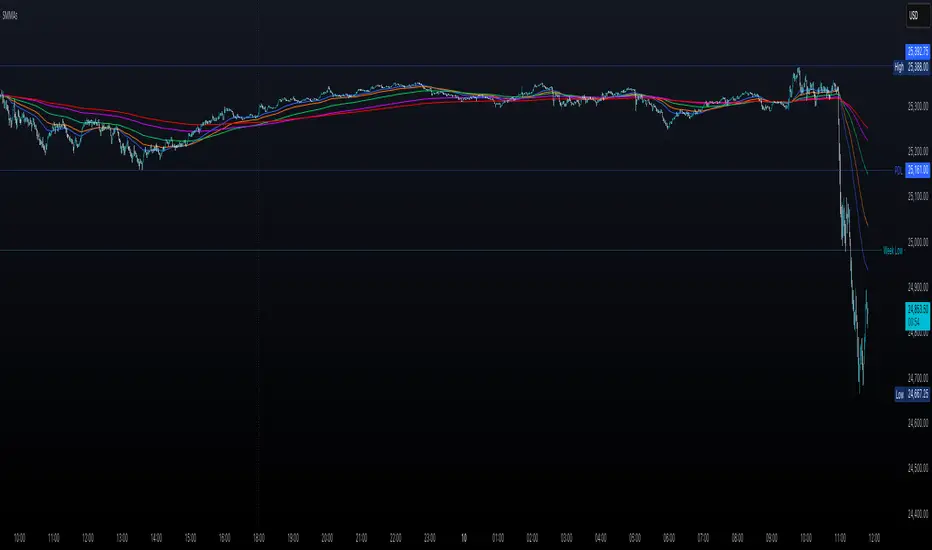
Multiple Smoothed Moving AveragesMultiple Smoothed Moving Averages (SMMAs)
This indicator displays up to 5 Smoothed Moving Averages (SMMAs) on your chart, providing a comprehensive view of multiple trend timeframes simultaneously.
═══════════════════════════════════════
WHAT IS A SMOOTHED MOVING AVERAGE?
═══════════════════════════════════════
The Smoothed Moving Average (SMMA), also known as the Running Moving Average (RMA), is a type of moving average that provides more smoothing than a Simple Moving Average (SMA).
Unlike SMA which gives equal weight to all values in the period, SMMA uses a recursive formula that gives more weight to previous SMMA values, resulting in:
- Smoother price action with less noise
- Slower response to recent price changes
- Better identification of longer-term trends
- Reduced false signals in choppy markets
CALCULATION METHOD:
- First value: Simple Moving Average of the initial period
- Subsequent values: (Previous SMMA × (Length - 1) + Current Price) / Length
This recursive nature makes SMMA particularly effective for identifying sustained trends while filtering out short-term volatility.
═══════════════════════════════════════
FEATURES
═══════════════════════════════════════
✓ 5 Independent SMMAs: Each with its own configurable period length
✓ Individual Toggles: Show/hide each SMMA independently
✓ Distinct Colors: Easy visual identification of each moving average
✓ Customizable Lengths: Adjust each period to match your trading strategy
✓ Shared Source: All SMMAs calculate from the same price source (default: close)
✓ Overlay Display: Plots directly on the price chart
═══════════════════════════════════════
DEFAULT SETTINGS
═══════════════════════════════════════
- SMMA 1: 30 periods (Blue)
- SMMA 2: 50 periods (Orange)
- SMMA 3: 100 periods (Green)
- SMMA 4: 200 periods (Purple)
- SMMA 5: 300 periods (Red)
All SMMAs are enabled by default.
═══════════════════════════════════════
HOW TO USE
═══════════════════════════════════════
TREND IDENTIFICATION:
- Price above all SMMAs = Strong uptrend
- Price below all SMMAs = Strong downtrend
- Price between SMMAs = Transitional phase or consolidation
SUPPORT & RESISTANCE:
- SMMAs often act as dynamic support in uptrends
- SMMAs often act as dynamic resistance in downtrends
- Longer-period SMMAs (200, 300) provide stronger S/R levels
CROSSOVER SIGNALS:
- Faster SMMA crossing above slower SMMA = Bullish signal
- Faster SMMA crossing below slower SMMA = Bearish signal
MULTIPLE TIMEFRAME ANALYSIS:
- Short-term trends: 30, 50 periods
- Medium-term trends: 100 periods
- Long-term trends: 200, 300 periods
═══════════════════════════════════════
CUSTOMIZATION
═══════════════════════════════════════
INPUTS TAB:
- Adjust each SMMA length to suit your trading timeframe
- Toggle individual SMMAs on/off using checkboxes
- Change the source (close, open, high, low, hl2, hlc3, ohlc4)
STYLE TAB:
- Modify line colors for each SMMA
- Adjust line thickness and style
- Change transparency levels
═══════════════════════════════════════
NOTES
═══════════════════════════════════════
- This indicator uses the mathematically correct SMMA calculation with the recursive formula
- All calculations are performed on every bar to ensure data consistency
- SMMAs respond more slowly than EMAs but faster than WMAs to price changes
- Best used in combination with other technical analysis tools
- Use on any timeframe
═══════════════════════════════════════
Perfect for traders who want a clear, multi-timeframe view of market trends using the smooth, reliable SMMA calculation method.
EMA Candle ColorEMA Candle Color - Visual EMA-Based Candle Coloring System
Overview:
This indicator provides a visual approach to trend identification by coloring candles based on their relationship with an Exponential Moving Average (EMA). The script dynamically colors both the candle bars and plots custom candles to give traders an immediate visual representation of price momentum relative to the EMA.
How It Works:
The indicator calculates an EMA based on your chosen source (default: open price) and length (default: 10 periods). It then applies a simple yet effective rule:
When the source price is ABOVE the EMA → Candles turn GREEN (bullish)
When the source price is BELOW the EMA → Candles turn RED (bearish)
This instant visual feedback helps traders quickly identify:
Current trend direction
Potential support/resistance levels (the EMA line itself)
Momentum shifts when candles change color
Key Features:
Customizable EMA Parameters: Adjust the EMA length (1-500) and source (open, close, high, low, hl2, hlc3, ohlc4)
Custom Color Selection: Choose your preferred bullish and bearish colors to match your chart theme
Dual Visualization: Both bar coloring and custom plotcandle for enhanced visibility
Offset Capability: Shift the EMA line forward or backward for advanced analysis
Clean Design: Minimal overlay that doesn't clutter your chart
How to Use:
1. Add the indicator to your chart
2. Adjust the EMA Length based on your trading timeframe:
- Shorter periods (5-20) for day trading and scalping
- Medium periods (20-50) for swing trading
- Longer periods (50-200) for position trading
3. Watch for candle color changes as potential entry/exit signals
4. Combine with other indicators for confirmation
Trading Applications:
Trend Following: Stay in trades while candles remain the same color
Reversal Signals: Watch for color changes as early reversal warnings
Filter System: Only take long positions during green candles, shorts during red
Visual Clarity: Quickly assess market sentiment at a glance
Settings:
Length: EMA calculation period (default: 10)
Source: Price data used for EMA calculation (default: open)
Offset: Shift EMA line on chart (default: 0)
Bullish Color: Color for candles above EMA (default: green)
Bearish Color: Color for candles below EMA (default: red)
Technical Details:
The script uses Pine Script v6 and employs the standard ta.ema() function for smooth, responsive EMA calculations. The candle coloring is achieved through both barcolor() and plotcandle() functions, ensuring visibility across different chart settings.
Note:
This indicator works on all timeframes and instruments. For best results, combine with proper risk management and additional confirmation indicators. The EMA Candle Color system is designed to simplify trend identification, not as a standalone trading system.
Tips:
Use on higher timeframes for more reliable signals
Combine with volume analysis for confirmation
Consider using multiple EMA periods for confluence
Disable default candles if using the plotcandle feature to avoid overlap
This script is open-source. Feel free to use it as a foundation for your own trading system or modify it to suit your specific trading style.
Oscillator CandlesticksI've always wondered why we don't use candlesticks for oscillators...then I stopped wondering and made an oscillator with candlesticks.
The following oscillators are available as a proof of concept:
* Consumer Channel Index (CCI)
* Rate of Change (ROC)
* Relative Strength Index (RSI)
* Trend Strength Index (TSI)
You can add a moving average to the ohlc4 value of the oscillator and choose the type of the moving average and whether it should be influenced by volume.

Kalman Filter [DCAUT]█ Kalman Filter
📊 ORIGINALITY & INNOVATION
The Kalman Filter represents an important adaptation of aerospace signal processing technology to financial market analysis. Originally developed by Rudolf E. Kalman in 1960 for navigation and guidance systems, this implementation brings the algorithm's noise reduction capabilities to price trend analysis.
This implementation addresses a common challenge in technical analysis: the trade-off between smoothness and responsiveness. Traditional moving averages must choose between being smooth (with increased lag) or responsive (with increased noise). The Kalman Filter improves upon this limitation through its recursive estimation approach, which continuously balances historical trend information with current price data based on configurable noise parameters.
The key advancement lies in the algorithm's adaptive weighting mechanism. Rather than applying fixed weights to historical data like conventional moving averages, the Kalman Filter dynamically adjusts its trust between the predicted trend and observed prices. This allows it to provide smoother signals during stable periods while maintaining responsiveness during genuine trend changes, helping to reduce whipsaws in ranging markets while not missing significant price movements.
📐 MATHEMATICAL FOUNDATION
The Kalman Filter operates through a two-phase recursive process:
Prediction Phase:
The algorithm first predicts the next state based on the previous estimate:
State Prediction: Estimates the next value based on current trend
Error Covariance Prediction: Calculates uncertainty in the prediction
Update Phase:
Then updates the prediction based on new price observations:
Kalman Gain Calculation: Determines the weight given to new measurements
State Update: Combines prediction with observation based on calculated gain
Error Covariance Update: Adjusts uncertainty estimate for next iteration
Core Parameters:
Process Noise (Q): Represents uncertainty in the trend model itself. Higher values indicate the trend can change more rapidly, making the filter more responsive to price changes.
Measurement Noise (R): Represents uncertainty in price observations. Higher values indicate less trust in individual price points, resulting in smoother output.
Kalman Gain Formula:
The Kalman Gain determines how much weight to give new observations versus predictions:
K = P(k|k-1) / (P(k|k-1) + R)
Where:
K is the Kalman Gain (0 to 1)
P(k|k-1) is the predicted error covariance
R is the measurement noise parameter
When K approaches 1, the filter trusts new measurements more (responsive).
When K approaches 0, the filter trusts its prediction more (smooth).
This dynamic adjustment mechanism allows the filter to adapt to changing market conditions automatically, providing an advantage over fixed-weight moving averages.
📊 COMPREHENSIVE SIGNAL ANALYSIS
Visual Trend Indication:
The Kalman Filter line provides color-coded trend information:
Green Line: Indicates the filter value is rising, suggesting upward price momentum
Red Line: Indicates the filter value is falling, suggesting downward price momentum
Gray Line: Indicates sideways movement with no clear directional bias
Crossover Signals:
Price-filter crossovers generate trading signals:
Golden Cross: Price crosses above the Kalman Filter line, suggests potential bullish momentum development, may indicate a favorable environment for long positions, filter will naturally turn green as it adapts to price moving higher
Death Cross: Price crosses below the Kalman Filter line, suggests potential bearish momentum development, may indicate consideration for position reduction or shorts, filter will naturally turn red as it adapts to price moving lower
Trend Confirmation:
The filter serves as a dynamic trend baseline:
Price Consistently Above Filter: Confirms established uptrend
Price Consistently Below Filter: Confirms established downtrend
Frequent Crossovers: Suggests ranging or choppy market conditions
Signal Reliability Factors:
Signal quality varies based on market conditions:
Higher reliability in trending markets with sustained directional moves
Lower reliability in choppy, range-bound conditions with frequent reversals
Parameter adjustment can help adapt to different market volatility levels
🎯 STRATEGIC APPLICATIONS
Trend Following Strategy:
Use the Kalman Filter as a dynamic trend baseline:
Enter long positions when price crosses above the filter
Enter short positions when price crosses below the filter
Exit when price crosses back through the filter in the opposite direction
Monitor filter slope (color) for trend strength confirmation
Dynamic Support/Resistance:
The filter can act as a moving support or resistance level:
In uptrends: Filter often provides dynamic support for pullbacks
In downtrends: Filter often provides dynamic resistance for bounces
Price rejections from the filter can offer entry opportunities in trend direction
Filter breaches may signal potential trend reversals
Multi-Timeframe Analysis:
Combine Kalman Filters across different timeframes:
Higher timeframe filter identifies primary trend direction
Lower timeframe filter provides precise entry and exit timing
Trade only in direction of higher timeframe trend for better probability
Use lower timeframe crossovers for position entry/exit within major trend
Volatility-Adjusted Configuration:
Adapt parameters to match market conditions:
Low Volatility Markets (Forex majors, stable stocks): Use lower process noise for stability, use lower measurement noise for sensitivity
Medium Volatility Markets (Most equities): Process noise default (0.05) provides balanced performance, measurement noise default (1.0) for general-purpose filtering
High Volatility Markets (Cryptocurrencies, volatile stocks): Use higher process noise for responsiveness, use higher measurement noise for noise reduction
Risk Management Integration:
Use filter as a trailing stop-loss level in trending markets
Tighten stops when price moves significantly away from filter (overextension)
Wider stops in early trend formation when filter is just establishing direction
Consider position sizing based on distance between price and filter
📋 DETAILED PARAMETER CONFIGURATION
Source Selection:
Determines which price data feeds the algorithm:
OHLC4 (default): Uses average of open, high, low, close for balanced representation
Close: Focuses purely on closing prices for end-of-period analysis
HL2: Uses midpoint of high and low for range-based analysis
HLC3: Typical price, gives more weight to closing price
HLCC4: Weighted close price, emphasizes closing values
Process Noise (Q) - Adaptation Speed Control:
This parameter controls how quickly the filter adapts to changes:
Technical Meaning:
Represents uncertainty in the underlying trend model
Higher values allow the estimated trend to change more rapidly
Lower values assume the trend is more stable and slow-changing
Practical Impact:
Lower Values: Produces very smooth output with minimal noise, slower to respond to genuine trend changes, best for long-term trend identification, reduces false signals in choppy markets
Medium Values: Balanced responsiveness and smoothness, suitable for swing trading applications, default (0.05) works well for most markets
Higher Values: More responsive to price changes, may produce more false signals in ranging markets, better for short-term trading and day trading, captures trend changes earlier, adjust freely based on market characteristics
Measurement Noise (R) - Smoothing Control:
This parameter controls how much the filter trusts individual price observations:
Technical Meaning:
Represents uncertainty in price measurements
Higher values indicate less trust in individual price points
Lower values make each price observation more influential
Practical Impact:
Lower Values: More reactive to each price change, less smoothing with more noise in output, may produce choppy signals
Medium Values: Balanced smoothing and responsiveness, default (1.0) provides general-purpose filtering
Higher Values: Heavy smoothing for very noisy markets, reduces whipsaws significantly but increases lag in trend change detection, best for cryptocurrency and highly volatile assets, can use larger values for extreme smoothing
Parameter Interaction:
The ratio between Process Noise and Measurement Noise determines overall behavior:
High Q / Low R: Very responsive, minimal smoothing
Low Q / High R: Very smooth, maximum lag reduction
Balanced Q and R: Middle ground for most applications
Optimization Guidelines:
Start with default values (Q=0.05, R=1.0)
If too many false signals: Increase R or decrease Q
If missing trend changes: Decrease R or increase Q
Test across different market conditions before live use
Consider different settings for different timeframes
📈 PERFORMANCE ANALYSIS & COMPETITIVE ADVANTAGES
Comparison with Traditional Moving Averages:
Versus Simple Moving Average (SMA):
The Kalman Filter typically responds faster to genuine trend changes
Produces smoother output than SMA of comparable length
Better noise reduction in ranging markets
More configurable for different market conditions
Versus Exponential Moving Average (EMA):
Similar responsiveness but with better noise filtering
Less prone to whipsaws in choppy conditions
More adaptable through dual parameter control (Q and R)
Can be tuned to match or exceed EMA responsiveness while maintaining smoothness
Versus Hull Moving Average (HMA):
Different noise reduction approach (recursive estimation vs. weighted calculation)
Kalman Filter offers more intuitive parameter adjustment
Both reduce lag effectively, but through different mechanisms
Kalman Filter may handle sudden volatility changes more gracefully
Response Characteristics:
Lag Time: Moderate and configurable through parameter adjustment
Noise Reduction: Good to excellent, particularly in volatile conditions
Trend Detection: Effective across multiple timeframes
False Signal Rate: Typically lower than simple moving averages in ranging markets
Computational Efficiency: Efficient recursive calculation suitable for real-time use
Optimal Use Cases:
Markets with mixed trending and ranging periods
Assets with moderate to high volatility requiring noise filtering
Multi-timeframe analysis requiring consistent methodology
Systematic trading strategies needing reliable trend identification
Situations requiring balance between responsiveness and smoothness
Known Limitations:
Parameters require adjustment for different market volatility levels
May still produce false signals during extreme choppy conditions
No single parameter set works optimally for all market conditions
Requires complementary indicators for comprehensive analysis
Historical performance characteristics may not persist in changing market conditions
USAGE NOTES
This indicator is designed for technical analysis and educational purposes. The Kalman Filter's effectiveness varies with market conditions, tending to perform better in markets with clear trending phases interrupted by consolidation. Like all technical indicators, it has limitations and should not be used as the sole basis for trading decisions, but rather as part of a comprehensive trading approach.
Algorithm performance varies with market conditions, and past characteristics do not guarantee future results. Always test thoroughly with different parameter settings across various market conditions before using in live trading. No technical indicator can predict future price movements with certainty, and all trading involves risk of loss.
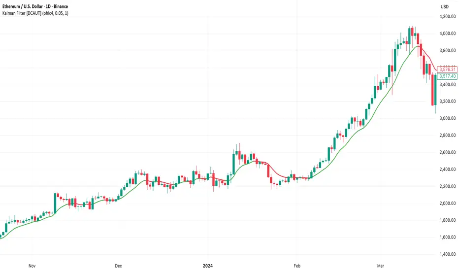
MAMA [DCAUT]█ MAMA (MESA Adaptive Moving Average)
📊 OVERVIEW
The MESA Adaptive Moving Average (MAMA) represents an advanced implementation of John F. Ehlers' adaptive moving average system using the Hilbert Transform Discriminator. This indicator automatically adjusts to market cycles, providing superior responsiveness compared to traditional fixed-period moving averages while maintaining smoothness.
MAMA dynamically calculates two lines: the fast-adapting MAMA line and the following FAMA (Following Adaptive Moving Average) line. The system's core strength lies in its ability to automatically detect and adapt to the dominant market cycle, reducing lag during trending periods while providing stability during consolidation phases.
🎯 CORE CONCEPTS
Signal Interpretation:
• MAMA above FAMA: Indicates bullish trend momentum with the fast line leading upward movement
• MAMA below FAMA: Suggests bearish trend momentum with the fast line leading downward movement
• Golden Cross: MAMA crossing above FAMA signals potential upward momentum shift
• Death Cross: MAMA crossing below FAMA indicates potential downward momentum shift
• Line Convergence: MAMA and FAMA approaching each other suggests trend consolidation or potential reversal
Primary Applications:
• Trend Following: Enhanced responsiveness to trend changes compared to traditional moving averages
• Crossover Signals: MAMA/FAMA crossovers for identifying potential entry and exit points
• Cycle Analysis: Automatic adaptation to market's dominant cycle characteristics
• Reduced Lag: Minimized delay in trend detection while maintaining signal smoothness
📐 MATHEMATICAL FOUNDATION
Hilbert Transform Discriminator Technology:
The MAMA system employs John F. Ehlers' Hilbert Transform Discriminator, a sophisticated signal processing technique borrowed from telecommunications engineering. The Hilbert Transform creates a complex representation of the price series by generating a 90-degree phase-shifted version of the original signal, enabling precise cycle measurement.
The discriminator analyzes the instantaneous phase relationships between the original price series and its Hilbert Transform counterpart. This mathematical relationship reveals the dominant cycle period present in the market data at each point in time, forming the foundation for adaptive smoothing.
Instantaneous Period Calculation:
The algorithm computes the instantaneous period using the arctangent of the ratio between the Hilbert Transform and the original price series. This calculation produces a real-time measurement of the market's dominant cycle, typically ranging from short-term noise cycles to longer-term trend cycles.
The instantaneous period measurement undergoes additional smoothing to prevent erratic behavior from single-bar anomalies. This smoothed period value becomes the basis for calculating the adaptive alpha coefficient that controls the moving average's responsiveness.
Dynamic Alpha Coefficient System:
The adaptive alpha calculation represents the core mathematical innovation of MAMA. The alpha coefficient is derived from the instantaneous period measurement and constrained within the user-defined fast and slow limits.
The mathematical relationship converts the measured cycle period into an appropriate smoothing factor: shorter detected cycles result in higher alpha values (increased responsiveness), while longer cycles produce lower alpha values (increased stability). This creates an automatic adaptation mechanism that responds to changing market conditions.
MAMA/FAMA Calculation Process:
The MAMA line applies the dynamically calculated alpha coefficient to an exponential moving average formula: MAMA = alpha × Price + (1 - alpha) × MAMA . The FAMA line then applies a secondary smoothing operation to the MAMA line, creating a following average that provides confirmation signals.
This dual-line approach ensures that the fast-adapting MAMA line captures trend changes quickly, while the FAMA line offers a smoother confirmation signal, reducing the likelihood of acting on temporary price fluctuations.
Cycle Detection Mechanism:
The underlying cycle detection employs quadrature components derived from the Hilbert Transform to measure both amplitude and phase characteristics of price movements. This allows the system to distinguish between genuine trend changes and temporary price noise, automatically adjusting the smoothing intensity accordingly.
The mathematical framework ensures that during strong trending periods with clear directional movement, the algorithm reduces smoothing to minimize lag. Conversely, during consolidation phases with mixed signals, increased smoothing helps filter out false breakouts and whipsaws.
📋 PARAMETER CONFIGURATION
Source Selection Strategy:
• HL2 (High+Low)/2 (Default): Recommended for cycle analysis as it represents the midpoint of each period's trading range, reducing impact of opening gaps and closing spikes
• Close Price: Traditional choice reflecting final market sentiment, suitable for end-of-day analysis
• HLC3 (High+Low+Close)/3: Balanced approach incorporating range information with closing emphasis
• OHLC4 (Open+High+Low+Close)/4: Most comprehensive price representation for complete market view
Fast Limit Configuration (Default 0.5):
Controls the maximum responsiveness of the adaptive system. Higher values increase sensitivity to recent price changes but may introduce more noise. This parameter sets the upper bound for the dynamic alpha calculation.
Slow Limit Configuration (Default 0.05):
Determines the minimum responsiveness, providing stability during uncertain market conditions. Lower values increase smoothing but may cause delayed signals. This parameter sets the lower bound for the dynamic alpha calculation.
Parameter Relationship Considerations:
The fast and slow limits work together to define the adaptive range. The wider the range between these limits, the more dramatic the adaptation between trending and consolidating market conditions. Different market characteristics may benefit from different parameter configurations, requiring individual testing and validation.
📊 COLOR CODING SYSTEM
Line Visualization:
• Green Line (MAMA): The fast-adapting moving average that responds quickly to price changes
• Red Line (FAMA): The following adaptive moving average that provides confirmation signals
The fixed color scheme provides consistent visual identification of each line, enabling clear differentiation between the fast-adapting MAMA and the following FAMA throughout all market conditions.
💡 CORE VALUE PROPOSITION
Advantages Over Traditional Moving Averages:
• Cycle Adaptation: Automatically adjusts to market's dominant cycle rather than using fixed periods
• Reduced Lag: Faster response to genuine trend changes while filtering market noise
• Mathematical Foundation: Based on advanced signal processing techniques from telecommunications engineering
• Dual-Line System: Provides both fast adaptation (MAMA) and confirmation (FAMA) in one indicator
Comparative Performance Characteristics:
Unlike fixed-period moving averages that apply the same smoothing regardless of market conditions, MAMA adapts its behavior based on current market cycle characteristics. This may help reduce whipsaws during consolidation periods while maintaining responsiveness during trending phases.
Usage Considerations:
This indicator is designed for technical analysis purposes. The adaptive nature means that parameter optimization should consider the specific characteristics of the asset and timeframe being analyzed. Like all technical indicators, MAMA should be used as part of a comprehensive analysis approach rather than as a standalone signal generator.
Alert Functionality:
The indicator includes alert conditions for MAMA/FAMA crossovers, enabling automated notification of potential momentum shifts. These alerts can assist in timing analysis but should be combined with other forms of market analysis for decision-making purposes.
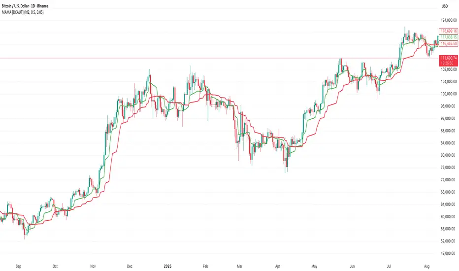
Volume-Weighted RSI & Multi-Normalized MACD### Description for Publishing: Volume-Weighted RSI & Multi-Normalized MACD
**Overview**
The "Volume-Weighted RSI & Multi-Normalized MACD" indicator is a powerful and versatile tool designed for traders seeking enhanced momentum and trend analysis. Combining a volume-weighted Relative Strength Index (VW-RSI) with a customizable Moving Average Convergence Divergence (MACD) featuring multiple normalization methods, this indicator provides deep insights into market dynamics. It supports multi-timeframe (MTF) analysis and includes an optional stepped plotting mode for discrete signal visualization, making it ideal for both trend-following and mean-reversion strategies across various markets (stocks, forex, crypto, etc.).
**Key Features**
1. **Volume-Weighted RSI (VW-RSI)**:
- A modified RSI that incorporates trading volume for greater sensitivity to market activity.
- Normalized to a user-defined range (default: -50 to +50) for consistent analysis.
- Optional smoothing with multiple moving average types (SMA, EMA, WMA, VWMA, SMMA, or SMA with Bollinger Bands) to reduce noise and highlight trends.
- Overbought (+20) and oversold (-20) levels for quick reference.
2. **Multi-Normalized MACD**:
- Offers six normalization methods for MACD, allowing traders to tailor the output to their strategy:
- Normalized Volume Weighted MACD (unbounded).
- Min-Max Normalization (bounded).
- Volatility Normalization (unbounded, volatility-adjusted).
- Volatility Normalization with Min-Max (bounded).
- Hyperbolic Tangent Normalization (bounded).
- Arctangent Normalization (bounded).
- Min-Max with Smoothing (bounded).
- All bounded methods scale to the user-defined range (default: -50 to +50), ensuring comparability with VW-RSI.
- Dynamic color changes for MACD line (lime/red) and histogram (aqua/blue/red/maroon) based on momentum and signal line crosses.
3. **Stepped Plotting Mode**:
- Optional mode to plot RSI and MACD as discrete, stepped lines, reducing noise by only updating when values change significantly (configurable thresholds).
- Ideal for traders focusing on clear, actionable signal changes.
4. **Multi-Timeframe Support**:
- Configurable timeframe input (default: chart timeframe) for analyzing RSI and MACD on higher or lower timeframes, enhancing cross-timeframe strategies.
5. **Customizable Display**:
- Toggle options to show/hide MACD line, signal line, histogram, and cross dots.
- Bollinger Bands for RSI smoothing (optional) with adjustable standard deviation multiplier.
- Clear visual cues with horizontal lines for overbought/oversold levels, midline, and MACD bounds.
**Usage Instructions**
1. **Add to Chart**: Apply the indicator to any symbol (e.g., BTCUSD, SPY) on any timeframe (1H, 1D, etc.).
2. **Configure Settings**:
- **General**: Adjust `Lower Bound` (-50 default) and `Upper Bound` (+50 default) for the output range. Set `Timeframe` for MTF analysis. Enable `Stepped?` for discrete plotting.
- **RSI**: Choose `Price Source` (default: ohlc4), `RSI Length` (default: 9), and smoothing options (e.g., EMA, Bollinger Bands). Adjust `RSI Diff Threshold` for stepped mode.
- **MACD**: Select `Price Source`, `Fast Length` (9), `Slow Length` (21), `Signal Length` (9), and a normalization method (default: Volatility Min-Max). Adjust `MACD Diff Threshold` for stepped mode.
- **Display Options**: Toggle MACD components and histogram colors for clarity.
3. **Interpretation**:
- **VW-RSI**: Watch for crosses above +20 (overbought) or below -20 (oversold) for potential reversals. Use smoothed RSI or Bollinger Bands for trend confirmation.
- **MACD**: Look for MACD/Signal line crosses (dots indicate crossings) and histogram changes for momentum shifts. Bounded normalizations align with RSI for unified analysis.
- **Stepped Mode**: Focus on significant changes in RSI/MACD for clearer signals.
4. **Companion Overlay**: For visualization on the main price chart, use the companion script "VW-RSI & MACD Price Overlay" (available separately, requires this script to be published). It plots RSI and MACD as price-scaled echo lines, with toggles to show/hide and customizable scaling (high/low or ATR).
**Who Is This For?**
- **Trend Traders**: Use MACD normalizations and MTF to identify momentum shifts across timeframes.
- **Mean-Reversion Traders**: Leverage VW-RSI’s overbought/oversold signals for entry/exit points.
- **Technical Analysts**: Customize normalization and smoothing to match specific market conditions.
- **All Markets**: Works on stocks, forex, cryptocurrencies, and more, with any timeframe.
**Notes**
- Unbounded MACD normalizations (`enable_nvw`, `enable_vol`) may produce values outside -50/+50, suitable for volatility-focused strategies.
- For price chart overlay, publish this script and use its ID in the companion script’s `request.security` call.
- Adjust scaling inputs in the companion script for optimal visualization on volatile or stable assets.
**Author’s Note**
Developed by NEPOLIX, this indicator combines volume-weighted precision with flexible normalization for robust technical analysis. Feedback and suggestions are welcome to enhance future versions!
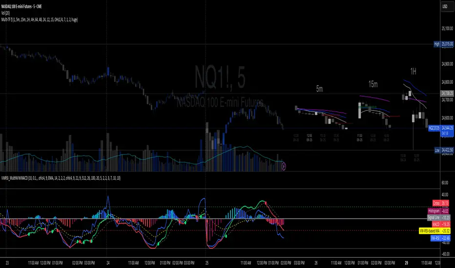
Double Median SD Bands | MisinkoMasterThe Double Median SD Bands (DMSDB) is a trend-following tool designed to capture market direction in a way that balances responsiveness and smoothness, filtering out excessive noise without introducing heavy lag.
Think of it like a house:
A jail (too restrictive) makes you miss opportunities.
No house at all (too unsafe) leaves you exposed to false signals.
DMSDB acts like a comfortable house with windows—protecting you from the noise while still letting you see what’s happening in the market.
🔎 Methodology
The script works in the following steps:
Standard Deviation (SD) Calculation
Computes the standard deviation of the selected price source (ohlc4 by default).
The user can choose whether to use biased (sample) or unbiased (population) standard deviation.
Raw Bands Construction
Upper Band = source + (SD × multiplier)
Lower Band = source - (SD × multiplier)
The multiplier can be adjusted for tighter or looser bands.
First Median Smoothing
Applies a median filter over half of the length (len/2) to both bands.
This reduces noise without creating excessive lag.
Second Median Smoothing
Applies another median filter over √len to the already smoothed bands.
This produces a balance:
Cutting the length → maintains responsiveness.
Median smoothing → reduces whipsaws.
The combination creates a fast yet clean band system ideal for trend detection.
📈 Trend Logic
The trend is detected based on price crossing the smoothed bands:
Long / Bullish (Purple) → when price crosses above the upper band.
Short / Bearish (Gold) → when price crosses below the lower band.
Neutral → when price remains between the bands.
🎨 Visualization
Upper and lower bands are plotted as colored lines.
The area between the bands is filled with a transparent zone that reflects the current bias:
Purple shading = Bullish zone.
Golden shading = Bearish zone.
This creates a visual tunnel for trend confirmation, helping traders quickly identify whether price action is trending or consolidating.
⚡ Features
Adjustable Length parameter (len) for dynamic control.
Adjustable Band Multiplier for volatility adaptation.
Choice between biased vs. unbiased standard deviation.
Double median smoothing for clarity + responsiveness.
Works well on cryptocurrencies (e.g., BTCUSD) but is flexible enough for stocks, forex, and indices.
✅ Use Cases
Trend Following → Ride trends by staying on the correct side of the bands.
Entry Timing → Use crossovers above/below bands for entry triggers.
Filter for Other Strategies → Can serve as a directional filter to avoid trading against the trend.
⚠️ Limitations & Notes
This is a trend-following tool, so it will perform best in trending conditions.
In sideways or choppy markets, whipsaws may still occur (although smoothing reduces them significantly).
The indicator is not a standalone buy/sell system. For best results, combine with volume, momentum, or higher-timeframe confluence.
All of this makes for a really unique & original tool, as it removes noise but keeps good responsitivity, using methods from many different principles which make for a smooth a very useful tool

Stop Loss Advisor📊 Stop Loss Advisor - Advanced Risk Management Tool
A sophisticated Pine Script v5 indicator designed to suggest optimal stop loss distances based on market volatility, combining ATR and Standard Deviation analysis for precise risk management.
🎯 What Makes This Different from Bollinger Bands?
While Bollinger Bands focus on mean reversion and overbought/oversold conditions using a moving average center line, this indicator is specifically designed for risk management . It creates dynamic bands around the current price to suggest where NOT to place your stop loss, preventing you from being stopped out by normal market noise.
⚡ Key Features
Dynamic ATR Calculation - Fully customizable ATR periods with adaptive volatility filtering
Standard Deviation Integration - Optional StdDev component for enhanced statistical accuracy
Multiple Combination Modes - Average, Maximum, ATR Weighted, or StdDev Weighted
Flexible Price Sources - Choose from Close, HL2, HLC3, or OHLC4
Automatic Pip Calculation - Works across all instruments with automatic pip value detection
Smart Alerts System - Get notified when suggested stop loss exceeds your base risk tolerance
Real-time Information Table - Displays current values and risk status
Visual Labels - Shows exact pip distances directly on chart
Band Smoothing - Prevents erratic movements with customizable averaging
📈 How It Works
ATR Analysis : Calculates Average True Range to measure current market volatility
Statistical Enhancement : Optionally combines with Standard Deviation for more robust calculations
Dynamic Bands : Creates upper and lower bands that expand/contract with volatility
Pip Conversion : Automatically converts distances to pips for easy interpretation
Risk Assessment : Compares suggested distances with your base stop loss tolerance
🔧 Customization Options
ATR Settings:
Customizable ATR period (default: 14)
Adjustable multiplier with 0.1 step precision
Optional volatility filtering for enhanced sensitivity
Standard Deviation (Optional):
Independent period and multiplier settings
Multiple price source options
Four combination modes with ATR
Visual Customization:
Fully customizable colors for all elements
Multiple line styles (solid, dashed, dotted)
Optional band filling with transparency control
Show/hide ATR line overlay
Configurable band smoothing
💡 Perfect For
Forex Traders - Especially effective on major pairs and XAUUSD
Risk Managers - Calculate optimal stop distances before entering trades
Scalpers - Avoid being stopped out by normal market fluctuations
Swing Traders - Adapt stop losses to current volatility conditions
📊 Indicator Values
The information table displays:
Current ATR Value (in pips)
Suggested Long Stop Loss (distance in pips)
Suggested Short Stop Loss (distance in pips)
Risk Status - "SAFE" or "HIGH RISK" based on your base tolerance
Standard Deviation Value (when enabled)
Combination Method (when using both ATR and StdDev)
⚠️ Important Notes
This indicator suggests minimum stop loss distances, not entry/exit signals
Always combine with your trading strategy and risk management rules
Do not use as a standalone trading system
Backtesting recommended before live implementation
Default settings work well for most scenarios, but optimization is encouraged
🎨 Default Configuration
ATR Period: 14
ATR Multiplier: 2.0
Price Source: Close
Base Stop Loss: 20 pips
Band Smoothing: 3 periods
Standard Deviation: Optional (20 period, 2.0 multiplier)
🚀 Getting Started
Add the indicator to your chart
Set your base stop loss tolerance in the settings
Choose your preferred price source and ATR parameters
Enable Standard Deviation for enhanced accuracy (optional)
Monitor the information table for real-time risk assessment
Use the suggested distances as minimum stop loss levels
Pro Tip: In low volatility markets, the bands will contract suggesting tighter stops. In high volatility periods, they expand warning you to use wider stops to avoid being stopped out by normal price action.
📝 Version History & Updates
This indicator is actively maintained and updated based on user feedback. Future enhancements may include multi-timeframe analysis, trend-based asymmetric bands, and additional statistical measures.
Transform your risk management approach with data-driven stop loss suggestions that adapt to real market conditions!

Reverse RSI [R] – Predictive RSI Price LevelsReverse RSI – Predictive RSI Price Levels
Description
This indicator is a modified and enhanced version of the original "Reverse RSI" by Franklin Moormann (cheatcountry), published under the MIT License. It estimates the price levels at which the RSI would reach specific thresholds, typically RSI = 30 (oversold) and RSI = 70 (overbought), based on current market conditions.
Key Features
Calculates price levels corresponding to RSI = 30 and RSI = 70
Helps forecast potential support and resistance zones based on RSI targets
Automatically updates with each new candle
Supports custom RSI length and price source (close, hl2, ohlc4, etc.)
Designed for traders who want to anticipate momentum extremes before they occur
Use Cases
Estimate how far the price must move to reach RSI oversold or overbought levels
Plan limit entries or exits based on projected RSI thresholds
Combine with standard RSI or other indicators for confirmation and analysis
Credits
This script is based on the original "Reverse RSI" by Franklin Moormann (cheatcountry) and released under the MIT License.
Modified and maintained by bitcoinrb.
Penguin Volatility State StrategyThe Penguin Volatility State Strategy is a comprehensive technical analysis framework designed to identify the underlying "state" or "regime" of the market. Instead of just providing simple buy or sell signals, its primary goal is to classify the market into one of four distinct states by combining trend, momentum, and volatility analysis.
The core idea is to trade only when these three elements align, focusing on periods of volatility expansion (a "squeeze breakout") that occur in the direction of a confirmed trend and are supported by strong momentum.
Key Components
The strategy is built upon two main engines
The Volatility Engine (Bollinger Bands vs. Keltner Channels)
This engine detects periods of rapidly increasing volatility. It measures the percentage difference (diff) between the upper bands of Bollinger Bands (which are based on standard deviation) and Keltner Channels (based on Average True Range). During a volatility "squeeze," both bands are close. When price breaks out, the Bollinger Band expands much faster than the Keltner Channel, causing the diff value to become positive. A positive diff signals a volatility breakout, which is the moment the strategy becomes active.
The Trend & Momentum Engine (Multi-EMA System)
This engine determines the market's direction and strength. It uses:
A Fast EMA (e.g., 12-period) and a Slow EMA (e.g., 26-period): The crossover of these two moving averages defines the primary, underlying trend (similar to a MACD).
An Ultra-Fast EMA (e.g., 2-period of ohlc4): This is used to measure the immediate, short-term momentum of the price.
The Four Market States
By combining the Trend and Momentum engines, the strategy categorizes the market into four visually distinct states, represented by the chart's background color. This is the most crucial aspect of the system.
💚 Green State: Strong Bullish
The primary trend is UP (Fast EMA > Slow EMA) AND the immediate momentum is STRONG (Price > Fast EMA).
Interpretation: This represents a healthy, robust uptrend where both the underlying trend and short-term price action are aligned. It is considered the safest condition for taking long positions.
❤️ Red State: Strong Bearish
Condition: The primary trend is DOWN (Fast EMA < Slow EMA) AND the immediate momentum is WEAK (Price < Fast EMA).
Interpretation: This represents a strong, confirmed downtrend. It is considered the safest condition for taking short positions.
💛 Yellow State: Weakening Bullish / Pullback
Condition: The primary trend is UP (Fast EMA > Slow EMA) BUT the immediate momentum is WEAK (Price < Fast EMA).
Interpretation: This is a critical warning signal for bulls. While the larger trend is still up, the short-term price action is showing weakness. This could be a minor pullback, a period of consolidation, or the very beginning of a trend reversal. Caution is advised.
💙 Blue State: Weakening Bearish / Relief Rally
Condition: The primary trend is DOWN (Fast EMA < Slow EMA) BUT the immediate momentum is STRONG (Price > Fast EMA).
Interpretation: This signals that a downtrend is losing steam. It often represents a short-covering rally (a "bear market rally") or the first potential sign of a market bottom. Bears should be cautious and consider taking profits.
How the Strategy Functions
The strategy uses these four states as its foundation for making trading decisions. The entry and exit arrows (Long, Short, Close) are generated based on a set of rules that can be customized by the user. For instance, a trader can configure the strategy to
Only take long trades during the Green State.
Require a confirmed volatility breakout (diff > 0) before entering a trade.
Use the "RSI on Diff" indicator to ensure that the breakout is supported by accelerating momentum.
Summary
In essence, the Penguin Volatility State Strategy provides a powerful "dashboard" for viewing the market. It moves beyond simple indicators to offer a contextual understanding of price action. By waiting for the alignment of Trend (the State), Volatility (the Breakout), and Momentum (the Acceleration), it helps traders to identify higher-probability setups and, just as importantly, to know when it is better to stay out of the market.
License / disclaimer
© waranyu.trkm — MIT License. Educational use only; not financial advice.
3 MA's with Crossing SignalsPlots three fully configurable moving averages on one chart and prints/alerts BUY/SELL signals when price crosses your chosen MA(s). Built to match TradingView’s built-ins exactly.
Features
Per-line MA type: SMA, EMA, SMMA (RMA), WMA, VWMA
Per-line settings: length, color, offset
Source control: Close, Open, High, Low, HL2, HLC3, OHLC4
Optional Heikin Ashi calculation for both the MAs and the cross price
Toggle signals vs MA1 / MA2 / MA3 independently
Alert conditions for every cross (ready for “Once per bar close”)
How signals work
UP when the selected price stream crosses above the chosen MA
DOWN when it crosses below
Signals/alerts follow your selected source (and HA toggle) to keep everything consistent.
VWMA MACD Trend Grinder Buy/Sell SignalsDescription:
This indicator combines a VWMA-based MACD with volume and trend filters to reduce false buy and sell signals.
It is designed to give more reliable entry and exit points in trending markets while avoiding low-volume noise.
Features:
1. VWMA MACD:
- MACD is calculated using Volume-Weighted Moving Averages (VWMA) instead of standard EMAs.
- Histogram shows the difference between MACD and its signal line.
2. Volume Filter:
- Signals are only triggered when current volume exceeds a multiple of its moving average.
- Reduces false signals in low-volume periods.
3. Trend Filter:
- Only triggers buy signals when price is above a long-term VWMA (uptrend).
- Only triggers sell signals when price is below the long-term VWMA (downtrend).
- Helps avoid counter-trend trades.
4. Plots:
- MACD (blue), Signal (orange), Histogram (green/red)
- Trend VWMA (purple)
- Buy and Sell arrows in the indicator pane (green/red)
5. Alerts:
- Configurable alerts for buy and sell signals filtered by volume and trend.
Inputs:
- Fast Length: VWMA period for the fast MACD line (default 12)
- Slow Length: VWMA period for the slow MACD line (default 26)
- Signal Length: EMA period for the MACD signal line (default 9)
- Volume MA Length: Length for volume moving average filter (default 20)
- Volume Threshold Multiplier: Multiplier for volume filter (default 1.2)
- Trend VWMA Length: Period for long-term trend VWMA (default 50)
- Price Source: Close, HL2, HLC3, OHLC4
Usage:
- Use as a confirmation tool along with other analysis techniques.
- Buy when the green triangle appears (MACD crossover, above trend VWMA, sufficient volume).
- Sell when the red triangle appears (MACD crossunder, below trend VWMA, sufficient volume).
- Trend VWMA helps visually confirm the market trend.
VWMA MACD AmanitaVWMA MACD (Volume-Weighted MACD)
This indicator modifies the standard MACD by replacing EMAs with VWMAs
(Volume-Weighted Moving Averages).
- Fast VWMA (default 12 bars)
- Slow VWMA (default 26 bars)
- MACD Line = Fast VWMA - Slow VWMA
- Signal Line = EMA of MACD (default 9 bars)
- Histogram = MACD - Signal
Compared to the standard MACD, this version emphasizes price moves that
are backed by higher trading volume, helping to filter out weak signals.
The script also lets you choose the price source (Close, HL2, HLC3, OHLC4).

Multi Volume Weighted Average Price1. Three independent VWAP configurations (VWAP 1, 2, and 3). Each can be set up separately
for periods such as: session, daily, weekly, monthly, etc.
2. Previous VWAP closing prices: Closed VWAPs from previous periods remain visible until the
price touches them. At that point, they are removed.
3. Bands: Based on standard deviation or a percentage of VWAP with an adjustable multiplier.
The bands can be turned on or off.
4. Source: OHLC4 is the default setting for an accurate approximation, but it is customizable
(e.g. HLC3).
5. Global Setting: Select 10,000 or 20,000 historical bars to prevent runtime errors for long
periods.
Usage tips:
1. Use VWAP 1 for daily sessions, VWAP 2 for weekly, and VWAP 3 for Monthly analysis to receive
multi-timeframe support.
2. Customize the labels to clearly distinguish them (e.g. D VWAP, W VWAP, M VWAP).
3. If you encounter errors with historical data (e.g. on the M1 chart), minimize the number of
historical bars displayed to 10,000.

Mean Reversion & Momentum Hybrid | D_QUANT 📌 Mean Reversion & Momentum Hybrid | D_QUANT
📖 Description:
This indicator combines mean reversion logic, volatility filtering, and percentile-based momentum to deliver clear, context-aware buy/sell signals designed for trend-following and contrarian setups.
At its core, it merges:
A Bollinger Band % Positioning Model (BB%)
A 75th/25th Percentile Momentum System
A Volatility-Adjusted Trend Filter using RMA + ATR
All tied together with a dynamic gradient-style oscillator that visualizes signal strength and persistence over time — making it easy to track high-conviction setups.
Signals only trigger when all three core components align, filtering out noise and emphasizing high-probability turning points or trend continuations.
⚙️ Methodology Overview:
Bollinger Bands % (BB%):
Price is measured as a percentage between upper and lower Bollinger Bands (based on OHLC4). Entries are only considered when price exceeds custom BB% thresholds — emphasizing market extremes.
Volatility-Based Trend Filter (RMA + ATR):
A smoothed RMA baseline is paired with ATR to define trend bias. This ensures signals only occur when price deviates meaningfully beyond recent volatility.
Percentile Momentum Model (75th/25th Rank):
Price is compared against its rolling 75th and 25th percentile. If price breaks these statistical boundaries (adjusted by ATR), it triggers a directional momentum condition.
Signal Consensus Engine:
All three layers must agree — BB% condition, trend filter, and percentile momentum — before a buy or sell signal is plotted.
Gradient Oscillator Visualization:
Signals appear as a fading oscillator line with a gradient-filled area beneath it. The color intensity represents how “fresh” or “strong” the signal is, fading over time if not reconfirmed, offering both clarity and signal aging at a glance.
🔧 User Inputs:
🧠 Core Settings:
Source: Select the price input (default: close)
Bollinger Bands Length: Period for BB basis and deviation
Bollinger Bands Multiplier: Width of the bands
Minimum BB Width (% of Price): Prevents signals during low-volatility chop
📊 BB% Thresholds:
BB% Long Threshold (L): Minimum %B to consider a long
BB% Short Threshold (S): Maximum %B to consider a short
🔍 Trend Filter Parameters:
RMA Length: Period for the smoothed trend baseline
ATR Length: Lookback for ATR in trend deviation filter
⚡️ Momentum Parameters:
Momentum Length: Period for percentile momentum calculation
Mult_75 / Mult_25: ATR-adjusted thresholds for breakout above/below percentile levels
🎨 Visualization:
Bar Coloring: Highlights candles during active signals
Background Coloring: Optional background shading for signals
Show Oscillator Plot: Toggle the gradient-style oscillator
🧪 Use Case:
This indicator works well across all assets for trend identification. It is particularly effective when used on higher timeframes (e.g. 12H, 1D,2D) to capture mean reversion bounces or confirm breakouts backed by percentile momentum and volatility expansion.
⚠️ Notes:
This is not financial advice. Use in combination with proper risk management and confluence from other tools.

Time-Decaying Percentile Oscillator [BackQuant]Time-Decaying Percentile Oscillator
1. Big-picture idea
Traditional percentile or stochastic oscillators treat every bar in the look-back window as equally important. That is fine when markets are slow, but if volatility regime changes quickly yesterday’s print should matter more than last month’s. The Time-Decaying Percentile Oscillator attempts to fix that blind spot by assigning an adjustable weight to every past price before it is ranked. The result is a percentile score that “breathes” with market tempo much faster to flag new extremes yet still smooth enough to ignore random noise.
2. What the script actually does
Build a weight curve
• You pick a look-back length (default 28 bars).
• You decide whether weights fall Linearly , Exponentially , by Power-law or Logarithmically .
• A decay factor (lower = faster fade) shapes how quickly the oldest price loses influence.
• The array is normalised so all weights still sum to 1.
Rank prices by weighted mass
• Every close in the window is paired with its weight.
• The pairs are sorted from low to high.
• The cumulative weight is walked until it equals your chosen percentile level (default 50 = median).
• That price becomes the Time-Decayed Percentile .
Find dispersion with robust statistics
• Instead of a fragile standard deviation the script measures weighted Median-Absolute-Deviation about the new percentile.
• You multiply that deviation by the Deviation Multiplier slider (default 1.0) to get a non-parametric volatility band.
Build an adaptive channel
• Upper band = percentile + (multiplier × deviation)
• Lower band = percentile – (multiplier × deviation)
Normalise into a 0-100 oscillator
• The current close is mapped inside that band:
0 = lower band, 50 = centre, 100 = upper band.
• If the channel squeezes, tiny moves still travel the full scale; if volatility explodes, it automatically widens.
Optional smoothing
• A second-stage moving average (EMA, SMA, DEMA, TEMA, etc.) tames the jitter.
• Length 22 EMA by default—change it to tune reaction speed.
Threshold logic
• Upper Threshold 70 and Lower Threshold 30 separate standard overbought/oversold states.
• Extreme bands 85 and 15 paint background heat when aggressive fade or breakout trades might trigger.
Divergence engine
• Looks back twenty bars.
• Flags Bullish divergence when price makes a lower low but oscillator refuses to confirm (value < 40).
• Flags Bearish divergence when price prints a higher high but oscillator stalls (value > 60).
3. Component walk-through
• Source – Any price series. Close by default, switch to typical price or custom OHLC4 for futures spreads.
• Look-back Period – How many bars to rank. Short = faster, long = slower.
• Base Percentile Level – 50 shows relative position around the median; set to 25 / 75 for quartile tracking or 90 / 10 for extreme tails.
• Deviation Multiplier – Higher values widen the dynamic channel, lowering whipsaw but delaying signals.
• Decay Settings
– Type decides the curve shape. Exponential (default 1.16) mimics EMA logic.
– Factor < 1 shrinks influence faster; > 1 spreads influence flatter.
– Toggle Enable Time Decay off to compare with classic equal-weight stochastic.
• Smoothing Block – Choose one of seven MA flavours plus length.
• Thresholds – Overbought / Oversold / Extreme levels. Push them out when working on very mean-reverting assets like FX; pull them in for trend monsters like crypto.
• Display toggles – Show or hide threshold lines, extreme filler zones, bar colouring, divergence labels.
• Colours – Bullish green, bearish red, neutral grey. Every gradient step is automatically blended to generate a heat map across the 0-100 range.
4. How to read the chart
• Oscillator creeping above 70 = market auctioning near the top of its adaptive range.
• Fast poke above 85 with no follow-through = exhaustion fade candidate.
• Slow grind that lives above 70 for many bars = valid bullish trend, not a fade.
• Cross back through 50 shows balance has shifted; treat it like a micro trend change.
• Divergence arrows add extra confidence when you already see two-bar reversal candles at range extremes.
• Background shading (semi-transparent red / green) warns of extreme states and throttles your position size.
5. Practical trading playbook
Mean-reversion scalps
1. Wait for oscillator to reach your desired OB/ OS levels
2. Check the slope of the smoothing MA—if it is flattening the squeeze is mature.
3. Look for a one- or two-bar reversal pattern.
4. Enter against the move; first target = midline 50, second target = opposite threshold.
5. Stop loss just beyond the extreme band.
Trend continuation pullbacks
1. Identify a clean directional trend on the price chart.
2. During the trend, TDP will oscillate between midline and extreme of that side.
3. Buy dips when oscillator hits OS levels, and the same for OB levels & shorting
4. Exit when oscillator re-tags the same-side extreme or prints divergence.
Volatility regime filter
• Use the Enable Time Decay switch as a regime test.
• If equal-weight oscillator and decayed oscillator diverge widely, market is entering a new volatility regime—tighten stops and trade smaller.
Divergence confirmation for other indicators
• Pair TDP divergence arrows with MACD histogram or RSI to filter false positives.
• The weighted nature means TDP often spots divergence a bar or two earlier than standard RSI.
Swing breakout strategy
1. During consolidation, band width compresses and oscillator oscillates around 50.
2. Watch for sudden expansion where oscillator blasts through extreme bands and stays pinned.
3. Enter with momentum in breakout direction; trail stop behind upper or lower band as it re-expands.
6. Customising decay mathematics
Linear – Each older bar loses the same fixed amount of influence. Intuitive and stable; good for slow swing charts.
Exponential – Influence halves every “decay factor” steps. Mirrors EMA thinking and is fastest to react.
Power-law – Mid-history bars keep more authority than exponential but oldest data still fades. Handy for commodities where seasonality matters.
Logarithmic – The gentlest curve; weight drops sharply at first then levels off. Mimics how traders remember dramatic moves for weeks but forget ordinary noise quickly.
Turn decay off to verify the tool’s added value; most users never switch back.
7. Alert catalogue
• TD Overbought / TD Oversold – Cross of regular thresholds.
• TD Extreme OB / OS – Breach of danger zones.
• TD Bullish / Bearish Divergence – High-probability reversal watch.
• TD Midline Cross – Momentum shift that often precedes a window where trend-following systems perform.
8. Visual hygiene tips
• If you already plot price on a dark background pick Bullish Color and Bearish Color default; change to pastel tones for light themes.
• Hide threshold lines after you memorise the zones to declutter scalping layouts.
• Overlay mode set to false so the oscillator lives in its own panel; keep height about 30 % of screen for best resolution.
9. Final notes
Time-Decaying Percentile Oscillator marries robust statistical ranking, adaptive dispersion and decay-aware weighting into a simple oscillator. It respects both recent order-flow shocks and historical context, offers granular control over responsiveness and ships with divergence and alert plumbing out of the box. Bolt it onto your price action framework, trend-following system or volatility mean-reversion playbook and see how much sooner it recognises genuine extremes compared to legacy oscillators.
Backtest thoroughly, experiment with decay curves on each asset class and remember: in trading, timing beats timidity but patience beats impulse. May this tool help you find that edge.

AVWAP 4HThe AVWAP 4H indicator is a multi-session Anchored Volume-Weighted Average Price (AVWAP) tool designed for intraday precision and institutional-grade insight. It plots session-specific AVWAP lines based on a series of key UTC-based time anchors, allowing traders to monitor value zones and dynamic support/resistance across global trading hours.
This script calculates and displays AVWAP lines anchored from five distinct UTC times:
8:00 PM (ETH Open)
10:00 PM
2:00 AM
6:00 AM
10:00 AM
Each line is calculated using ohlc4 as the price source and resets at its respective session start time. Traders can enable or disable any AVWAP anchor individually, as well as customize line color and width for better visual distinction.
The indicator is ideal for identifying volume-weighted equilibrium levels across overlapping global market sessions, particularly useful for short-term mean-reversion, breakout, and institutional order flow strategies.