Big Notional Volume Bubbles (Lower-TF Order Flow Approximation)Big Notional Volume Bubbles (Lower-TF Order Flow Approximation)
### Overview
This indicator visualizes large notional trading activity by scanning lower-timeframe candles inside each chart bar and highlighting periods where unusually high traded value (volume × price) occurs.
This script is intended to help short-term traders and scalpers identify bursts of aggressive activity, potential absorption zones, and areas of heightened participation, using standard OHLCV data.
Important: This indicator does not access true market order tape or DOM data. It is an approximation based on lower-timeframe OHLCV data provided by TradingView.
What the Indicator Shows
Each bubble represents a lower-timeframe candle where traded notional value exceeds a user-defined threshold.
Bubble size scales with the notional value of that candle.
Green bubbles indicate the lower-timeframe candle closed higher (buy-side pressure approximation).
Red bubbles indicate the lower-timeframe candle closed lower (sell-side pressure approximation).
Bubbles can be plotted at candle closes or wick extremes for contextual analysis.
How It Works
1. Lower-timeframe OHLCV data is requested using `request.security_lower_tf`.
2. Notional value is calculated as volume × price for each micro-candle.
3. The script selects the largest notional events per bar that exceed the minimum threshold.
4. These events are rendered as bubbles on the main price chart.
Intended Use Cases
Scalping and short-term trading
Momentum ignition and continuation analysis
Absorption and failed breakout detection
Effort versus result analysis
Confirmation at key structural levels
Recommended Settings
Lower timeframe: Start with 1 (1 minute). Seconds-based timeframes may not be supported on all feeds.
Minimum notional (USD/USDT):
BTC / ETH: 25,000 – 250,000
Mid-cap assets: 5,000 – 50,000
Adjust based on liquidity and volatility
Max bubbles per bar: 3–8 to avoid visual clutter
Limitations
This indicator does not display individual market orders or aggressor-side execution.
Buy/sell classification is inferred from candle direction, not bid/ask data.
Lower-timeframe data availability depends on the selected symbol and exchange feed.
This tool should not be used as a standalone signal generator.
Best Practices
Use in conjunction with market structure, VWAP, and key price levels.
Focus on price behavior after a bubble appears rather than the bubble itself.
Interpret bubbles as areas of interest, not directional guarantees.
Поиск скриптов по запросу "OHLC"

Candlestick High/Low Labels📌 Indicator Name:
Candlestick High/Low Labels
🧠 Author:
Precious Life Dynamics (@Precious_Life)
📋 Description:
The Candlestick High/Low Labels indicator highlights recent price extremes by placing labels above highs and below lows of previous candles.
Additionally, it displays a live OHLCV dashboard in the bottom-right corner, offering a quick overview of recent market data.
This tool is especially useful for:
Identifying support/resistance levels
Tracking candle behavior
Visualizing volume trends in context
⚙️ How It Works:
🔸 High/Low Labels:
Each of the most recent candles (based on Candle Lookback) is annotated as follows:
🔹 Red label above each candle’s high
🔹 Green label below each candle’s low
🔹 Price values are rounded (no decimals)
🔹 Labels are dynamically updated; old ones are removed
🔹 Label visibility can be toggled via the Show Labels input
🔸 OHLCV Dashboard:
A real-time data table appears in the bottom-right corner of the chart.
It displays the last N candles (based on Dashboard Lookback) with the following fields:
🔹 Candle Number (1 = most recent)
🔹 Open, High, Low, Close
🔹 Volume
🔹 Values are rounded for readability
🔹 White background with black text ensures high visual clarity
🔧 Customizable Inputs:
✅ Candle Lookback → Number of candles to label (default: 10)
✅ Show Labels → Toggle High/Low label display on/off
✅ Dashboard Lookback → Number of candles shown in the OHLCV table (default: 10)
🎯 Use Cases:
🔹 Identify recent price extremes and reaction zones
🔹 Spot dynamic support and resistance levels
🔹 Observe how candles behave at swing highs/lows
🔹 Monitor volume activity in relation to price
🔹 Use as a clean visual tool for scalping and intraday trading
📝 Notes:
🔹 This indicator is purely visual – it does not generate trade signals
🔹 Best suited for traders who value clear, real-time price structure feedback

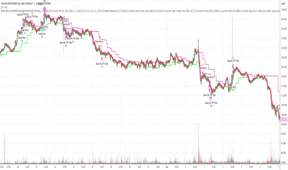
Bober XM v2.0# ₿ober XM v2.0 Trading Bot Documentation
**Developer's Note**: While our previous Bot 1.3.1 was removed due to guideline violations, this setback only fueled our determination to create something even better. Rising from this challenge, Bober XM 2.0 emerges not just as an update, but as a complete reimagining with multi-timeframe analysis, enhanced filters, and superior adaptability. This adversity pushed us to innovate further and deliver a strategy that's smarter, more agile, and more powerful than ever before. Challenges create opportunity - welcome to Cryptobeat's finest work yet.
## !!!!You need to tune it for your own pair and timeframe and retune it periodicaly!!!!!
## Overview
The ₿ober XM v2.0 is an advanced dual-channel trading bot with multi-timeframe analysis capabilities. It integrates multiple technical indicators, customizable risk management, and advanced order execution via webhook for automated trading. The bot's distinctive feature is its separate channel systems for long and short positions, allowing for asymmetric trade strategies that adapt to different market conditions across multiple timeframes.
### Key Features
- **Multi-Timeframe Analysis**: Analyze price data across multiple timeframes simultaneously
- **Dual Channel System**: Separate parameter sets for long and short positions
- **Advanced Entry Filters**: RSI, Volatility, Volume, Bollinger Bands, and KEMAD filters
- **Machine Learning Moving Average**: Adaptive prediction-based channels
- **Multiple Entry Strategies**: Breakout, Pullback, and Mean Reversion modes
- **Risk Management**: Customizable stop-loss, take-profit, and trailing stop settings
- **Webhook Integration**: Compatible with external trading bots and platforms
### Strategy Components
| Component | Description |
|---------|-------------|
| **Dual Channel Trading** | Uses either Keltner Channels or Machine Learning Moving Average (MLMA) with separate settings for long and short positions |
| **MLMA Implementation** | Machine learning algorithm that predicts future price movements and creates adaptive bands |
| **Pivot Point SuperTrend** | Trend identification and confirmation system based on pivot points |
| **Three Entry Strategies** | Choose between Breakout, Pullback, or Mean Reversion approaches |
| **Advanced Filter System** | Multiple customizable filters with multi-timeframe support to avoid false signals |
| **Custom Exit Logic** | Exits based on OBV crossover of its moving average combined with pivot trend changes |
### Note for Novice Users
This is a fully featured real trading bot and can be tweaked for any ticker — SOL is just an example. It follows this structure:
1. **Indicator** – gives the initial signal
2. **Entry strategy** – decides when to open a trade
3. **Exit strategy** – defines when to close it
4. **Trend confirmation** – ensures the trade follows the market direction
5. **Filters** – cuts out noise and avoids weak setups
6. **Risk management** – controls losses and protects your capital
To tune it for a different pair, you'll need to start from scratch:
1. Select the timeframe (candle size)
2. Turn off all filters and trend entry/exit confirmations
3. Choose a channel type, channel source and entry strategy
4. Adjust risk parameters
5. Tune long and short settings for the channel
6. Fine-tune the Pivot Point Supertrend and Main Exit condition OBV
This will generate a lot of signals and activity on the chart. Your next task is to find the right combination of filters and settings to reduce noise and tune it for profitability.
### Default Strategy values
Default values are tuned for: Symbol BITGET:SOLUSDT.P 5min candle
Filters are off by default: Try to play with it to understand how it works
## Configuration Guide
### General Settings
| Setting | Description | Default Value |
|---------|-------------|---------------|
| **Long Positions** | Enable or disable long trades | Enabled |
| **Short Positions** | Enable or disable short trades | Enabled |
| **Risk/Reward Area** | Visual display of stop-loss and take-profit zones | Enabled |
| **Long Entry Source** | Price data used for long entry signals | hl2 (High+Low/2) |
| **Short Entry Source** | Price data used for short entry signals | hl2 (High+Low/2) |
The bot allows you to trade long positions, short positions, or both simultaneously. Each direction has its own set of parameters, allowing for fine-tuned strategies that recognize the asymmetric nature of market movements.
### Multi-Timeframe Settings
1. **Enable Multi-Timeframe Analysis**: Toggle 'Enable Multi-Timeframe Analysis' in the Multi-Timeframe Settings section
2. **Configure Timeframes**: Set appropriate higher timeframes based on your trading style:
- Timeframe 1: Default is now 15 minutes (intraday confirmation)
- Timeframe 2: Default is 4 hours (trend direction)
3. **Select Sources per Indicator**: For each indicator (RSI, KEMAD, Volume, etc.), choose:
- The desired timeframe (current, mtf1, or mtf2)
- The appropriate price type (open, high, low, close, hl2, hlc3, ohlc4)
### Entry Strategies
- **Breakout**: Enter when price breaks above/below the channel
- **Pullback**: Enter when price pulls back to the channel
- **Mean Reversion**: Enter when price is extended from the channel
You can enable different strategies for long and short positions.
### Core Components
### Risk Management
- **Position Size**: Control risk with percentage-based position sizing
- **Stop Loss Options**:
- Fixed: Set a specific price or percentage from entry
- ATR-based: Dynamic stop-loss based on market volatility
- Swing: Uses recent swing high/low points
- **Take Profit**: Multiple targets with percentage allocation
- **Trailing Stop**: Dynamic stop that follows price movement
## Advanced Usage Strategies
### Moving Average Type Selection Guide
- **SMA**: More stable in choppy markets, good for higher timeframes
- **EMA/WMA**: More responsive to recent price changes, better for entry signals
- **VWMA**: Adds volume weighting for stronger trends, use with Volume filter
- **HMA**: Balance between responsiveness and noise reduction, good for volatile markets
### Multi-Timeframe Strategy Approaches
- **Trend Confirmation**: Use higher timeframe RSI (mtf2) for overall trend, current timeframe for entries
- **Entry Precision**: Use KEMAD on current timeframe with volume filter on mtf1
- **False Signal Reduction**: Apply RSI filter on mtf1 with strict KEMAD settings
### Market Condition Optimization
| Market Condition | Recommended Settings |
|------------------|----------------------|
| **Trending** | Use Breakout strategy with KEMAD filter on higher timeframe |
| **Ranging** | Use Mean Reversion with strict RSI filter (mtf1) |
| **Volatile** | Increase ATR multipliers, use HMA for moving averages |
| **Low Volatility** | Decrease noise parameters, use pullback strategy |
## Webhook Integration
The strategy features a professional webhook system that allows direct connectivity to your exchange or trading platform of choice through third-party services like 3commas, Alertatron, or Autoview.
The webhook payload includes all necessary parameters for automated execution:
- Entry price and direction
- Stop loss and take profit levels
- Position size
- Custom identifier for webhook routing
## Performance Optimization Tips
1. **Start with Defaults**: Begin with the default settings for your timeframe before customizing
2. **Adjust One Component at a Time**: Make incremental changes and test the impact
3. **Match MA Types to Market Conditions**: Use appropriate moving average types based on the Market Condition Optimization table
4. **Timeframe Synergy**: Create logical relationships between timeframes (e.g., 5min chart with 15min and 4h higher timeframes)
5. **Periodic Retuning**: Markets evolve - regularly review and adjust parameters
## Common Setups
### Crypto Trend-Following
- MLMA with EMA or HMA
- Higher RSI thresholds (75/25)
- KEMAD filter on mtf1
- Breakout entry strategy
### Stock Swing Trading
- MLMA with SMA for stability
- Volume filter with higher threshold
- KEMAD with increased filter order
- Pullback entry strategy
### Forex Scalping
- MLMA with WMA and lower noise parameter
- RSI filter on current timeframe
- Use highest timeframe for trend direction only
- Mean Reversion strategy
## Webhook Configuration
- **Benefits**:
- Automated trade execution without manual intervention
- Immediate response to market conditions
- Consistent execution of your strategy
- **Implementation Notes**:
- Requires proper webhook configuration on your exchange or platform
- Test thoroughly with small position sizes before full deployment
- Consider latency between signal generation and execution
### Backtesting Period
Define a specific historical period to evaluate the bot's performance:
| Setting | Description | Default Value |
|---------|-------------|---------------|
| **Start Date** | Beginning of backtest period | January 1, 2025 |
| **End Date** | End of backtest period | December 31, 2026 |
- **Best Practice**: Test across different market conditions (bull markets, bear markets, sideways markets)
- **Limitation**: Past performance doesn't guarantee future results
## Entry and Exit Strategies
### Dual-Channel System
A key innovation of the Bober XM is its dual-channel approach:
- **Independent Parameters**: Each trade direction has its own channel settings
- **Asymmetric Trading**: Recognizes that markets often behave differently in uptrends versus downtrends
- **Optimized Performance**: Fine-tune settings for both bullish and bearish conditions
This approach allows the bot to adapt to the natural asymmetry of markets, where uptrends often develop gradually while downtrends can be sharp and sudden.
### Channel Types
#### 1. Keltner Channels
Traditional volatility-based channels using EMA and ATR:
| Setting | Long Default | Short Default |
|---------|--------------|---------------|
| **EMA Length** | 37 | 20 |
| **ATR Length** | 13 | 17 |
| **Multiplier** | 1.4 | 1.9 |
| **Source** | low | high |
- **Strengths**:
- Reliable in trending markets
- Less prone to whipsaws than Bollinger Bands
- Clear visual representation of volatility
- **Weaknesses**:
- Can lag during rapid market changes
- Less effective in choppy, non-trending markets
#### 2. Machine Learning Moving Average (MLMA)
Advanced predictive model using kernel regression (RBF kernel):
| Setting | Description | Options |
|---------|-------------|--------|
| **Source MA** | Price data used for MA calculations | Any price source (low/high/close/etc.) |
| **Moving Average Type** | Type of MA algorithm for calculations | SMA, EMA, WMA, VWMA, RMA, HMA |
| **Trend Source** | Price data used for trend determination | Any price source (close default) |
| **Window Size** | Historical window for MLMA calculations | 5+ (default: 16) |
| **Forecast Length** | Number of bars to forecast ahead | 1+ (default: 3) |
| **Noise Parameter** | Controls smoothness of prediction | 0.01+ (default: ~0.43) |
| **Band Multiplier** | Multiplier for channel width | 0.1+ (default: 0.5-0.6) |
- **Strengths**:
- Predictive rather than reactive
- Adapts quickly to changing market conditions
- Better at identifying trend reversals early
- **Weaknesses**:
- More computationally intensive
- Requires careful parameter tuning
- Can be sensitive to input data quality
### Entry Strategies
| Strategy | Description | Ideal Market Conditions |
|----------|-------------|-------------------------|
| **Breakout** | Enters when price breaks through channel bands, indicating strong momentum | High volatility, emerging trends |
| **Pullback** | Enters when price retraces to the middle band after testing extremes | Established trends with regular pullbacks |
| **Mean Reversion** | Enters at channel extremes, betting on a return to the mean | Range-bound or oscillating markets |
#### Breakout Strategy (Default)
- **Implementation**: Enters long when price crosses above the upper band, short when price crosses below the lower band
- **Strengths**: Captures strong momentum moves, performs well in trending markets
- **Weaknesses**: Can lead to late entries, higher risk of false breakouts
- **Optimization Tips**:
- Increase channel multiplier for fewer but more reliable signals
- Combine with volume confirmation for better accuracy
#### Pullback Strategy
- **Implementation**: Enters long when price pulls back to middle band during uptrend, short during downtrend pullbacks
- **Strengths**: Better entry prices, lower risk, higher probability setups
- **Weaknesses**: Misses some strong moves, requires clear trend identification
- **Optimization Tips**:
- Use with trend filters to confirm overall direction
- Adjust middle band calculation for market volatility
#### Mean Reversion Strategy
- **Implementation**: Enters long at lower band, short at upper band, expecting price to revert to the mean
- **Strengths**: Excellent entry prices, works well in ranging markets
- **Weaknesses**: Dangerous in strong trends, can lead to fighting the trend
- **Optimization Tips**:
- Implement strong trend filters to avoid counter-trend trades
- Use smaller position sizes due to higher risk nature
### Confirmation Indicators
#### Pivot Point SuperTrend
Combines pivot points with ATR-based SuperTrend for trend confirmation:
| Setting | Default Value |
|---------|---------------|
| **Pivot Period** | 25 |
| **ATR Factor** | 2.2 |
| **ATR Period** | 41 |
- **Function**: Identifies significant market turning points and confirms trend direction
- **Implementation**: Requires price to respect the SuperTrend line for trade confirmation
#### Weighted Moving Average (WMA)
Provides additional confirmation layer for entries:
| Setting | Default Value |
|---------|---------------|
| **Period** | 15 |
| **Source** | ohlc4 (average of Open, High, Low, Close) |
- **Function**: Confirms trend direction and filters out low-quality signals
- **Implementation**: Price must be above WMA for longs, below for shorts
### Exit Strategies
#### On-Balance Volume (OBV) Based Exits
Uses volume flow to identify potential reversals:
| Setting | Default Value |
|---------|---------------|
| **Source** | ohlc4 |
| **MA Type** | HMA (Options: SMA, EMA, WMA, RMA, VWMA, HMA) |
| **Period** | 22 |
- **Function**: Identifies divergences between price and volume to exit before reversals
- **Implementation**: Exits when OBV crosses its moving average in the opposite direction
- **Customizable MA Type**: Different MA types provide varying sensitivity to OBV changes:
- **SMA**: Traditional simple average, equal weight to all periods
- **EMA**: More weight to recent data, responds faster to price changes
- **WMA**: Weighted by recency, smoother than EMA
- **RMA**: Similar to EMA but smoother, reduces noise
- **VWMA**: Factors in volume, helpful for OBV confirmation
- **HMA**: Reduces lag while maintaining smoothness (default)
#### ADX Exit Confirmation
Uses Average Directional Index to confirm trend exhaustion:
| Setting | Default Value |
|---------|---------------|
| **ADX Threshold** | 35 |
| **ADX Smoothing** | 60 |
| **DI Length** | 60 |
- **Function**: Confirms trend weakness before exiting positions
- **Implementation**: Requires ADX to drop below threshold or DI lines to cross
## Filter System
### RSI Filter
- **Function**: Controls entries based on momentum conditions
- **Parameters**:
- Period: 15 (default)
- Overbought level: 71
- Oversold level: 23
- Multi-timeframe support: Current, MTF1 (15min), or MTF2 (4h)
- Customizable price source (open, high, low, close, hl2, hlc3, ohlc4)
- **Implementation**: Blocks long entries when RSI > overbought, short entries when RSI < oversold
### Volatility Filter
- **Function**: Prevents trading during excessive market volatility
- **Parameters**:
- Measure: ATR (Average True Range)
- Period: Customizable (default varies by timeframe)
- Threshold: Adjustable multiplier
- Multi-timeframe support
- Customizable price source
- **Implementation**: Blocks trades when current volatility exceeds threshold × average volatility
### Volume Filter
- **Function**: Ensures adequate market liquidity for trades
- **Parameters**:
- Threshold: 0.4× average (default)
- Measurement period: 5 (default)
- Moving average type: Customizable (HMA default)
- Multi-timeframe support
- Customizable price source
- **Implementation**: Requires current volume to exceed threshold × average volume
### Bollinger Bands Filter
- **Function**: Controls entries based on price relative to statistical boundaries
- **Parameters**:
- Period: Customizable
- Standard deviation multiplier: Adjustable
- Moving average type: Customizable
- Multi-timeframe support
- Customizable price source
- **Implementation**: Can require price to be within bands or breaking out of bands depending on strategy
### KEMAD Filter (Kalman EMA Distance)
- **Function**: Advanced trend confirmation using Kalman filter algorithm
- **Parameters**:
- Process Noise: 0.35 (controls smoothness)
- Measurement Noise: 24 (controls reactivity)
- Filter Order: 6 (higher = more smoothing)
- ATR Length: 8 (for bandwidth calculation)
- Upper Multiplier: 2.0 (for long signals)
- Lower Multiplier: 2.7 (for short signals)
- Multi-timeframe support
- Customizable visual indicators
- **Implementation**: Generates signals based on price position relative to Kalman-filtered EMA bands
## Risk Management System
### Position Sizing
Automatically calculates position size based on account equity and risk parameters:
| Setting | Default Value |
|---------|---------------|
| **Risk % of Equity** | 50% |
- **Implementation**:
- Position size = (Account equity × Risk %) ÷ (Entry price × Stop loss distance)
- Adjusts automatically based on volatility and stop placement
- **Best Practices**:
- Start with lower risk percentages (1-2%) until strategy is proven
- Consider reducing risk during high volatility periods
### Stop-Loss Methods
Multiple stop-loss calculation methods with separate configurations for long and short positions:
| Method | Description | Configuration |
|--------|-------------|---------------|
| **ATR-Based** | Dynamic stops based on volatility | ATR Period: 14, Multiplier: 2.0 |
| **Percentage** | Fixed percentage from entry | Long: 1.5%, Short: 1.5% |
| **PIP-Based** | Fixed currency unit distance | 10.0 pips |
- **Implementation Notes**:
- ATR-based stops adapt to changing market volatility
- Percentage stops maintain consistent risk exposure
- PIP-based stops provide precise control in stable markets
### Trailing Stops
Locks in profits by adjusting stop-loss levels as price moves favorably:
| Setting | Default Value |
|---------|---------------|
| **Stop-Loss %** | 1.5% |
| **Activation Threshold** | 2.1% |
| **Trailing Distance** | 1.4% |
- **Implementation**:
- Initial stop remains fixed until profit reaches activation threshold
- Once activated, stop follows price at specified distance
- Locks in profit while allowing room for normal price fluctuations
### Risk-Reward Parameters
Defines the relationship between risk and potential reward:
| Setting | Default Value |
|---------|---------------|
| **Risk-Reward Ratio** | 1.4 |
| **Take Profit %** | 2.4% |
| **Stop-Loss %** | 1.5% |
- **Implementation**:
- Take profit distance = Stop loss distance × Risk-reward ratio
- Higher ratios require fewer winning trades for profitability
- Lower ratios increase win rate but reduce average profit
### Filter Combinations
The strategy allows for simultaneous application of multiple filters:
- **Recommended Combinations**:
- Trending markets: RSI + KEMAD filters
- Ranging markets: Bollinger Bands + Volatility filters
- All markets: Volume filter as minimum requirement
- **Performance Impact**:
- Each additional filter reduces the number of trades
- Quality of remaining trades typically improves
- Optimal combination depends on market conditions and timeframe
### Multi-Timeframe Filter Applications
| Filter Type | Current Timeframe | MTF1 (15min) | MTF2 (4h) |
|-------------|-------------------|-------------|------------|
| RSI | Quick entries/exits | Intraday trend | Overall trend |
| Volume | Immediate liquidity | Sustained support | Market participation |
| Volatility | Entry timing | Short-term risk | Regime changes |
| KEMAD | Precise signals | Trend confirmation | Major reversals |
## Visual Indicators and Chart Analysis
The bot provides comprehensive visual feedback on the chart:
- **Channel Bands**: Keltner or MLMA bands showing potential support/resistance
- **Pivot SuperTrend**: Colored line showing trend direction and potential reversal points
- **Entry/Exit Markers**: Annotations showing actual trade entries and exits
- **Risk/Reward Zones**: Visual representation of stop-loss and take-profit levels
These visual elements allow for:
- Real-time strategy assessment
- Post-trade analysis and optimization
- Educational understanding of the strategy logic
## Implementation Guide
### TradingView Setup
1. Load the script in TradingView Pine Editor
2. Apply to your preferred chart and timeframe
3. Adjust parameters based on your trading preferences
4. Enable alerts for webhook integration
### Webhook Integration
1. Configure webhook URL in TradingView alerts
2. Set up receiving endpoint on your trading platform
3. Define message format matching the bot's output
4. Test with small position sizes before full deployment
### Optimization Process
1. Backtest across different market conditions
2. Identify parameter sensitivity through multiple tests
3. Focus on risk management parameters first
4. Fine-tune entry/exit conditions based on performance metrics
5. Validate with out-of-sample testing
## Performance Considerations
### Strengths
- Adaptability to different market conditions through dual channels
- Multiple layers of confirmation reducing false signals
- Comprehensive risk management protecting capital
- Machine learning integration for predictive edge
### Limitations
- Complex parameter set requiring careful optimization
- Potential over-optimization risk with so many variables
- Computational intensity of MLMA calculations
- Dependency on proper webhook configuration for execution
### Best Practices
- Start with conservative risk settings (1-2% of equity)
- Test thoroughly in demo environment before live trading
- Monitor performance regularly and adjust parameters
- Consider market regime changes when evaluating results
## Conclusion
The ₿ober XM v2.0 represents a significant evolution in trading strategy design, combining traditional technical analysis with machine learning elements and multi-timeframe analysis. The core strength of this system lies in its adaptability and recognition of market asymmetry.
### Market Asymmetry and Adaptive Approach
The strategy acknowledges a fundamental truth about markets: bullish and bearish phases behave differently and should be treated as distinct environments. The dual-channel system with separate parameters for long and short positions directly addresses this asymmetry, allowing for optimized performance regardless of market direction.
### Targeted Backtesting Philosophy
It's counterproductive to run backtests over excessively long periods. Markets evolve continuously, and strategies that worked in previous market regimes may be ineffective in current conditions. Instead:
- Test specific market phases separately (bull markets, bear markets, range-bound periods)
- Regularly re-optimize parameters as market conditions change
- Focus on recent performance with higher weight than historical results
- Test across multiple timeframes to ensure robustness
### Multi-Timeframe Analysis as a Game-Changer
The integration of multi-timeframe analysis fundamentally transforms the strategy's effectiveness:
- **Increased Safety**: Higher timeframe confirmations reduce false signals and improve trade quality
- **Context Awareness**: Decisions made with awareness of larger trends reduce adverse entries
- **Adaptable Precision**: Apply strict filters on lower timeframes while maintaining awareness of broader conditions
- **Reduced Noise**: Higher timeframe data naturally filters market noise that can trigger poor entries
The ₿ober XM v2.0 provides traders with a framework that acknowledges market complexity while offering practical tools to navigate it. With proper setup, realistic expectations, and attention to changing market conditions, it delivers a sophisticated approach to systematic trading that can be continuously refined and optimized.
libHTF[without request.security()]Library "libHTF"
libHTF: use HTF values without request.security()
This library enables to use HTF candles without request.security().
Basic data structure
Using to access values in the same manner as series variable.
The last member of HTF array is always latest current TF's data.
If new bar in HTF(same as last bar closes), new member is pushed to HTF array.
2nd from the last member of HTF array is latest fixed(closed) bar.
HTF: How to use
1. set TF
tf_higher() function selects higher TF. TF steps are ("1","5","15","60","240","D","W","M","3M","6M","Y").
example:
tfChart = timeframe.period
htf1 = tf_higher(tfChart)
2. set HTF matrix
htf_candle() function returns 1 bool and 1 matrix.
bool is a flag for start of new candle in HTF context.
matrix is HTF candle data(0:open,1:time_open,2:close,3:time_close,4:high,5:time:high,6:low,7:time_low).
example:
=htf_candle(htf1)
3. how to access HTF candle data
you can get values using .lastx() method.
please be careful, return value is always float evenif it is "time". you need to cast to int time value when using for xloc.bartime.
example:
htf1open=m1.lastx("open")
htf1close=m1.lastx("close")
//if you need to use histrical value.
lastopen=open
lasthtf1open=m1.lastx("open",1)
4. how to store Data of HTF context
you have to use array to store data of HTF context.
array.htf_push() method handles the last member of array. if new_bar in HTF, it push new member. otherwise it set value to the last member.
example:
array a_close=array.new(1,na)
a_close.htf_push(b_new_bar1,m1.lastx("close"))
HTFsrc: How to use
1. how to setup src.
set_src() function is set current tf's src from string(open/high/low/close/hl2/hlc3/ohlc4/hlcc4).
set_htfsrc() function returns src array of HTF candle.
example:
_src="ohlc4"
src=set_src(_src)
htf1src=set_htfsrc(_src,b_new_bar1,m1)
(if you need to use HTF src in series float)
s_htf1src=htf1src.lastx()
HighLow: How to use
1. set HTF arrays
highlow() and htfhighlow() function calculates high/low and return high/low prices and time.
the functions return 1 int and 8arrays.
int is a flag for new high(1) or new low(-1).
arrays are high/low and return high/low data. float for price, int for time.
example
=
highlow()
=
htfhighlow(m1)
2. how to access HighLow data
you can get values using .lastx() method.
example:
if i_renew==1
myhigh=a_high.lastx()
//if you need to use histrical value.
myhigh=a_high.lastx(1)
other functions
functions for HTF candle matrix or HTF src array in this script are
htf_sma()/htf_ema()/htf_rma()
htf_rsi()/htf_rci()/htf_dmi()
method lastx(arrayid, lastindex)
method like array.last. it returns lastindex from the last member, if parameter is set.
Namespace types: float
Parameters:
arrayid (float )
lastindex (int) : (int) default value is "0"(the last member). if you need to access historical value, increment it(same manner as series vars).
Returns: float value of lastindex from the last member of the array. returns na, if fail.
method lastx(arrayid, lastindex)
method like array.last. it returns lastindex from the last member, if parameter is set.
Namespace types: int
Parameters:
arrayid (int )
lastindex (int) : (int) default value is "0"(the last member). if you need to access historical value, increment it(same manner as series vars).
Returns: int value of lastindex from the last member of the array. returns na, if fail.
method lastx(m, _type, lastindex)
method for handling htf matrix.
Namespace types: matrix
Parameters:
m (matrix) : (matrix) matrix for htf candle.
_type (string) : (string) value type of htf candle:
lastindex (int) : (int) default value is "0"(the last member).
Returns: (float) value of htf candle. (caution: need to cast float to int to use time values!)
method set_last(arrayid, val)
method to set a value of the last member of the array. it sets value to the last member.
Namespace types: float
Parameters:
arrayid (float )
val (float) : (float) value to set.
Returns: nothing
method htf_push(arrayid, b, val)
method to push new member to htf context. if new bar in htf, it works as push. else it works as set_last.
Namespace types: float
Parameters:
arrayid (float )
b (bool) : (bool) true:push,false:set_last
val (float) : (float) _f the value to set.
Returns: nothing
method tf_higher(tf)
method to set higher tf from tf string. TF steps are .
Namespace types: series string, simple string, input string, const string
Parameters:
tf (string) : (string) tf string
Returns: (string) string of higher tf.
htf_candle(_tf, _TZ)
build htf candles
Parameters:
_tf (string) : (string) tf string.
_TZ (string) : of timezone. default value is "GMT+3".
Returns: bool for new bar@htf and matrix for snapshot of htf candle
set_src(_src_type)
set src.
Parameters:
_src_type (string) : (string) type of source:
Returns: (series float) src value
set_htfsrc(_src_type, _nb, _m)
set htf src.
Parameters:
_src_type (string) : (string) type of source:
_nb (bool) : (bool) flag of new bar
_m (matrix) : (matrix) matrix for htf candle.
Returns: (array) array of src value
is_up()
last_is_up()
peak_bottom(_latest, _last)
Parameters:
_latest (bool)
_last (bool)
htf_is_up(_m)
Parameters:
_m (matrix)
htf_last_is_up(_m)
Parameters:
_m (matrix)
highlow(_b_bartime_price)
Parameters:
_b_bartime_price (bool)
htfhighlow(_m, _b_bartime_price)
Parameters:
_m (matrix)
_b_bartime_price (bool)
htf_sma(_a_src, _len)
Parameters:
_a_src (float )
_len (int)
htf_rma(_a_src, _new_bar, _len)
Parameters:
_a_src (float )
_new_bar (bool)
_len (int)
htf_ema(_a_src, _new_bar, _len)
Parameters:
_a_src (float )
_new_bar (bool)
_len (int)
htf_rsi(_a_src, _new_bar, _len)
Parameters:
_a_src (float )
_new_bar (bool)
_len (int)
rci(_src, _len)
Parameters:
_src (float)
_len (int)
htf_rci(_a_src, _len)
Parameters:
_a_src (float )
_len (int)
htf_dmi(_m, _new_bar, _len, _ma_type)
Parameters:
_m (matrix)
_new_bar (bool)
_len (int)
_ma_type (string)

FULL MA Optimization ScriptHello!
This script measures the performance of 10 moving averages and compares them!
Crossover and crossunders are both tested.
The tested moving averages include: TEMA, DEMA, EMA, SMA, ALMA, HMA, T3 Average, WMA, VWMA, LSMA.
You can select the length of the moving averages and the data source (I.E, close, open, ohlc4, etc.) and the script will calculate your selections!
For instance, if you select a length of 32 and a source of ohlc4 for crossovers, the script will assign the ten moving averages that length and data source and compare the performance for ohlc4 crossovers of the 32TEMA, 32DEMA, 32SMA, 32WMA, etc. If you select crossunder, the script will calculate the performance of ohlc4 crossunders of the same moving average lengths.
Moving average performances are listed in descending order (best to worst) and are categorized by tier: Upper-Tier, Mid-Tier, Lower-Tier. The Upper-Tier displays the three best performing averages relative to the MA length and data source, for the asset on the relevant chart timeframe. The Lower-Tier displays the three worst performing averages. The Mid-Tier displays the moving averages whose performance did not achieve a top three spot or a bottom three spot.
Also calculated is the moving average which achieved the highest cumulative gain/loss and the lowest cumulative gain/loss. Any asset and timeframe can be tested; the script recalculates relative to the chart timeframe. I added a "Benchmark Moving Average" free parameter and a "Custom Moving Average" free parameter. The two operate identically; you can set the length and data source of both for quick and simple comparison between differing average lengths and sources.
If "Crossover" is selected, the "(X Candles)" displayed on the tables reflects the average number of sessions the data source remains above a moving average following a crossover. If "Crossunder" is selected, the "(X Candles)" reflects the average number of sessions the data source remains below the moving average following a crossunder.
If "Crossover" is selected, the listed "X%" reflects the average percentage gain/loss following a source crossover of a moving average up until the source crosses back under the moving average. If "Crossunder" is selected, the listed "X%" reflects the average percentage gain/loss following a source crossunder of a moving average up until the source crosses back over the moving average.
If "Crossover" is selected, the listed "X Crosses" reflects the number of instances in which the source crossed over a moving average. If "Crossunder" is selected, the listed "X Crosses" reflects the number of instances in which the source crossed under a moving average.
Additional tooltips and instructions are included should you access the user input menu.
The moving averages can be plotted as a gradient (highest priced MA to lowest priced MA) alongside the best performing moving average. The moving averages can be plotted in full color, light color alongside the best performing average, or not plotted.
This script improves upon a similar script I have released:
I decided not to update the previous script. The previous script calculates crossovers only and, due to being less code intensive, calculates much quicker. If a user is concerned only with price crossovers, not crossunders, the original script is a better option! It's faster, making it the preferable choice!
This script "FULL MA Optimization" calculates crossovers/crossunders and incorporates additional plot styles. I ran into trouble a few times where the script was too large to run on TV. This script is not "slow", I suppose; however, calculations and parameter modifications take a bit longer than the original script!

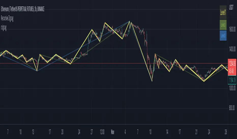
rzigzagLibrary "rzigzag"
Recursive Zigzag Using Matrix allows to create zigzags recursively on multiple levels. This is an old library converted to V6
zigzag(length, ohlc, numberOfPivots, offset)
calculates plain zigzag based on input
Parameters:
length (int) : Zigzag Length
ohlc (array) : Array containing ohlc values. Can also contain custom series
numberOfPivots (simple int) : Number of max pivots to be returned
offset (simple int) : Offset from current bar. Can be used for calculations based on confirmed bars
Returns: [matrix zigzagmatrix, bool flags]
iZigzag(length, h, l, numberOfPivots)
calculates plain zigzag based on input array
Parameters:
length (int) : Zigzag Length
h (array) : array containing high values of a series
l (array) : array containing low values of a series
numberOfPivots (simple int) : Number of max pivots to be returned
Returns: matrix zigzagmatrix
nextlevel(zigzagmatrix, numberOfPivots)
calculates next level zigzag based on present zigzag coordinates
Parameters:
zigzagmatrix (matrix) : Matrix containing zigzag pivots, bars, bar time, direction and level
numberOfPivots (simple int) : Number of max pivots to be returned
Returns: matrix zigzagmatrix
draw(zigzagmatrix, flags, lineColor, lineWidth, lineStyle, showLabel, xloc)
draws zigzag based on the zigzagmatrix input
Parameters:
zigzagmatrix (matrix) : Matrix containing zigzag pivots, bars, bar time, direction and level
flags (array) : Zigzag pivot flags
lineColor (color) : Zigzag line color
lineWidth (int) : Zigzag line width
lineStyle (string) : Zigzag line style
showLabel (bool) : Flag to indicate display pivot labels
xloc (string) : xloc preference for drawing lines/labels
Returns:
draw(length, ohlc, numberOfPivots, offset, lineColor, lineWidth, lineStyle, showLabel, xloc)
calculates and draws zigzag based on zigzag length and source input
Parameters:
length (int) : Zigzag Length
ohlc (array) : Array containing ohlc values. Can also contain custom series
numberOfPivots (simple int) : Number of max pivots to be returned
offset (simple int) : Offset from current bar. Can be used for calculations based on confirmed bars
lineColor (color) : Zigzag line color
lineWidth (int) : Zigzag line width
lineStyle (string) : Zigzag line style
showLabel (bool) : Flag to indicate display pivot labels
xloc (string) : xloc preference for drawing lines/labels
Returns: [matrix zigzagmatrix, array zigzaglines, array zigzaglabels, bool flags]
drawfresh(zigzagmatrix, zigzaglines, zigzaglabels, lineColor, lineWidth, lineStyle, showLabel, xloc)
draws fresh zigzag for all pivots in the input matrix.
Parameters:
zigzagmatrix (matrix) : Matrix containing zigzag pivots, bars, bar time, direction and level
zigzaglines (array) : array to which all newly created lines will be added
zigzaglabels (array) : array to which all newly created lables will be added
lineColor (color) : Zigzag line color
lineWidth (int) : Zigzag line width
lineStyle (string) : Zigzag line style
showLabel (bool) : Flag to indicate display pivot labels
xloc (string) : xloc preference for drawing lines/labels
Returns:

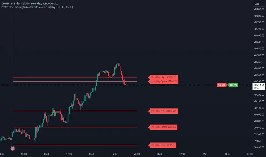
MultiTFlevels with Volume Display1. Overview
This indicator is intended for use on trading platforms like TradingView and provides the following features:
Volume Profile Analysis:
Shows cumulative volume delta (CVD) and displays buying and selling volumes.
Historical OHLC Levels:
Plots historical open, high, low, and close levels for various timeframes (e.g., daily, weekly, monthly).
Customizable Settings:
Allows users to toggle different elements and customize display options.
2. Inputs
Timeframe Display Toggles:
Users can choose to display OHLC levels from different timeframes such as previous month, week, day, 4H, 1H, 30M, 15M, and 5M.
CVD Display Toggle: Option to show or hide the Cumulative Volume Delta (CVD).
Line and Label Customization:
leftOffset and rightOffset: Define how far lines are extended left and right from the current bar.
colorMonth, colorWeek, etc.: Customize colors for different timeframe OHLC levels.
labelOffset and rightOffset: Control the positioning of volume labels.
3. Key Features
Cumulative Volume Delta (CVD)
Calculation:
Computes the cumulative volume delta by adding or subtracting the volume based on whether the close price is higher or lower than the open price.
Display:
Shows a label on the chart indicating the current CVD value and whether the market is leaning towards buying or selling.
Historical OHLC Levels
Data Retrieval:
Uses the request.security function to fetch OHLC data from different timeframes (e.g., monthly, weekly, daily).
Plotting:
Draws lines and labels on the chart to represent open, high, low, and close levels for each selected timeframe.
Buying and Selling Volumes
Calculation:
Calculates buying and selling volumes based on whether the close price is higher or lower than the open price.
Display:
Shows labels on the chart for buying and selling volumes.
4. Functions
getOHLC(timeframe)
Retrieves open, high, low, and close values from the specified timeframe.
plotOHLC(show, open, high, low, close, col, prefix)
Draws OHLC lines and labels on the chart for the given timeframe and color.
5. Usage
Chart Overlay: The indicator is overlaid on the main chart (i.e., it appears directly on the price chart).
Historical Analysis:
Useful for analyzing historical price levels and volume dynamics across different timeframes.
Volume Insights:
Helps traders understand the cumulative volume behavior and market sentiment through the CVD and volume labels.
In essence, this indicator provides a comprehensive view of historical price levels across multiple timeframes and the dynamics of market volume through CVD and volume labels. It can be particularly useful for traders looking to combine price action with volume analysis for a more in-depth market assessment.
rzigzagLibrary "rzigzag"
Recursive Zigzag Using Matrix allows to create zigzags recursively on multiple levels. After bit of consideration, decided to make this public.
zigzag(length, ohlc, numberOfPivots, offset)
calculates plain zigzag based on input
Parameters:
length : Zigzag Length
ohlc : Array containing ohlc values. Can also contain custom series
numberOfPivots : Number of max pivots to be returned
offset : Offset from current bar. Can be used for calculations based on confirmed bars
Returns:
nextlevel(zigzagmatrix, numberOfPivots)
calculates next level zigzag based on present zigzag coordinates
Parameters:
zigzagmatrix : Matrix containing zigzag pivots, bars, bar time, direction and level
numberOfPivots : Number of max pivots to be returned
Returns: matrix zigzagmatrix
draw(zigzagmatrix, newPivot, doublePivot, lineColor, lineWidth, lineStyle, showLabel, xloc)
draws zigzag based on the zigzagmatrix input
Parameters:
zigzagmatrix : Matrix containing zigzag pivots, bars, bar time, direction and level
newPivot : Flag indicating there is update in the pivots
doublePivot : Flag containing there is double pivot update on same bar
lineColor : Zigzag line color
lineWidth : Zigzag line width
lineStyle : Zigzag line style
showLabel : Flag to indicate display pivot labels
xloc : xloc preference for drawing lines/labels
Returns:
draw(length, ohlc, numberOfPivots, offset, lineColor, lineWidth, lineStyle, showLabel, xloc)
calculates and draws zigzag based on zigzag length and source input
Parameters:
length : Zigzag Length
ohlc : Array containing ohlc values. Can also contain custom series
numberOfPivots : Number of max pivots to be returned
offset : Offset from current bar. Can be used for calculations based on confirmed bars
lineColor : Zigzag line color
lineWidth : Zigzag line width
lineStyle : Zigzag line style
showLabel : Flag to indicate display pivot labels
xloc : xloc preference for drawing lines/labels
Returns:
drawfresh(zigzagmatrix, zigzaglines, zigzaglabels, lineColor, lineWidth, lineStyle, showLabel, xloc)
draws fresh zigzag for all pivots in the input matrix.
Parameters:
zigzagmatrix : Matrix containing zigzag pivots, bars, bar time, direction and level
zigzaglines : array to which all newly created lines will be added
zigzaglabels : array to which all newly created lables will be added
lineColor : Zigzag line color
lineWidth : Zigzag line width
lineStyle : Zigzag line style
showLabel : Flag to indicate display pivot labels
xloc : xloc preference for drawing lines/labels
Returns:
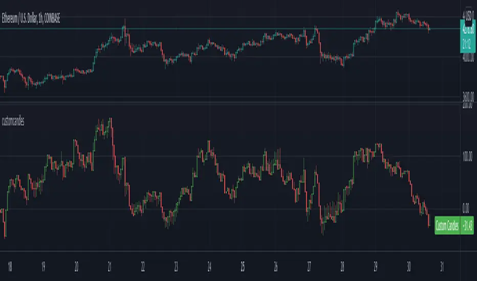
customcandlesLibrary "customcandles"
customcandles: Contains methods which can send custom candlesticks based on the input
macandles(maType, length, o, h, l, c) macandles: Provides OHLC of moving average candles
Parameters:
maType : - Moving average Type. Can be sma, ema, hma, rma, wma, vwma, swma, linreg, median
length : - Defaulted to 20. Can chose custom length
o : - Optional different open source. By default is set to open
h : - Optional different high source. By default is set to high
l : - Optional different low source. By default is set to low
c : - Optional different close source. By default is set to close
Returns: : Custom Moving Average based OHLC values
hacandles() hacandles: Provides Heikin Ashi OHLC values
Returns: : Custom Heikin Ashi OHLC values
ocandles(type, length, shortLength, longLength, method, highlowLength, sticky, percentCandles) macandles: Provides OHLC of moving average candles
Parameters:
type : - Oscillator Type. Can be cci, cmo, cog, mfi, roc, rsi, tsi, mfi
length : - Defaulted to 14. Can chose custom length
shortLength : - Used only for TSI. Default is 13
longLength : - Used only for TSI. Default is 25
method : - Valid values for method are : sma, ema, hma, rma, wma, vwma, swma, highlow, linreg, median
highlowLength : - length on which highlow of the oscillator is calculated
sticky : - overbought, oversold levels won't change unless crossed
percentCandles : - candles are generated based on percent with respect to high/low instead of actual oscillator values
Returns: : Custom Moving Average based OHLC values
real_time_candlesIntroduction
The Real-Time Candles Library provides comprehensive tools for creating, manipulating, and visualizing custom timeframe candles in Pine Script. Unlike standard indicators that only update at bar close, this library enables real-time visualization of price action and indicators within the current bar, offering traders unprecedented insight into market dynamics as they unfold.
This library addresses a fundamental limitation in traditional technical analysis: the inability to see how indicators evolve between bar closes. By implementing sophisticated real-time data processing techniques, traders can now observe indicator movements, divergences, and trend changes as they develop, potentially identifying trading opportunities much earlier than with conventional approaches.
Key Features
The library supports two primary candle generation approaches:
Chart-Time Candles: Generate real-time OHLC data for any variable (like RSI, MACD, etc.) while maintaining synchronization with chart bars.
Custom Timeframe (CTF) Candles: Create candles with custom time intervals or tick counts completely independent of the chart's native timeframe.
Both approaches support traditional candlestick and Heikin-Ashi visualization styles, with options for moving average overlays to smooth the data.
Configuration Requirements
For optimal performance with this library:
Set max_bars_back = 5000 in your script settings
When using CTF drawing functions, set max_lines_count = 500, max_boxes_count = 500, and max_labels_count = 500
These settings ensure that you will be able to draw correctly and will avoid any runtime errors.
Usage Examples
Basic Chart-Time Candle Visualization
// Create real-time candles for RSI
float rsi = ta.rsi(close, 14)
Candle rsi_candle = candle_series(rsi, CandleType.candlestick)
// Plot the candles using Pine's built-in function
plotcandle(rsi_candle.Open, rsi_candle.High, rsi_candle.Low, rsi_candle.Close,
"RSI Candles", rsi_candle.candle_color, rsi_candle.candle_color)
Multiple Access Patterns
The library provides three ways to access candle data, accommodating different programming styles:
// 1. Array-based access for collection operations
Candle candles = candle_array(source)
// 2. Object-oriented access for single entity manipulation
Candle candle = candle_series(source)
float value = candle.source(Source.HLC3)
// 3. Tuple-based access for functional programming styles
= candle_tuple(source)
Custom Timeframe Examples
// Create 20-second candles with EMA overlay
plot_ctf_candles(
source = close,
candle_type = CandleType.candlestick,
sample_type = SampleType.Time,
number_of_seconds = 20,
timezone = -5,
tied_open = true,
ema_period = 9,
enable_ema = true
)
// Create tick-based candles (new candle every 15 ticks)
plot_ctf_tick_candles(
source = close,
candle_type = CandleType.heikin_ashi,
number_of_ticks = 15,
timezone = -5,
tied_open = true
)
Advanced Usage with Custom Visualization
// Get custom timeframe candles without automatic plotting
CandleCTF my_candles = ctf_candles_array(
source = close,
candle_type = CandleType.candlestick,
sample_type = SampleType.Time,
number_of_seconds = 30
)
// Apply custom logic to the candles
float ema_values = my_candles.ctf_ema(14)
// Draw candles and EMA using time-based coordinates
my_candles.draw_ctf_candles_time()
ema_values.draw_ctf_line_time(line_color = #FF6D00)
Library Components
Data Types
Candle: Structure representing chart-time candles with OHLC, polarity, and visualization properties
CandleCTF: Extended candle structure with additional time metadata for custom timeframes
TickData: Structure for individual price updates with time deltas
Enumerations
CandleType: Specifies visualization style (candlestick or Heikin-Ashi)
Source: Defines price components for calculations (Open, High, Low, Close, HL2, etc.)
SampleType: Sets sampling method (Time-based or Tick-based)
Core Functions
get_tick(): Captures current price as a tick data point
candle_array(): Creates an array of candles from price updates
candle_series(): Provides a single candle based on latest data
candle_tuple(): Returns OHLC values as a tuple
ctf_candles_array(): Creates custom timeframe candles without rendering
Visualization Functions
source(): Extracts specific price components from candles
candle_ctf_to_float(): Converts candle data to float arrays
ctf_ema(): Calculates exponential moving averages for candle arrays
draw_ctf_candles_time(): Renders candles using time coordinates
draw_ctf_candles_index(): Renders candles using bar index coordinates
draw_ctf_line_time(): Renders lines using time coordinates
draw_ctf_line_index(): Renders lines using bar index coordinates
Technical Implementation Notes
This library leverages Pine Script's varip variables for state management, creating a sophisticated real-time data processing system. The implementation includes:
Efficient tick capturing: Samples price at every execution, maintaining temporal tracking with time deltas
Smart state management: Uses a hybrid approach with mutable updates at index 0 and historical preservation at index 1+
Temporal synchronization: Manages two time domains (chart time and custom timeframe)
The tooltip implementation provides crucial temporal context for custom timeframe visualizations, allowing users to understand exactly when each candle formed regardless of chart timeframe.
Limitations
Custom timeframe candles cannot be backtested due to Pine Script's limitations with historical tick data
Real-time visualization is only available during live chart updates
Maximum history is constrained by Pine Script's array size limits
Applications
Indicator visualization: See how RSI, MACD, or other indicators evolve in real-time
Volume analysis: Create custom volume profiles independent of chart timeframe
Scalping strategies: Identify short-term patterns with precisely defined time windows
Volatility measurement: Track price movement characteristics within bars
Custom signal generation: Create entry/exit signals based on custom timeframe patterns
Conclusion
The Real-Time Candles Library bridges the gap between traditional technical analysis (based on discrete OHLC bars) and the continuous nature of market movement. By making indicators more responsive to real-time price action, it gives traders a significant edge in timing and decision-making, particularly in fast-moving markets where waiting for bar close could mean missing important opportunities.
Whether you're building custom indicators, researching price patterns, or developing trading strategies, this library provides the foundation for sophisticated real-time analysis in Pine Script.
Implementation Details & Advanced Guide
Core Implementation Concepts
The Real-Time Candles Library implements a sophisticated event-driven architecture within Pine Script's constraints. At its heart, the library creates what's essentially a reactive programming framework handling continuous data streams.
Tick Processing System
The foundation of the library is the get_tick() function, which captures price updates as they occur:
export get_tick(series float source = close, series float na_replace = na)=>
varip float price = na
varip int series_index = -1
varip int old_time = 0
varip int new_time = na
varip float time_delta = 0
// ...
This function:
Samples the current price
Calculates time elapsed since last update
Maintains a sequential index to track updates
The resulting TickData structure serves as the fundamental building block for all candle generation.
State Management Architecture
The library employs a sophisticated state management system using varip variables, which persist across executions within the same bar. This creates a hybrid programming paradigm that's different from standard Pine Script's bar-by-bar model.
For chart-time candles, the core state transition logic is:
// Real-time update of current candle
candle_data := Candle.new(Open, High, Low, Close, polarity, series_index, candle_color)
candles.set(0, candle_data)
// When a new bar starts, preserve the previous candle
if clear_state
candles.insert(1, candle_data)
price.clear()
// Reset state for new candle
Open := Close
price.push(Open)
series_index += 1
This pattern of updating index 0 in real-time while inserting completed candles at index 1 creates an elegant solution for maintaining both current state and historical data.
Custom Timeframe Implementation
The custom timeframe system manages its own time boundaries independent of chart bars:
bool clear_state = switch settings.sample_type
SampleType.Ticks => cumulative_series_idx >= settings.number_of_ticks
SampleType.Time => cumulative_time_delta >= settings.number_of_seconds
This dual-clock system synchronizes two time domains:
Pine's execution clock (bar-by-bar processing)
The custom timeframe clock (tick or time-based)
The library carefully handles temporal discontinuities, ensuring candle formation remains accurate despite irregular tick arrival or market gaps.
Advanced Usage Techniques
1. Creating Custom Indicators with Real-Time Candles
To develop indicators that process real-time data within the current bar:
// Get real-time candles for your data
Candle rsi_candles = candle_array(ta.rsi(close, 14))
// Calculate indicator values based on candle properties
float signal = ta.ema(rsi_candles.first().source(Source.Close), 9)
// Detect patterns that occur within the bar
bool divergence = close > close and rsi_candles.first().Close < rsi_candles.get(1).Close
2. Working with Custom Timeframes and Plotting
For maximum flexibility when visualizing custom timeframe data:
// Create custom timeframe candles
CandleCTF volume_candles = ctf_candles_array(
source = volume,
candle_type = CandleType.candlestick,
sample_type = SampleType.Time,
number_of_seconds = 60
)
// Convert specific candle properties to float arrays
float volume_closes = volume_candles.candle_ctf_to_float(Source.Close)
// Calculate derived values
float volume_ema = volume_candles.ctf_ema(14)
// Create custom visualization
volume_candles.draw_ctf_candles_time()
volume_ema.draw_ctf_line_time(line_color = color.orange)
3. Creating Hybrid Timeframe Analysis
One powerful application is comparing indicators across multiple timeframes:
// Standard chart timeframe RSI
float chart_rsi = ta.rsi(close, 14)
// Custom 5-second timeframe RSI
CandleCTF ctf_candles = ctf_candles_array(
source = close,
candle_type = CandleType.candlestick,
sample_type = SampleType.Time,
number_of_seconds = 5
)
float fast_rsi_array = ctf_candles.candle_ctf_to_float(Source.Close)
float fast_rsi = fast_rsi_array.first()
// Generate signals based on divergence between timeframes
bool entry_signal = chart_rsi < 30 and fast_rsi > fast_rsi_array.get(1)
Final Notes
This library represents an advanced implementation of real-time data processing within Pine Script's constraints. By creating a reactive programming framework for handling continuous data streams, it enables sophisticated analysis typically only available in dedicated trading platforms.
The design principles employed—including state management, temporal processing, and object-oriented architecture—can serve as patterns for other advanced Pine Script development beyond this specific application.
------------------------
Library "real_time_candles"
A comprehensive library for creating real-time candles with customizable timeframes and sampling methods.
Supports both chart-time and custom-time candles with options for candlestick and Heikin-Ashi visualization.
Allows for tick-based or time-based sampling with moving average overlay capabilities.
get_tick(source, na_replace)
Captures the current price as a tick data point
Parameters:
source (float) : Optional - Price source to sample (defaults to close)
na_replace (float) : Optional - Value to use when source is na
Returns: TickData structure containing price, time since last update, and sequential index
candle_array(source, candle_type, sync_start, bullish_color, bearish_color)
Creates an array of candles based on price updates
Parameters:
source (float) : Optional - Price source to sample (defaults to close)
candle_type (simple CandleType) : Optional - Type of candle chart to create (candlestick or Heikin-Ashi)
sync_start (simple bool) : Optional - Whether to synchronize with the start of a new bar
bullish_color (color) : Optional - Color for bullish candles
bearish_color (color) : Optional - Color for bearish candles
Returns: Array of Candle objects ordered with most recent at index 0
candle_series(source, candle_type, wait_for_sync, bullish_color, bearish_color)
Provides a single candle based on the latest price data
Parameters:
source (float) : Optional - Price source to sample (defaults to close)
candle_type (simple CandleType) : Optional - Type of candle chart to create (candlestick or Heikin-Ashi)
wait_for_sync (simple bool) : Optional - Whether to wait for a new bar before starting
bullish_color (color) : Optional - Color for bullish candles
bearish_color (color) : Optional - Color for bearish candles
Returns: A single Candle object representing the current state
candle_tuple(source, candle_type, wait_for_sync, bullish_color, bearish_color)
Provides candle data as a tuple of OHLC values
Parameters:
source (float) : Optional - Price source to sample (defaults to close)
candle_type (simple CandleType) : Optional - Type of candle chart to create (candlestick or Heikin-Ashi)
wait_for_sync (simple bool) : Optional - Whether to wait for a new bar before starting
bullish_color (color) : Optional - Color for bullish candles
bearish_color (color) : Optional - Color for bearish candles
Returns: Tuple representing current candle values
method source(self, source, na_replace)
Extracts a specific price component from a Candle
Namespace types: Candle
Parameters:
self (Candle)
source (series Source) : Type of price data to extract (Open, High, Low, Close, or composite values)
na_replace (float) : Optional - Value to use when source value is na
Returns: The requested price value from the candle
method source(self, source)
Extracts a specific price component from a CandleCTF
Namespace types: CandleCTF
Parameters:
self (CandleCTF)
source (simple Source) : Type of price data to extract (Open, High, Low, Close, or composite values)
Returns: The requested price value from the candle as a varip
method candle_ctf_to_float(self, source)
Converts a specific price component from each CandleCTF to a float array
Namespace types: array
Parameters:
self (array)
source (simple Source) : Optional - Type of price data to extract (defaults to Close)
Returns: Array of float values extracted from the candles, ordered with most recent at index 0
method ctf_ema(self, ema_period)
Calculates an Exponential Moving Average for a CandleCTF array
Namespace types: array
Parameters:
self (array)
ema_period (simple float) : Period for the EMA calculation
Returns: Array of float values representing the EMA of the candle data, ordered with most recent at index 0
method draw_ctf_candles_time(self, sample_type, number_of_ticks, number_of_seconds, timezone)
Renders custom timeframe candles using bar time coordinates
Namespace types: array
Parameters:
self (array)
sample_type (simple SampleType) : Optional - Method for sampling data (Time or Ticks), used for tooltips
number_of_ticks (simple int) : Optional - Number of ticks per candle (used when sample_type is Ticks), used for tooltips
number_of_seconds (simple float) : Optional - Time duration per candle in seconds (used when sample_type is Time), used for tooltips
timezone (simple int) : Optional - Timezone offset from UTC (-12 to +12), used for tooltips
Returns: void - Renders candles on the chart using time-based x-coordinates
method draw_ctf_candles_index(self, sample_type, number_of_ticks, number_of_seconds, timezone)
Renders custom timeframe candles using bar index coordinates
Namespace types: array
Parameters:
self (array)
sample_type (simple SampleType) : Optional - Method for sampling data (Time or Ticks), used for tooltips
number_of_ticks (simple int) : Optional - Number of ticks per candle (used when sample_type is Ticks), used for tooltips
number_of_seconds (simple float) : Optional - Time duration per candle in seconds (used when sample_type is Time), used for tooltips
timezone (simple int) : Optional - Timezone offset from UTC (-12 to +12), used for tooltips
Returns: void - Renders candles on the chart using index-based x-coordinates
method draw_ctf_line_time(self, source, line_size, line_color)
Renders a line representing a price component from the candles using time coordinates
Namespace types: array
Parameters:
self (array)
source (simple Source) : Optional - Type of price data to extract (defaults to Close)
line_size (simple int) : Optional - Width of the line
line_color (simple color) : Optional - Color of the line
Returns: void - Renders a connected line on the chart using time-based x-coordinates
method draw_ctf_line_time(self, line_size, line_color)
Renders a line from a varip float array using time coordinates
Namespace types: array
Parameters:
self (array)
line_size (simple int) : Optional - Width of the line, defaults to 2
line_color (simple color) : Optional - Color of the line
Returns: void - Renders a connected line on the chart using time-based x-coordinates
method draw_ctf_line_index(self, source, line_size, line_color)
Renders a line representing a price component from the candles using index coordinates
Namespace types: array
Parameters:
self (array)
source (simple Source) : Optional - Type of price data to extract (defaults to Close)
line_size (simple int) : Optional - Width of the line
line_color (simple color) : Optional - Color of the line
Returns: void - Renders a connected line on the chart using index-based x-coordinates
method draw_ctf_line_index(self, line_size, line_color)
Renders a line from a varip float array using index coordinates
Namespace types: array
Parameters:
self (array)
line_size (simple int) : Optional - Width of the line, defaults to 2
line_color (simple color) : Optional - Color of the line
Returns: void - Renders a connected line on the chart using index-based x-coordinates
plot_ctf_tick_candles(source, candle_type, number_of_ticks, timezone, tied_open, ema_period, bullish_color, bearish_color, line_width, ema_color, use_time_indexing)
Plots tick-based candles with moving average
Parameters:
source (float) : Input price source to sample
candle_type (simple CandleType) : Type of candle chart to display
number_of_ticks (simple int) : Number of ticks per candle
timezone (simple int) : Timezone offset from UTC (-12 to +12)
tied_open (simple bool) : Whether to tie open price to close of previous candle
ema_period (simple float) : Period for the exponential moving average
bullish_color (color) : Optional - Color for bullish candles
bearish_color (color) : Optional - Color for bearish candles
line_width (simple int) : Optional - Width of the moving average line, defaults to 2
ema_color (color) : Optional - Color of the moving average line
use_time_indexing (simple bool) : Optional - When true the function will plot with xloc.time, when false it will plot using xloc.bar_index
Returns: void - Creates visual candle chart with EMA overlay
plot_ctf_tick_candles(source, candle_type, number_of_ticks, timezone, tied_open, bullish_color, bearish_color, use_time_indexing)
Plots tick-based candles without moving average
Parameters:
source (float) : Input price source to sample
candle_type (simple CandleType) : Type of candle chart to display
number_of_ticks (simple int) : Number of ticks per candle
timezone (simple int) : Timezone offset from UTC (-12 to +12)
tied_open (simple bool) : Whether to tie open price to close of previous candle
bullish_color (color) : Optional - Color for bullish candles
bearish_color (color) : Optional - Color for bearish candles
use_time_indexing (simple bool) : Optional - When true the function will plot with xloc.time, when false it will plot using xloc.bar_index
Returns: void - Creates visual candle chart without moving average
plot_ctf_time_candles(source, candle_type, number_of_seconds, timezone, tied_open, ema_period, bullish_color, bearish_color, line_width, ema_color, use_time_indexing)
Plots time-based candles with moving average
Parameters:
source (float) : Input price source to sample
candle_type (simple CandleType) : Type of candle chart to display
number_of_seconds (simple float) : Time duration per candle in seconds
timezone (simple int) : Timezone offset from UTC (-12 to +12)
tied_open (simple bool) : Whether to tie open price to close of previous candle
ema_period (simple float) : Period for the exponential moving average
bullish_color (color) : Optional - Color for bullish candles
bearish_color (color) : Optional - Color for bearish candles
line_width (simple int) : Optional - Width of the moving average line, defaults to 2
ema_color (color) : Optional - Color of the moving average line
use_time_indexing (simple bool) : Optional - When true the function will plot with xloc.time, when false it will plot using xloc.bar_index
Returns: void - Creates visual candle chart with EMA overlay
plot_ctf_time_candles(source, candle_type, number_of_seconds, timezone, tied_open, bullish_color, bearish_color, use_time_indexing)
Plots time-based candles without moving average
Parameters:
source (float) : Input price source to sample
candle_type (simple CandleType) : Type of candle chart to display
number_of_seconds (simple float) : Time duration per candle in seconds
timezone (simple int) : Timezone offset from UTC (-12 to +12)
tied_open (simple bool) : Whether to tie open price to close of previous candle
bullish_color (color) : Optional - Color for bullish candles
bearish_color (color) : Optional - Color for bearish candles
use_time_indexing (simple bool) : Optional - When true the function will plot with xloc.time, when false it will plot using xloc.bar_index
Returns: void - Creates visual candle chart without moving average
plot_ctf_candles(source, candle_type, sample_type, number_of_ticks, number_of_seconds, timezone, tied_open, ema_period, bullish_color, bearish_color, enable_ema, line_width, ema_color, use_time_indexing)
Unified function for plotting candles with comprehensive options
Parameters:
source (float) : Input price source to sample
candle_type (simple CandleType) : Optional - Type of candle chart to display
sample_type (simple SampleType) : Optional - Method for sampling data (Time or Ticks)
number_of_ticks (simple int) : Optional - Number of ticks per candle (used when sample_type is Ticks)
number_of_seconds (simple float) : Optional - Time duration per candle in seconds (used when sample_type is Time)
timezone (simple int) : Optional - Timezone offset from UTC (-12 to +12)
tied_open (simple bool) : Optional - Whether to tie open price to close of previous candle
ema_period (simple float) : Optional - Period for the exponential moving average
bullish_color (color) : Optional - Color for bullish candles
bearish_color (color) : Optional - Color for bearish candles
enable_ema (bool) : Optional - Whether to display the EMA overlay
line_width (simple int) : Optional - Width of the moving average line, defaults to 2
ema_color (color) : Optional - Color of the moving average line
use_time_indexing (simple bool) : Optional - When true the function will plot with xloc.time, when false it will plot using xloc.bar_index
Returns: void - Creates visual candle chart with optional EMA overlay
ctf_candles_array(source, candle_type, sample_type, number_of_ticks, number_of_seconds, tied_open, bullish_color, bearish_color)
Creates an array of custom timeframe candles without rendering them
Parameters:
source (float) : Input price source to sample
candle_type (simple CandleType) : Type of candle chart to create (candlestick or Heikin-Ashi)
sample_type (simple SampleType) : Method for sampling data (Time or Ticks)
number_of_ticks (simple int) : Optional - Number of ticks per candle (used when sample_type is Ticks)
number_of_seconds (simple float) : Optional - Time duration per candle in seconds (used when sample_type is Time)
tied_open (simple bool) : Optional - Whether to tie open price to close of previous candle
bullish_color (color) : Optional - Color for bullish candles
bearish_color (color) : Optional - Color for bearish candles
Returns: Array of CandleCTF objects ordered with most recent at index 0
Candle
Structure representing a complete candle with price data and display properties
Fields:
Open (series float) : Opening price of the candle
High (series float) : Highest price of the candle
Low (series float) : Lowest price of the candle
Close (series float) : Closing price of the candle
polarity (series bool) : Boolean indicating if candle is bullish (true) or bearish (false)
series_index (series int) : Sequential index identifying the candle in the series
candle_color (series color) : Color to use when rendering the candle
ready (series bool) : Boolean indicating if candle data is valid and ready for use
TickData
Structure for storing individual price updates
Fields:
price (series float) : The price value at this tick
time_delta (series float) : Time elapsed since the previous tick in milliseconds
series_index (series int) : Sequential index identifying this tick
CandleCTF
Structure representing a custom timeframe candle with additional time metadata
Fields:
Open (series float) : Opening price of the candle
High (series float) : Highest price of the candle
Low (series float) : Lowest price of the candle
Close (series float) : Closing price of the candle
polarity (series bool) : Boolean indicating if candle is bullish (true) or bearish (false)
series_index (series int) : Sequential index identifying the candle in the series
open_time (series int) : Timestamp marking when the candle was opened (in Unix time)
time_delta (series float) : Duration of the candle in milliseconds
candle_color (series color) : Color to use when rendering the candle

Time Based 3 Candle Model CRT FrameworkThe 3 Candle Model Overview:
The 3 Candle Model serves as a sophisticated framework for traders to navigate the complexities of financial markets, particularly within futures and forex trading. This guide not only elaborates on the model's key features but also emphasizes its originality and practical usefulness in the TradingView community. The core principle of the 3 Candle Model revolves around understanding how candle patterns can represent significant price ranges, offering valuable insights into potential market movements. By integrating the model with other critical trading concepts such as the Power of Three (PO3), Open-High-Low-Close (OHLC), and Turtle Soup setups, traders can enhance their ability to identify high-probability trades and achieve better trading outcomes.
Indicator includes:
3 Customizable Timeframe choices to fractally frame 3 candle models for precision
Live Timers for each timeframe to always be aware of the models timing
Parent Candle tracking on every preffered timeframe until new models parent candle is printed
Key Features of the 3 Candle Model
The 3 Candle Model primarily utilizes a three-candle structure, where the first candle establishes a price range, the second candle may act as a confirmation (often termed a "turtle soup"), and the third candle provides the breakout or continuation. This structure is pivotal in determining entry and exit points for trades, ensuring that each trading decision is backed by solid price action analysis.
OHLC Principle:
The Open-High-Low-Close (OHLC) concept is integral to the 3 Candle Model, allowing traders to analyze price action more effectively. Understanding the relationship between these four price points helps traders gauge market sentiment and potential reversals. By incorporating OHLC into the model, traders can develop a deeper understanding of market structure and its implications for future price movements.
Delivery States:
The 3 Candle Model emphasizes the importance of delivery states, which refer to the market's phase during specific time frames. Recognizing these states aids traders in determining the appropriate conditions for entering trades, particularly when combined with the power of three and candle range patterns. This understanding is crucial for positioning trades in alignment with market momentum.
High Probability Setups:
By aligning the 3 Candle Model with inside bar setups, traders can optimize their strategies for high-probability outcomes. This approach capitalizes on the inherent fractal nature of price movements, where previous patterns repeat at different scales. The combination of the model and inside bar setups enhances the trader's toolkit, allowing for more strategic trade placements.
Turtle Soup Formation:
The 3 Candle Model intricately connects with the Turtle Soup concept, which focuses on false breakouts. Identifying these formations at critical levels enhances the trader's ability to anticipate reversals or continuation patterns. The timing of these setups, particularly during specified times like 3:00 AM, 6:00 AM, 9:00 AM, and 1:00 PM, is crucial for maximizing trade success.
Using the 3 Candle Model in Trading
Integration with PO3:
The Power of Three (PO3) is a fundamental aspect of the 3 Candle Model that emphasizes the significance of three distinct stages of price delivery. Traders can leverage this principle by observing the initial range, confirming patterns, and executing trades during the third phase, leading to higher risk-to-reward ratios. This three-stage approach enhances a trader's ability to make informed decisions based on market behavior.
Targeting Midpoints:
Successful application of the 3 Candle Model involves targeting the midpoints of identified ranges. This practice not only provides strategic entry points but also enhances the probability of reaching desired profit levels. By targeting these midpoints, traders can refine their exit strategies and manage risk more effectively.
Aligning with Market Timing:
Timing is everything in trading. By synchronizing the 3 Candle Model setups with the aforementioned key timeframes, traders can better position themselves to exploit market dynamics. This alignment also facilitates the identification of high-quality trades that exhibit strong potential for profitability.
Prioritizing A+ Setups:
By focusing on the 3 Candle Model and its associated concepts, traders can prioritize A+ setups that exhibit a strong alignment of factors. This methodical approach enhances the quality of trades taken, leading to improved overall performance. By cultivating a strategy centered on high-probability setups, traders can maximize their return on investment.
Ensuring Originality and Usefulness
To meet the TradingView community guidelines, it is essential that this script is both original and useful. The 3 Candle Model, in its essence, is designed to provide traders with a unique perspective on market movements, free from generic or rehashed strategies. This tool integrates unique interpretations of the three-candle model and the associated strategies that are distinctly articulated and innovative.
Practical Applications: there are many practical applications of the 3 Candle Model in various trading contexts. This model in conjunction with other strategies to cultivate high-probability trade setups that can enhance performance across diverse market conditions.
Educational Value: This script is crafted with educational value in mind, providing insights that extend beyond mere trading signals. It encourages users to develop a deeper understanding of market mechanics and the interplay between price action, time, and trader psychology.
Conclusion
The 3 Candle Model provides a comprehensive framework for traders to enhance their trading strategies in the futures and forex markets. By understanding and applying the principles of this model alongside the Power of Three, OHLC concepts, and Turtle Soup formations, traders can significantly improve their ability to identify high-probability trades. The emphasis on timing, delivery states, and alignment of ranges ensures that traders are well-equipped to navigate the complexities of market movements, ultimately leading to more consistent and rewarding trading outcomes.
As trading involves risk, it is essential for traders to utilize these principles judiciously and maintain a disciplined approach to their trading strategies. By adhering to the TradingView community guidelines and emphasizing originality, usefulness, and detailed descriptions, this 3 Candle Model script stands as a valuable resource for traders seeking to refine their skills and achieve greater success in the financial markets.
Through this detailed exploration of the 3 Candle Model, traders will not only learn to recognize and exploit key patterns in price action but also appreciate the interconnectedness of various trading strategies that can significantly enhance their performance and profitability.
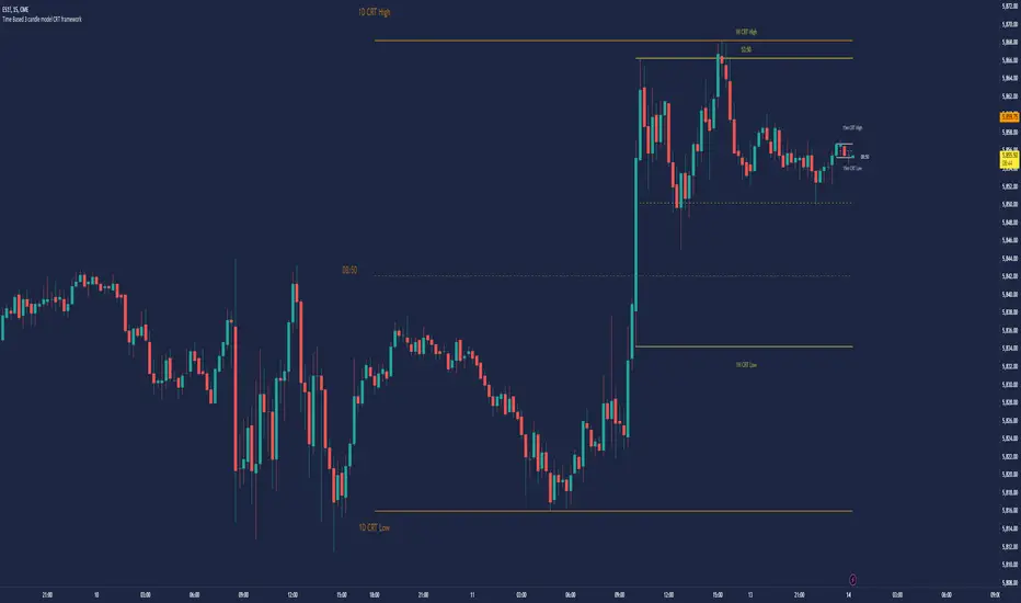
Bull/Bear Candle % Oscillator█ OVERVIEW
This script determines the proportion of bullish and bearish candles in a given sample size. It will produce an oscillator that fluctuates between 100 and -100, where values > 0 indicate more bullish candles in the sample and values < 0 indicate more bearish candles in the sample. Data produced by this oscillator is normalized around the 50% value, meaning that an even 50/50 split between bullish and bearish candles makes this oscillator produce 0; this oscillator indirectly represents the percent proportion of bullish and bearish candles in the sample (see HOW TO USE/INTERPRETATION OF DATA ).
It has two overarching settings: 'classic' and 'range'.
█ CONCEPTS
This script will cover concepts related to candlestick analysis, volumetric analysis, and lower timeframes.
Candlestick Analysis - The idea behind this script is to solely look at the candlesticks themselves and derive information from them in a given sample. It separates candles into two categories, bullish (close > open) and bearish (close < open).
If the indicator's setting is set to 'classic', the size of candles do not matter and all are assigned a value of 1 or 0.
If the indicator's setting is set to 'range', specific candle ranges modify the proportion of bullish/bearish values. Bullish candle values include all bullish candles in the set from their lows to the close, plus the lower wicks of all bearish candles. Bearish candle values include all bearish candles in the set from their highs to the close, plus the upper wicks of all bullish candles.
Volumetric Analysis - One of this script's features allows the user to modify the bullish and bearish candle proportions by its 'weight' determined by its volume compared to the sample set's total volume. Volumetric analysis for the 'range' setting are more complex than 'classic' as described below.
Lower Timeframes - For volumetric analysis to be done on candle wicks, there needed to be a way to determine how much volume had occurred in the wick by itself to find the weight of upper and lower wicks. To accomplish this, I employed PineScrypt's request.security_lower_tf function to grab OHLC values of lower timeframe candles (as well as volume) to determine how much volume had occurred in the wicks of the chart resolution's candle. The default OHLC values used here are the lows for upper wicks and highs for lower wicks. These OHLC values are then compared to the chart resolution candle's close to determine if the volume of that lower timeframe candle should be shifted to the wick weight or stay in the current weight of that candle. The reason 'low' and 'high' are used here is to guarantee that 100% of the volume of a lower timeframe candle had occurred in the wick of the candle at the current resolution (see LIMITATIONS ).
Bullish candles will exclude volume of all lower timeframe candles whose lows were greater than that candle's close. Bearish candles will exclude volume of all lower timeframe candles whose highs were less than that candle's close. These wick volumes are then divided by the volume of the sample set, and wick sizes are then multiplied by this weight before being added to their specific bullish/bearish sums (lower wicks to bullish and upper wicks to bearish).
█ FEATURES
There are 13 inputs for the user to modify the behavior/visual representation of this script.
Sample Length - This determines how many candles are in the sample set to find the proportion of bullish and bearish candles.
Colors and Invert Colors - There are three colors set by the user: a bullish color, neutral color, and bearish color. The oscillator plots two lines, one at 0 and another that represents the proportion of bullish or bearish candles in the sample set (we'll call this the 'signal line'). If the oscillator is above 0, bullish color is used, bearish otherwise. This script generates a gradient to color a filled area between the 0 line and the signal line based on the historical values of the oscillator itself and the signal line. For bullish values, the closer the signal line is to the max (or restricted max described below) that the oscillator has experienced, the more colored toward bullish color the shaded area will be, using the neutral color as a starting point. The same is applied to the bearish values using the bearish color.
There is an additional input to invert the colors so that the bearish color is associated with bullish values and vise-versa.
Calculation Type - This determines the overarching behavior of the oscillator and has two settings:
Classic - The weight of candles are either 1 if they occurred and 0 if not.
Range - The weight of candles is determined by the size of specific sections as described in CONCEPTS - Candlestick Analysis .
Volume Weighted - This enables modifying the weights of candles as described in CONCEPTS - Volumetric Analysis and Lower Timeframes based on which Calculation Type is used.
Wick Slice Resolution - This is the lower timeframe resolution that will be used to slice the chart resolution's candle when determining the volumetric weight of wicks. Lower timeframe resolutions like '1 minute' will yield more precise results as they will give more data points to go off of (see LIMITATIONS ).
Upper/Lower Wick Source - These two inputs allow the user to select which OHLC values to compare against the chart resolution's candle close when determining which lower timeframe candles will have their volumes associated with the wicks of candles being analyzed at the chart's resolution.
Restrict Min/Max Data and Restriction - This will restrict the maximum and minimum values that will be used for the signal line when comparing its value to previous oscillator values and change how the color gradient is generated for the indicator. Restriction is the number of candles back that will determine these maximum and minimum values.
Display Min/Max Guide - This will plot two lines that are colored the corresponding bullish and bearish colors which follow what the maximum and minimum values are currently for the oscillator.
█ HOW TO USE/INTERPRETATION OF DATA
As mentioned in the OVERVIEW section, this oscillator provides an indirect representation of the percent proportion of bullish or bearish candles in a given sample. If the oscillator reads 80, this does not mean that 80% of all candles in the sample were bullish . To find the percentage of candles that were bullish or bearish, the user needs to perform the following:
50% + ((|oscillator value| / 100) * 50)%
If the oscillator value is negative, the value from above will represent the percentage of bearish candles in the sample. If it is positive, this value represents the percentage of bullish candles in the sample.
Example 1 (oscillator value = 80):
50% + ((|80| / 100) * 50)%
50% + ((0.80) * 50)%
50% + 40% = 90%
90% of the candles in the sample were bullish.
Example 2 (oscillator value = -43):
50% + ((|-43| / 100) * 50)%
50% + ((0.43) * 50)%
50% + 21.5% = 71.5%
71.5% of the candles in the sample were bearish.
An example use of this indicator would be to put in a 'buy' order when its value shows a significant proportion of the sampled candles were bearish, and put in a 'sell' order when a significant proportion of candles were bullish. Potential divergences of this oscillator may also be used to plan trades accordingly such as bearish divergence - price continues higher as the oscillator decreases in value and vise-versa.*
* Nothing in this script constitutes any form of financial advice. The user is solely responsible for their trading decisions and I will not be held liable for any losses or gains incurred with the use of this script. Please proceed with caution when using this script to assist with trading decisions.
█ LIMITATIONS
Range Volumetric Weights :
Because of the conditions that must be met in order for volume to be considered part of wicks, it is possible that the default settings and their intended reasoning will not produce reliable results. If all lower timeframe candles have highs or lows that are within the body of the candle at the chart's resolution, the volume for the wicks will effectively be 0, which is not an accurate representation of those wicks. This is one of the reasons why I included the ability to change the source values used for these conditions as certain OHLC values may produce more reliable/intended results under these conditions.
Wick Slice Resolution :
PineScript restricts the number of intrabar references to 100,000 total. This script uses 3 separate request.security_lower_tf calls and has a default resolution of 1 minute. This means that if the user were to set the oscillator to the Range setting, enable volume weighted, and had the Wick Slice Resolution set to 1 minute, this script will exceed this 100,000 reference restriction within 24 days of data and will not produce any results beyond the previous 23.14 days.
Below are example uses of all the different settings of this script, these are done on the 1D chart of COINBASE:BTCUSD :
Default Settings:
Classic - Volume Weighted:
Range - no Volume Weight:
Range - Volume Weighted (1 min slices):
Range - Volume Weighted (1 hour slices):
Display Min/Max Guide - No Restriction:
Display Min/Max Guide - Restriction:
Invert Colors:
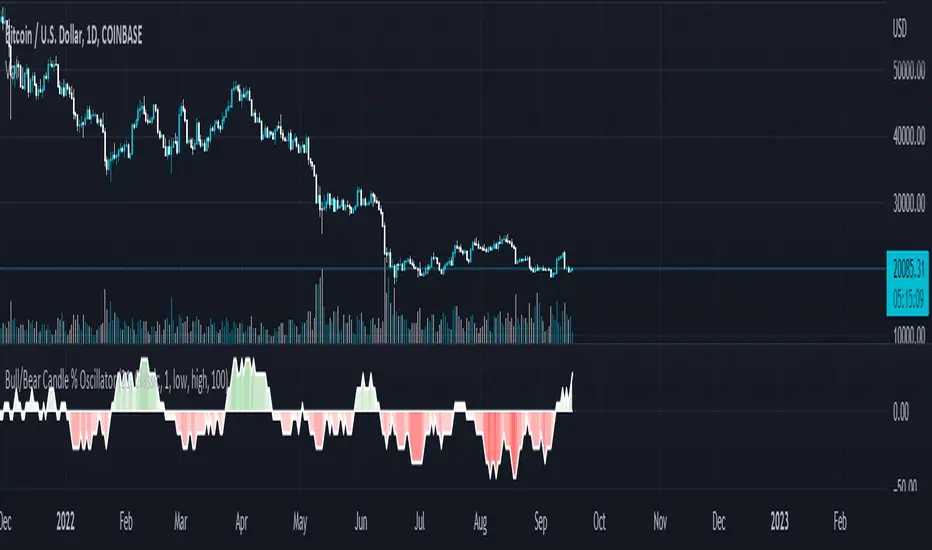
PowerX by jwitt98This strategy attempts to replicate the PowerX strategy as described in the book by by Markus Heitkoetter
Three indicators are used:
RSI (7) - An RSI above 50 indicates and uptrend. An RSI below 50 indicates a downtrend.
Slow Stochastics (14, 3, 3) - A %K above 50 indicates an uptrend. A %K below 50 indicates a downtrend.
MACD (12, 26, 9) - A MACD above the signal line indicates an uptrend. A MACD below the signal line indicates a downtrend
In addition, multiples of ADR (7) is used for setting the stops and profit targets
Setup:
When all 3 indicators are indicating an uptrend, the OHLC bar is green.
When all 3 indicators are indicating a downtrend, the OHLC bar is red.
When one or more indicators are conflicting, the OHLC bar is black
The basic rules are:
When the OHLC bar is green and the preceding bar is black or Red, enter a long stop-limit order .01 above the high of the first green bar
When the OHLC bar is red and the preceding bar is black or green, enter a short stop-limit order .01 below the low of the first red bar
If a red or black bar is encountered while in a long trade, or a green or black bar for a short trade, exit the trade at the close of that bar with a market order.
Stop losses are set by default at a multiple of 1.5 times the ADR.
Profit targets are set by default at a multiple of 3 times the ADR.
Options:
You can adjust the start and end dates for the trading range
You can configure this strategy for long only, short only, or both long and short.
You can adjust the multiples used to set the stop losses and profit targets.
There is an option to use a money management system very similar to the one described in the PowerX book. Some assumptions had to be made for cases where the equity is underwater as those cases are not clearly defined in the book. There is an option to override this behavior and keep the risk at or above the set point (2% by default), rather than further reduce the risk when equity is underwater. Position sizing is limited when using money management so as not to exceed the current strategy equity. The starting risk can be adjusted from the default of 2%.
Final notes: If you find any errors, have any questions, or have suggestions for improvements, please leave your message in the comments.
Happy trading!
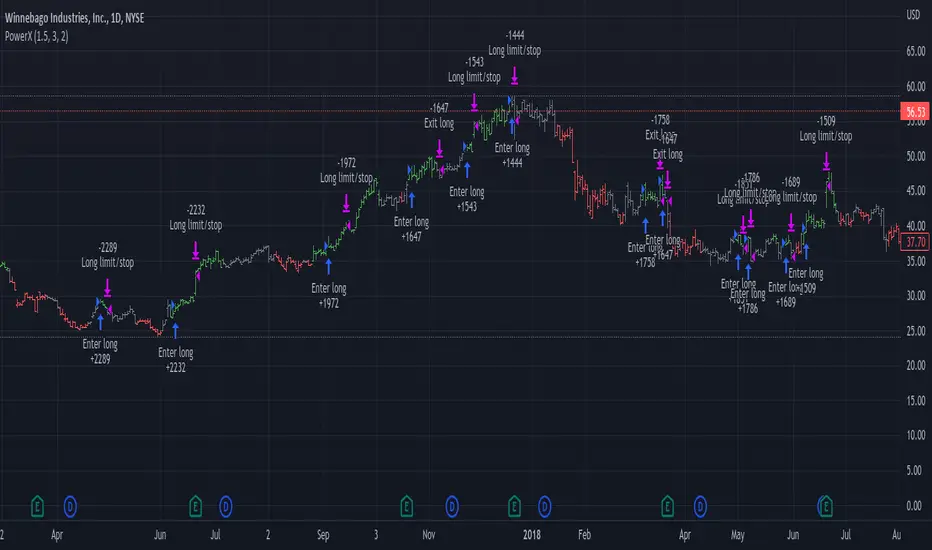
Top - Bottom Using MAThis script is used decide weather stock is overbought or oversold in given length/days from the settings.
using close difference from ohlc4 moving average ratio.
Settings Available
1) moving average length
2) Highest / Lowest ratio length
3) Difference Between Highest and Lowest Line
this script plot/display 4 lines
1) highest difference from moving averages in provided length.
2) lowest difference from moving averages in provided length.
3) ratio of moving average and ohlc4
4) linear regression moving averages of ratio of moving average and ohlc4
How to use this script
1) when ratio line is touch 2 days to highest ratio line means we are consider stock is in overbought levels or linear regression moving average above highest ratio line means overbought.
2) when ratio lines cross below its linear regression moving average then we consider final exit or book profit.
3) when linear regression moving average below lowest ratio line means stock is in oversold.
4) when linear regression moving average below lowest ratio line and linear regression line start rising after fall it means there is change in trend.
5) when linear regression moving average cross above lowest ratio line it means trend is changed and linear regression line turns green.

Fibonacci Bollinger Band ClusterThis indicator creates moving averages based on Fibonacci numbers (3-233, divided by 10 to average) sourced by high, low, and ohlc4 and plots lines based on these three. The Fib MA High line is either green or red (Fib High < Close), the Fib MA Low line is either lime or orange (Fib Low < Close), and the Fib MA OHLC4 line is constantly white. A cluster or series of Bollinger Bands is then created using the Fib MA OHLC4 line as the basis. Fibonacci-based deviations (1, 2, 3, 5, 8) are then used to create three upper and three lower Bollinger lines.
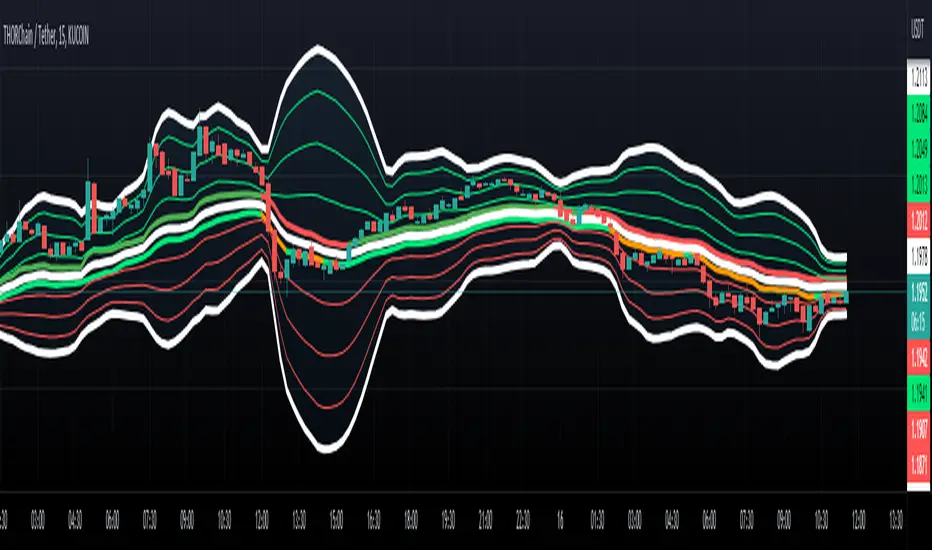
eStrategyLibrary "eStrategy"
Library contains methods which can help build custom strategy for continuous investment plans and also compare it with systematic buy and hold.
sip(startYear, initialDeposit, depositFrequency, recurringDeposit, buyPrice) Depicts systematic buy and hold over period of time
Parameters:
startYear : Year on which SIP is started
initialDeposit : Initial one time investment at the start
depositFrequency : Frequency of recurring deposit - can be monthly or weekly
recurringDeposit : Recurring deposit amount
buyPrice : Indicatinve buy price. Use high to be conservative. low, close, open, hl2, hlc3, ohlc4, hlcc4 are other options.
Returns: totalInvestment - initial + recurring deposits
totalQty - Quantity of units held for given instrument
totalEquity - Present equity
customStrategy(startYear, initialDeposit, depositFrequency, recurringDeposit, buyPrice, sellPrice, initialInvestmentPercent, recurringInvestmentPercent, signal, tradePercent) Allows users to define custom strategy and enhance systematic buy and hold by adding take profit and reloads
Parameters:
startYear : Year on which SIP is started
initialDeposit : Initial one time investment at the start
depositFrequency : Frequency of recurring deposit - can be monthly or weekly
recurringDeposit : Recurring deposit amount
buyPrice : Indicatinve buy price. Use high to be conservative. low, close, open, hl2, hlc3, ohlc4, hlcc4 are other options.
sellPrice : Indicatinve sell price. Use low to be conservative. high, close, open, hl2, hlc3, ohlc4, hlcc4 are other options.
initialInvestmentPercent : percent of amount to invest from the initial depost. Keep rest of them as cash
recurringInvestmentPercent : percent of amount to invest from recurring deposit. Keep rest of them as cash
signal : can be 1, -1 or 0. 1 means buy/reload. -1 means take profit and 0 means neither.
tradePercent : percent of amount to trade when signal is not 0. If taking profit, it will sell the percent from existing position. If reloading, it will buy with percent from cash reserve
Returns: totalInvestment - initial + recurring deposits
totalQty - Quantity of units held for given instrument
totalCash = Amount of cash held
totalEquity - Overall equity = totalQty*close + totalCash
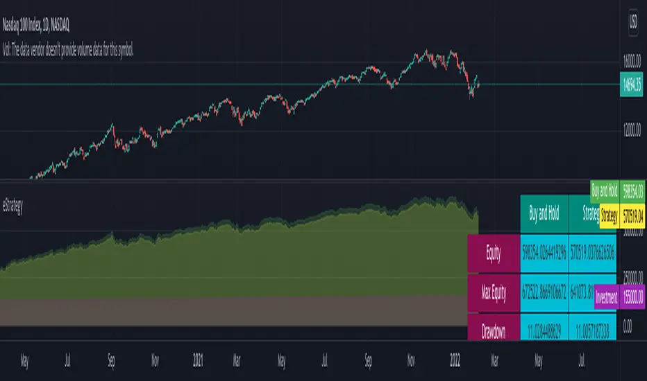
lib_Indicators_v2_DTULibrary "lib_Indicators_v2_DTU"
This library functions returns included Moving averages, indicators with factorization, functions candles, function heikinashi and more.
Created it to feed as backend of my indicator/strategy "Indicators & Combinations Framework Advanced v2 " that will be released ASAP.
This is replacement of my previous indicator (lib_indicators_DT)
I will add an indicator example which will use this indicator named as "lib_indicators_v2_DTU example" to help the usage of this library
Additionally library will be updated with more indicators in the future
NOTES:
Indicator functions returns only one series :-(
plotcandle function returns candle series
INDICATOR LIST:
hide = 'DONT DISPLAY', //Dont display & calculate the indicator. (For my framework usage)
alma = 'alma(src,len,offset=0.85,sigma=6)', //Arnaud Legoux Moving Average
ama = 'ama(src,len,fast=14,slow=100)', //Adjusted Moving Average
acdst = 'accdist()', //Accumulation/distribution index.
cma = 'cma(src,len)', //Corrective Moving average
dema = 'dema(src,len)', //Double EMA (Same as EMA with 2 factor)
ema = 'ema(src,len)', //Exponential Moving Average
gmma = 'gmma(src,len)', //Geometric Mean Moving Average
hghst = 'highest(src,len)', //Highest value for a given number of bars back.
hl2ma = 'hl2ma(src,len)', //higest lowest moving average
hma = 'hma(src,len)', //Hull Moving Average.
lgAdt = 'lagAdapt(src,len,perclen=5,fperc=50)', //Ehler's Adaptive Laguerre filter
lgAdV = 'lagAdaptV(src,len,perclen=5,fperc=50)', //Ehler's Adaptive Laguerre filter variation
lguer = 'laguerre(src,len)', //Ehler's Laguerre filter
lsrcp = 'lesrcp(src,len)', //lowest exponential esrcpanding moving line
lexp = 'lexp(src,len)', //lowest exponential expanding moving line
linrg = 'linreg(src,len,loffset=1)', //Linear regression
lowst = 'lowest(src,len)', //Lovest value for a given number of bars back.
pcnl = 'percntl(src,len)', //percentile nearest rank. Calculates percentile using method of Nearest Rank.
pcnli = 'percntli(src,len)', //percentile linear interpolation. Calculates percentile using method of linear interpolation between the two nearest ranks.
rema = 'rema(src,len)', //Range EMA (REMA)
rma = 'rma(src,len)', //Moving average used in RSI. It is the exponentially weighted moving average with alpha = 1 / length.
sma = 'sma(src,len)', //Smoothed Moving Average
smma = 'smma(src,len)', //Smoothed Moving Average
supr2 = 'super2(src,len)', //Ehler's super smoother, 2 pole
supr3 = 'super3(src,len)', //Ehler's super smoother, 3 pole
strnd = 'supertrend(src,len,period=3)', //Supertrend indicator
swma = 'swma(src,len)', //Sine-Weighted Moving Average
tema = 'tema(src,len)', //Triple EMA (Same as EMA with 3 factor)
tma = 'tma(src,len)', //Triangular Moving Average
vida = 'vida(src,len)', //Variable Index Dynamic Average
vwma = 'vwma(src,len)', //Volume Weigted Moving Average
wma = 'wma(src,len)', //Weigted Moving Average
angle = 'angle(src,len)', //angle of the series (Use its Input as another indicator output)
atr = 'atr(src,len)', //average true range. RMA of true range.
bbr = 'bbr(src,len,mult=1)', //bollinger %%
bbw = 'bbw(src,len,mult=2)', //Bollinger Bands Width. The Bollinger Band Width is the difference between the upper and the lower Bollinger Bands divided by the middle band.
cci = 'cci(src,len)', //commodity channel index
cctbb = 'cctbbo(src,len)', //CCT Bollinger Band Oscilator
chng = 'change(src,len)', //Difference between current value and previous, source - source .
cmo = 'cmo(src,len)', //Chande Momentum Oscillator. Calculates the difference between the sum of recent gains and the sum of recent losses and then divides the result by the sum of all price movement over the same period.
cog = 'cog(src,len)', //The cog (center of gravity) is an indicator based on statistics and the Fibonacci golden ratio.
cpcrv = 'copcurve(src,len)', //Coppock Curve. was originally developed by Edwin "Sedge" Coppock (Barron's Magazine, October 1962).
corrl = 'correl(src,len)', //Correlation coefficient. Describes the degree to which two series tend to deviate from their ta.sma values.
count = 'count(src,len)', //green avg - red avg
dev = 'dev(src,len)', //ta.dev() Measure of difference between the series and it's ta.sma
fall = 'falling(src,len)', //ta.falling() Test if the `source` series is now falling for `length` bars long. (Use its Input as another indicator output)
kcr = 'kcr(src,len,mult=2)', //Keltner Channels Range
kcw = 'kcw(src,len,mult=2)', //ta.kcw(). Keltner Channels Width. The Keltner Channels Width is the difference between the upper and the lower Keltner Channels divided by the middle channel.
macd = 'macd(src,len)', //macd
mfi = 'mfi(src,len)', //Money Flow Index
nvi = 'nvi()', //Negative Volume Index
obv = 'obv()', //On Balance Volume
pvi = 'pvi()', //Positive Volume Index
pvt = 'pvt()', //Price Volume Trend
rise = 'rising(src,len)', //ta.rising() Test if the `source` series is now rising for `length` bars long. (Use its Input as another indicator output)
roc = 'roc(src,len)', //Rate of Change
rsi = 'rsi(src,len)', //Relative strength Index
smosc = 'smi_osc(src,len,fast=5, slow=34)', //smi Oscillator
smsig = 'smi_sig(src,len,fast=5, slow=34)', //smi Signal
stdev = 'stdev(src,len)', //Standart deviation
trix = 'trix(src,len)' , //the rate of change of a triple exponentially smoothed moving average.
tsi = 'tsi(src,len)', //True Strength Index
vari = 'variance(src,len)', //ta.variance(). Variance is the expectation of the squared deviation of a series from its mean (ta.sma), and it informally measures how far a set of numbers are spread out from their mean.
wilpc = 'willprc(src,len)', //Williams %R
wad = 'wad()', //Williams Accumulation/Distribution.
wvad = 'wvad()' //Williams Variable Accumulation/Distribution.
}
f_func(string, float, simple, float, float, float, simple) f_func Return selected indicator value with different parameters. New version. Use extra parameters for available indicators
Parameters:
string : FuncType_ indicator from the indicator list
float : src_ close, open, high, low,hl2, hlc3, ohlc4 or any
simple : int length_ indicator length
float : p1 extra parameter-1. active on Version 2 for defining multi arguments indicator input value. ex: lagAdapt(src_, length_,LAPercLen_=p1,FPerc_=p2)
float : p2 extra parameter-2. active on Version 2 for defining multi arguments indicator input value. ex: lagAdapt(src_, length_,LAPercLen_=p1,FPerc_=p2)
float : p3 extra parameter-3. active on Version 2 for defining multi arguments indicator input value. ex: lagAdapt(src_, length_,LAPercLen_=p1,FPerc_=p2)
simple : int version_ indicator version for backward compatibility. V1:dont use extra parameters p1,p2,p3 and use default values. V2: use extra parameters for available indicators
Returns: float Return calculated indicator value
fn_heikin(float, float, float, float) fn_heikin Return given src data (open, high,low,close) as heikin ashi candle values
Parameters:
float : o_ open value
float : h_ high value
float : l_ low value
float : c_ close value
Returns: float heikin ashi open, high,low,close vlues that will be used with plotcandle
fn_plotFunction(float, string, simple, bool) fn_plotFunction Return input src data with different plotting options
Parameters:
float : src_ indicator src_data or any other series.....
string : plotingType Ploting type of the function on the screen
simple : int stochlen_ length for plotingType for stochastic and PercentRank options
bool : plotSWMA Use SWMA for smoothing Ploting
Returns: float
fn_funcPlotV2(string, float, simple, float, float, float, simple, string, simple, bool, bool) fn_funcPlotV2 Return selected indicator value with different parameters. New version. Use extra parameters fora available indicators
Parameters:
string : FuncType_ indicator from the indicator list
float : src_data_ close, open, high, low,hl2, hlc3, ohlc4 or any
simple : int length_ indicator length
float : p1 extra parameter-1. active on Version 2 for defining multi arguments indicator input value. ex: lagAdapt(src_, length_,LAPercLen_=p1,FPerc_=p2)
float : p2 extra parameter-2. active on Version 2 for defining multi arguments indicator input value. ex: lagAdapt(src_, length_,LAPercLen_=p1,FPerc_=p2)
float : p3 extra parameter-3. active on Version 2 for defining multi arguments indicator input value. ex: lagAdapt(src_, length_,LAPercLen_=p1,FPerc_=p2)
simple : int version_ indicator version for backward compatibility. V1:dont use extra parameters p1,p2,p3 and use default values. V2: use extra parameters for available indicators
string : plotingType Ploting type of the function on the screen
simple : int stochlen_ length for plotingType for stochastic and PercentRank options
bool : plotSWMA Use SWMA for smoothing Ploting
bool : log_ Use log on function entries
Returns: float Return calculated indicator value
fn_factor(string, float, simple, float, float, float, simple, simple, string, simple, bool, bool) fn_factor Return selected indicator's factorization with given arguments
Parameters:
string : FuncType_ indicator from the indicator list
float : src_data_ close, open, high, low,hl2, hlc3, ohlc4 or any
simple : int length_ indicator length
float : p1 parameter-1. active on Version 2 for defining multi arguments indicator input value. ex: lagAdapt(src_, length_,LAPercLen_=p1,FPerc_=p2)
float : p2 parameter-2. active on Version 2 for defining multi arguments indicator input value. ex: lagAdapt(src_, length_,LAPercLen_=p1,FPerc_=p2)
float : p3 parameter-3. active on Version 2 for defining multi arguments indicator input value. ex: lagAdapt(src_, length_,LAPercLen_=p1,FPerc_=p2)
simple : int version_ indicator version for backward compatibility. V1:dont use extra parameters p1,p2,p3 and use default values. V2: use extra parameters for available indicators
simple : int fact_ Add double triple, Quatr factor to selected indicator (like converting EMA to 2-DEMA, 3-TEMA, 4-QEMA...)
string : plotingType Ploting type of the function on the screen
simple : int stochlen_ length for plotingType for stochastic and PercentRank options
bool : plotSWMA Use SWMA for smoothing Ploting
bool : log_ Use log on function entries
Returns: float Return result of the function
fn_plotCandles(string, simple, float, float, float, simple, string, simple, bool, bool, bool) fn_plotCandles Return selected indicator's candle values with different parameters also heikinashi is available
Parameters:
string : FuncType_ indicator from the indicator list
simple : int length_ indicator length
float : p1 parameter-1. active on Version 2 for defining multi arguments indicator input value. ex: lagAdapt(src_, length_,LAPercLen_=p1,FPerc_=p2)
float : p2 parameter-2. active on Version 2 for defining multi arguments indicator input value. ex: lagAdapt(src_, length_,LAPercLen_=p1,FPerc_=p2)
float : p3 parameter-3. active on Version 2 for defining multi arguments indicator input value. ex: lagAdapt(src_, length_,LAPercLen_=p1,FPerc_=p2)
simple : int version_ indicator version for backward compatibility. V1:dont use extra parameters p1,p2,p3 and use default values. V2: use extra parameters for available indicators
string : plotingType Ploting type of the function on the screen
simple : int stochlen_ length for plotingType for stochastic and PercentRank options
bool : plotSWMA Use SWMA for smoothing Ploting
bool : log_ Use log on function entries
bool : plotheikin_ Use Heikin Ashi on Plot
Returns: float
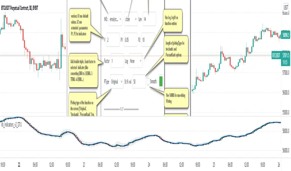
Weekday Close vs Open — Last N (per weekday)# Weekday Close vs Open - Last N Occurrences
This indicator distills every weekday's historical open-to-close behavior into a compact table so you can see how "typical" the current session is before the day even closes. It runs independently of your chart timeframe by pulling daily OHLCV data under the hood, tracking the last **N** completed occurrences for each weekday, and refreshing only when a daily bar closes. On daily charts you can also shade every past bar that matches today's weekday (excluding the in-progress session) to reinforce the pattern visually while the table remains non-repainting.
## What It Shows
- **Win/Loss/Tie counts** - how many of the last `N` occurrences closed above the open (wins), below (losses), or inside the tie threshold you define as "flat".
- **Win % heatmap** - the win column is color-coded (deep green > deep red) so you immediately recognize strong or weak weekdays.
- **Advanced metrics (optional)** - average daily volume plus the average percentage excursion above/below the open (`AvgUp%`, `AvgDn%`) for that weekday.
- **Totals row** - aggregates every weekday into one row to estimate overall hit rate and average stats across the entire data set.
- **Weekday shading (optional)** - on daily charts you can tint every bar that matches today's weekday (all Mondays, all Fridays, etc.) for instant pattern recognition.
## How It Works
1. The script requests daily OHLCV data (non-repainting) regardless of the chart timeframe.
2. When a new daily bar confirms, it packs that day's data into one of seven arrays (one per weekday). Each day contributes five floats (O/H/L/C/V) so trimming and statistics stay in lockstep.
3. A helper function (`f_dayMetrics`) scans daily history to compute average volume, average excursion above/below the open, and win/loss/tie counts for the requested weekday.
4. The table populates on the last bar of the chart session, respecting your advanced/totals toggles and keeping text at `size.normal`.
## Reading the Table
- **Win/Loss/Tie columns**: raw counts taken from your chosen `N`.
- **Win %***: excludes ties from the denominator so it reflects only decisive closes.
- **AvgUp% / AvgDn%**: typical intraday extension (high vs open, open vs low) in percent.
- **Avg Vol**: arithmetic mean of daily volume for that weekday.
- **TOTAL row**: provides a global win rate plus volume/up/down averages weighted by how many samples each weekday contributed.
## Practical Uses
- Spot weekdays that historically trend higher or lower before entering a trade.
- Compare current price action against the typical intraday range (`AvgUp%` vs today's move).
- Filter mean-reversion vs breakout setups based on the most reliable weekday patterns.
- Quickly gauge whether today is behaving "in character" by referencing the highlighted row or the optional whole-chart weekday shading.
> **Tip:** Use smaller `N` values (e.g., 10-20) for adaptive, recent behavior and larger values (50+) to capture longer-term seasonality. Tighten the tie threshold if you want almost every candle to register as win/loss, or widen it to focus only on meaningful moves.

Algorithm Predator - ML-liteAlgorithm Predator - ML-lite
This indicator combines four specialized trading agents with an adaptive multi-armed bandit selection system to identify high-probability trade setups. It is designed for swing and intraday traders who want systematic signal generation based on institutional order flow patterns , momentum exhaustion , liquidity dynamics , and statistical mean reversion .
Core Architecture
Why These Components Are Combined:
The script addresses a fundamental challenge in algorithmic trading: no single detection method works consistently across all market conditions. By deploying four independent agents and using reinforcement learning algorithms to select or blend their outputs, the system adapts to changing market regimes without manual intervention.
The Four Trading Agents
1. Spoofing Detector Agent 🎭
Detects iceberg orders through persistent volume at similar price levels over 5 bars
Identifies spoofing patterns via asymmetric wick analysis (wicks exceeding 60% of bar range with volume >1.8× average)
Monitors order clustering using simplified Hawkes process intensity tracking (exponential decay model)
Signal Logic: Contrarian—fades false breakouts caused by institutional manipulation
Best Markets: Consolidations, institutional trading windows, low-liquidity hours
2. Exhaustion Detector Agent ⚡
Calculates RSI divergence between price movement and momentum indicator over 5-bar window
Detects VWAP exhaustion (price at 2σ bands with declining volume)
Uses VPIN reversals (volume-based toxic flow dissipation) to identify momentum failure
Signal Logic: Counter-trend—enters when momentum extreme shows weakness
Best Markets: Trending markets reaching climax points, over-extended moves
3. Liquidity Void Detector Agent 💧
Measures Bollinger Band squeeze (width <60% of 50-period average)
Identifies stop hunts via 20-bar high/low penetration with immediate reversal and volume spike
Detects hidden liquidity absorption (volume >2× average with range <0.3× ATR)
Signal Logic: Breakout anticipation—enters after liquidity grab but before main move
Best Markets: Range-bound pre-breakout, volatility compression zones
4. Mean Reversion Agent 📊
Calculates price z-scores relative to 50-period SMA and standard deviation (triggers at ±2σ)
Implements Ornstein-Uhlenbeck process scoring (mean-reverting stochastic model)
Uses entropy analysis to detect algorithmic trading patterns (low entropy <0.25 = high predictability)
Signal Logic: Statistical reversion—enters when price deviates significantly from statistical equilibrium
Best Markets: Range-bound, low-volatility, algorithmically-dominated instruments
Adaptive Selection: Multi-Armed Bandit System
The script implements four reinforcement learning algorithms to dynamically select or blend agents based on performance:
Thompson Sampling (Default - Recommended):
Uses Bayesian inference with beta distributions (tracks alpha/beta parameters per agent)
Balances exploration (trying underused agents) vs. exploitation (using proven winners)
Each agent's win/loss history informs its selection probability
Lite Approximation: Uses pseudo-random sampling from price/volume noise instead of true random number generation
UCB1 (Upper Confidence Bound):
Calculates confidence intervals using: average_reward + sqrt(2 × ln(total_pulls) / agent_pulls)
Deterministic algorithm favoring agents with high uncertainty (potential upside)
More conservative than Thompson Sampling
Epsilon-Greedy:
Exploits best-performing agent (1-ε)% of the time
Explores randomly ε% of the time (default 10%, configurable 1-50%)
Simple, transparent, easily tuned via epsilon parameter
Gradient Bandit:
Uses softmax probability distribution over agent preference weights
Updates weights via gradient ascent based on rewards
Best for Blend mode where all agents contribute
Selection Modes:
Switch Mode: Uses only the selected agent's signal (clean, decisive)
Blend Mode: Combines all agents using exponentially weighted confidence scores controlled by temperature parameter (smooth, diversified)
Lock Agent Feature:
Optional manual override to force one specific agent
Useful after identifying which agent dominates your specific instrument
Only applies in Switch mode
Four choices: Spoofing Detector, Exhaustion Detector, Liquidity Void, Mean Reversion
Memory System
Dual-Layer Architecture:
Short-Term Memory: Stores last 20 trade outcomes per agent (configurable 10-50)
Long-Term Memory: Stores episode averages when short-term reaches transfer threshold (configurable 5-20 bars)
Memory Boost Mechanism: Recent performance modulates agent scores by up to ±20%
Episode Transfer: When an agent accumulates sufficient results, averages are condensed into long-term storage
Persistence: Manual restoration of learned parameters via input fields (alpha, beta, weights, microstructure thresholds)
How Memory Works:
Agent generates signal → outcome tracked after 8 bars (performance horizon)
Result stored in short-term memory (win = 1.0, loss = 0.0)
Short-term average influences agent's future scores (positive feedback loop)
After threshold met (default 10 results), episode averaged into long-term storage
Long-term patterns (weighted 30%) + short-term patterns (weighted 70%) = total memory boost
Market Microstructure Analysis
These advanced metrics quantify institutional order flow dynamics:
Order Flow Toxicity (Simplified VPIN):
Measures buy/sell volume imbalance over 20 bars: |buy_vol - sell_vol| / (buy_vol + sell_vol)
Detects informed trading activity (institutional players with non-public information)
Values >0.4 indicate "toxic flow" (informed traders active)
Lite Approximation: Uses simple open/close heuristic instead of tick-by-tick trade classification
Price Impact Analysis (Simplified Kyle's Lambda):
Measures market impact efficiency: |price_change_10| / sqrt(volume_sum_10)
Low values = large orders with minimal price impact ( stealth accumulation )
High values = retail-dominated moves with high slippage
Lite Approximation: Uses simplified denominator instead of regression-based signed order flow
Market Randomness (Entropy Analysis):
Counts unique price changes over 20 bars / 20
Measures market predictability
High entropy (>0.6) = human-driven, chaotic price action
Low entropy (<0.25) = algorithmic trading dominance (predictable patterns)
Lite Approximation: Simple ratio instead of true Shannon entropy H(X) = -Σ p(x)·log₂(p(x))
Order Clustering (Simplified Hawkes Process):
Tracks self-exciting event intensity (coordinated order activity)
Decays at 0.9× per bar, spikes +1.0 when volume >1.5× average
High intensity (>0.7) indicates clustering (potential spoofing/accumulation)
Lite Approximation: Simple exponential decay instead of full λ(t) = μ + Σ α·exp(-β(t-tᵢ)) with MLE
Signal Generation Process
Multi-Stage Validation:
Stage 1: Agent Scoring
Each agent calculates internal score based on its detection criteria
Scores must exceed agent-specific threshold (adjusted by sensitivity multiplier)
Agent outputs: Signal direction (+1/-1/0) and Confidence level (0.0-1.0)
Stage 2: Memory Boost
Agent scores multiplied by memory boost factor (0.8-1.2 based on recent performance)
Successful agents get amplified, failing agents get dampened
Stage 3: Bandit Selection/Blending
If Adaptive Mode ON:
Switch: Bandit selects single best agent, uses only its signal
Blend: All agents combined using softmax-weighted confidence scores
If Adaptive Mode OFF:
Traditional consensus voting with confidence-squared weighting
Signal fires when consensus exceeds threshold (default 70%)
Stage 4: Confirmation Filter
Raw signal must repeat for consecutive bars (default 3, configurable 2-4)
Minimum confidence threshold: 0.25 (25%) enforced regardless of mode
Trend alignment check: Long signals require trend_score ≥ -2, Short signals require trend_score ≤ 2
Stage 5: Cooldown Enforcement
Minimum bars between signals (default 10, configurable 5-15)
Prevents over-trading during choppy conditions
Stage 6: Performance Tracking
After 8 bars (performance horizon), signal outcome evaluated
Win = price moved in signal direction, Loss = price moved against
Results fed back into memory and bandit statistics
Trading Modes (Presets)
Pre-configured parameter sets:
Conservative: 85% consensus, 4 confirmations, 15-bar cooldown
Expected: 60-70% win rate, 3-8 signals/week
Best for: Swing trading, capital preservation, beginners
Balanced: 70% consensus, 3 confirmations, 10-bar cooldown
Expected: 55-65% win rate, 8-15 signals/week
Best for: Day trading, most traders, general use
Aggressive: 60% consensus, 2 confirmations, 5-bar cooldown
Expected: 50-58% win rate, 15-30 signals/week
Best for: Scalping, high-frequency trading, active management
Elite: 75% consensus, 3 confirmations, 12-bar cooldown
Expected: 58-68% win rate, 5-12 signals/week
Best for: Selective trading, high-conviction setups
Adaptive: 65% consensus, 2 confirmations, 8-bar cooldown
Expected: Varies based on learning
Best for: Experienced users leveraging bandit system
How to Use
1. Initial Setup (5 Minutes):
Select Trading Mode matching your style (start with Balanced)
Enable Adaptive Learning (recommended for automatic agent selection)
Choose Thompson Sampling algorithm (best all-around performance)
Keep Microstructure Metrics enabled for liquid instruments (>100k daily volume)
2. Agent Tuning (Optional):
Adjust Agent Sensitivity multipliers (0.5-2.0):
<0.8 = Highly selective (fewer signals, higher quality)
0.9-1.2 = Balanced (recommended starting point)
1.3 = Aggressive (more signals, lower individual quality)
Monitor dashboard for 20-30 signals to identify dominant agent
If one agent consistently outperforms, consider using Lock Agent feature
3. Bandit Configuration (Advanced):
Blend Temperature (0.1-2.0):
0.3 = Sharp decisions (best agent dominates)
0.5 = Balanced (default)
1.0+ = Smooth (equal weighting, democratic)
Memory Decay (0.8-0.99):
0.90 = Fast adaptation (volatile markets)
0.95 = Balanced (most instruments)
0.97+ = Long memory (stable trends)
4. Signal Interpretation:
Green triangle (▲): Long signal confirmed
Red triangle (▼): Short signal confirmed
Dashboard shows:
Active agent (highlighted row with ► marker)
Win rate per agent (green >60%, yellow 40-60%, red <40%)
Confidence bars (█████ = maximum confidence)
Memory size (short-term buffer count)
Colored zones display:
Entry level (current close)
Stop-loss (1.5× ATR)
Take-profit 1 (2.0× ATR)
Take-profit 2 (3.5× ATR)
5. Risk Management:
Never risk >1-2% per signal (use ATR-based stops)
Signals are entry triggers, not complete strategies
Combine with your own market context analysis
Consider fundamental catalysts and news events
Use "Confirming" status to prepare entries (not to enter early)
6. Memory Persistence (Optional):
After 50-100 trades, check Memory Export Panel
Record displayed alpha/beta/weight values for each agent
Record VPIN and Kyle threshold values
Enable "Restore From Memory" and input saved values to continue learning
Useful when switching timeframes or restarting indicator
Visual Components
On-Chart Elements:
Spectral Layers: EMA8 ± 0.5 ATR bands (dynamic support/resistance, colored by trend)
Energy Radiance: Multi-layer glow boxes at signal points (intensity scales with confidence, configurable 1-5 layers)
Probability Cones: Projected price paths with uncertainty wedges (15-bar projection, width = confidence × ATR)
Connection Lines: Links sequential signals (solid = same direction continuation, dotted = reversal)
Kill Zones: Risk/reward boxes showing entry, stop-loss, and dual take-profit targets
Signal Markers: Triangle up/down at validated entry points
Dashboard (Configurable Position & Size):
Regime Indicator: 4-level trend classification (Strong Bull/Bear, Weak Bull/Bear)
Mode Status: Shows active system (Adaptive Blend, Locked Agent, or Consensus)
Agent Performance Table: Real-time win%, confidence, and memory stats
Order Flow Metrics: Toxicity and impact indicators (when microstructure enabled)
Signal Status: Current state (Long/Short/Confirming/Waiting) with confirmation progress
Memory Panel (Configurable Position & Size):
Live Parameter Export: Alpha, beta, and weight values per agent
Adaptive Thresholds: Current VPIN sensitivity and Kyle threshold
Save Reminder: Visual indicator if parameters should be recorded
What Makes This Original
This script's originality lies in three key innovations:
1. Genuine Meta-Learning Framework:
Unlike traditional indicator mashups that simply display multiple signals, this implements authentic reinforcement learning (multi-armed bandits) to learn which detection method works best in current conditions. The Thompson Sampling implementation with beta distribution tracking (alpha for successes, beta for failures) is statistically rigorous and adapts continuously. This is not post-hoc optimization—it's real-time learning.
2. Episodic Memory Architecture with Transfer Learning:
The dual-layer memory system mimics human learning patterns:
Short-term memory captures recent performance (recency bias)
Long-term memory preserves historical patterns (experience)
Automatic transfer mechanism consolidates knowledge
Memory boost creates positive feedback loops (successful strategies become stronger)
This architecture allows the system to adapt without retraining , unlike static ML models that require batch updates.
3. Institutional Microstructure Integration:
Combines retail-focused technical analysis (RSI, Bollinger Bands, VWAP) with institutional-grade microstructure metrics (VPIN, Kyle's Lambda, Hawkes processes) typically found in academic finance literature and professional trading systems, not standard retail platforms. While simplified for Pine Script constraints, these metrics provide insight into informed vs. uninformed trading , a dimension entirely absent from traditional technical analysis.
Mashup Justification:
The four agents are combined specifically for risk diversification across failure modes:
Spoofing Detector: Prevents false breakout losses from manipulation
Exhaustion Detector: Prevents chasing extended trends into reversals
Liquidity Void: Exploits volatility compression (different regime than trending)
Mean Reversion: Provides mathematical anchoring when patterns fail
The bandit system ensures the optimal tool is automatically selected for each market situation, rather than requiring manual interpretation of conflicting signals.
Why "ML-lite"? Simplifications and Approximations
This is the "lite" version due to necessary simplifications for Pine Script execution:
1. Simplified VPIN Calculation:
Academic Implementation: True VPIN uses volume bucketing (fixed-volume bars) and tick-by-tick buy/sell classification via Lee-Ready algorithm or exchange-provided trade direction flags
This Implementation: 20-bar rolling window with simple open/close heuristic (close > open = buy volume)
Impact: May misclassify volume during ranging/choppy markets; works best in directional moves
2. Pseudo-Random Sampling:
Academic Implementation: Thompson Sampling requires true random number generation from beta distributions using inverse transform sampling or acceptance-rejection methods
This Implementation: Deterministic pseudo-randomness derived from price and volume decimal digits: (close × 100 - floor(close × 100)) + (volume % 100) / 100
Impact: Not cryptographically random; may have subtle biases in specific price ranges; provides sufficient variation for agent selection
3. Hawkes Process Approximation:
Academic Implementation: Full Hawkes process uses maximum likelihood estimation with exponential kernels: λ(t) = μ + Σ α·exp(-β(t-tᵢ)) fitted via iterative optimization
This Implementation: Simple exponential decay (0.9 multiplier) with binary event triggers (volume spike = event)
Impact: Captures self-exciting property but lacks parameter optimization; fixed decay rate may not suit all instruments
4. Kyle's Lambda Simplification:
Academic Implementation: Estimated via regression of price impact on signed order flow over multiple time intervals: Δp = λ × Δv + ε
This Implementation: Simplified ratio: price_change / sqrt(volume_sum) without proper signed order flow or regression
Impact: Provides directional indicator of impact but not true market depth measurement; no statistical confidence intervals
5. Entropy Calculation:
Academic Implementation: True Shannon entropy requires probability distribution: H(X) = -Σ p(x)·log₂(p(x)) where p(x) is probability of each price change magnitude
This Implementation: Simple ratio of unique price changes to total observations (variety measure)
Impact: Measures diversity but not true information entropy with probability weighting; less sensitive to distribution shape
6. Memory System Constraints:
Full ML Implementation: Neural networks with backpropagation, experience replay buffers (storing state-action-reward tuples), gradient descent optimization, and eligibility traces
This Implementation: Fixed-size array queues with simple averaging; no gradient-based learning, no state representation beyond raw scores
Impact: Cannot learn complex non-linear patterns; limited to linear performance tracking
7. Limited Feature Engineering:
Advanced Implementation: Dozens of engineered features, polynomial interactions (x², x³), dimensionality reduction (PCA, autoencoders), feature selection algorithms
This Implementation: Raw agent scores and basic market metrics (RSI, ATR, volume ratio); minimal transformation
Impact: May miss subtle cross-feature interactions; relies on agent-level intelligence rather than feature combinations
8. Single-Instrument Data:
Full Implementation: Multi-asset correlation analysis (sector ETFs, currency pairs, volatility indices like VIX), lead-lag relationships, risk-on/risk-off regimes
This Implementation: Only OHLCV data from displayed instrument
Impact: Cannot incorporate broader market context; vulnerable to correlated moves across assets
9. Fixed Performance Horizon:
Full Implementation: Adaptive horizon based on trade duration, volatility regime, or profit target achievement
This Implementation: Fixed 8-bar evaluation window
Impact: May evaluate too early in slow markets or too late in fast markets; one-size-fits-all approach
Performance Impact Summary:
These simplifications make the script:
✅ Faster: Executes in milliseconds vs. seconds (or minutes) for full academic implementations
✅ More Accessible: Runs on any TradingView plan without external data feeds, APIs, or compute servers
✅ More Transparent: All calculations visible in Pine Script (no black-box compiled models)
✅ Lower Resource Usage: <500 bars lookback, minimal memory footprint
⚠️ Less Precise: Approximations may reduce statistical edge by 5-15% vs. academic implementations
⚠️ Limited Scope: Cannot capture tick-level dynamics, multi-order-book interactions, or cross-asset flows
⚠️ Fixed Parameters: Some thresholds hardcoded rather than dynamically optimized
When to Upgrade to Full Implementation:
Consider professional Python/C++ versions with institutional data feeds if:
Trading with >$100K capital where precision differences materially impact returns
Operating in microsecond-competitive environments (HFT, market making)
Requiring regulatory-grade audit trails and reproducibility
Backtesting with tick-level precision for strategy validation
Need true real-time adaptation with neural network-based learning
For retail swing/day trading and position management, these approximations provide sufficient signal quality while maintaining usability, transparency, and accessibility. The core logic—multi-agent detection with adaptive selection—remains intact.
Technical Notes
All calculations use standard Pine Script built-in functions ( ta.ema, ta.atr, ta.rsi, ta.bb, ta.sma, ta.stdev, ta.vwap )
VPIN and Kyle's Lambda use simplified formulas optimized for OHLCV data (see "Lite" section above)
Thompson Sampling uses pseudo-random noise from price/volume decimal digits for beta distribution sampling
No repainting: All calculations use confirmed bar data (no forward-looking)
Maximum lookback: 500 bars (set via max_bars_back parameter)
Performance evaluation: 8-bar forward-looking window for reward calculation (clearly disclosed)
Confidence threshold: Minimum 0.25 (25%) enforced on all signals
Memory arrays: Dynamic sizing with FIFO queue management
Limitations and Disclaimers
Not Predictive: This indicator identifies patterns in historical data. It cannot predict future price movements with certainty.
Requires Human Judgment: Signals are entry triggers, not complete trading strategies. Must be confirmed with your own analysis, risk management rules, and market context.
Learning Period Required: The adaptive system requires 50-100 bars minimum to build statistically meaningful performance data for bandit algorithms.
Overfitting Risk: Restoring memory parameters from one market regime to a drastically different regime (e.g., low volatility to high volatility) may cause poor initial performance until system re-adapts.
Approximation Limitations: Simplified calculations (see "Lite" section) may underperform academic implementations by 5-15% in highly efficient markets.
No Guarantee of Profit: Past performance, whether backtested or live-traded, does not guarantee future performance. All trading involves risk of loss.
Forward-Looking Bias: Performance evaluation uses 8-bar forward window—this creates slight look-ahead for learning (though not for signals). Real-time performance may differ from indicator's internal statistics.
Single-Instrument Limitation: Does not account for correlations with related assets or broader market regime changes.
Recommended Settings
Timeframe: 15-minute to 4-hour charts (sufficient volatility for ATR-based stops; adequate bar volume for learning)
Assets: Liquid instruments with >100k daily volume (forex majors, large-cap stocks, BTC/ETH, major indices)
Not Recommended: Illiquid small-caps, penny stocks, low-volume altcoins (microstructure metrics unreliable)
Complementary Tools: Volume profile, order book depth, market breadth indicators, fundamental catalysts
Position Sizing: Risk no more than 1-2% of capital per signal using ATR-based stop-loss
Signal Filtering: Consider external confluence (support/resistance, trendlines, round numbers, session opens)
Start With: Balanced mode, Thompson Sampling, Blend mode, default agent sensitivities (1.0)
After 30+ Signals: Review agent win rates, consider increasing sensitivity of top performers or locking to dominant agent
Alert Configuration
The script includes built-in alert conditions:
Long Signal: Fires when validated long entry confirmed
Short Signal: Fires when validated short entry confirmed
Alerts fire once per bar (after confirmation requirements met)
Set alert to "Once Per Bar Close" for reliability
Taking you to school. — Dskyz, Trade with insight. Trade with anticipation.

Mystic Pulse V2.0 [CHE] Mystic Pulse V2.0 — Adaptive DI streaks with gradient intensity for clearer trend persistence
Summary
Mystic Pulse V2.0 measures directional persistence by counting how often the positive or negative directional index strengthens and dominates. These counts drive gradient colors for bars, wicks, and helper plots, so intensity reflects local momentum rather than absolute values. A windowed normalization and gamma control adapt the visuals to recent conditions, preventing one regime from overpowering the next. The result is an immediate, at-a-glance read of trend direction and stamina without relying on crossovers alone.
Motivation: Why this design?
Classical DI and ADX signals can flip during choppy phases or feel sluggish in calm regimes. This script focuses on persistence: it increments a positive or negative streak only when the corresponding directional pressure both strengthens compared with the prior bar and dominates the other side. Simple OHLC pre-smoothing reduces micro-noise, and local normalization keeps the scale relevant to the last segment of data, not a distant past.
What’s different vs. standard approaches?
Reference baseline: Traditional DI and ADX lines with crossovers and fixed-scale thresholds.
Architecture differences:
Wilder-style recursive smoothing on true range and directional movement.
Streak counters for positive and negative pressure that advance only on strengthening and dominance.
Windowed normalization and gamma shaping for visual intensity.
Wick coloring via `plotcandle` with forced overlay from a pane indicator.
Practical effect: Bars and wicks grow more vivid during sustained pressure and fade during indecision. The column plots show streak depth directly, which helps filter one-bar flips.
How it works (technical)
1. Pre-smoothing: Open, high, low, and close are averaged over a short simple moving window to dampen micro-ticks.
2. Directional inputs: True range and directional movement are formed from the smoothed prices, then recursively smoothed using a Wilder-style update that carries prior state forward.
3. DI comparison: The script derives positive and negative directional ratios relative to smoothed range. A side advances its streak when it increases compared with the previous bar and exceeds the opposite side. The other streak resets.
4. Trend score and color base: The difference between positive and negative streaks defines the active side.
5. Normalization and gamma: The absolute streak magnitude and each side’s streak are normalized within a rolling window. Gamma parameters reshape intensity so mid-range values are either compressed or emphasized.
6. Rendering:
Two column plots show positive and negative streak counts in the pane with gradient colors.
A square marker at the bottom uses the global gradient as a compact heat cue.
Bar colors on the main chart use either the gradient, neutral trend colors, or no paint depending on toggles.
Wick, border, and candle overlays are colored via `plotcandle` with forced overlay.
7. State handling: Smoothed values and counters persist across bars; initialization uses first available values without lookahead. No higher-timeframe requests are used, so repaint risk is limited to normal live-bar evolution.
Parameter Guide
Show neutral candles (fallback) — Paints main-chart bars in plain up or down colors when gradients are disabled — Default false — Use when you prefer simple up/down coloring.
Show last N shapes — Limits bottom square markers — Default 333 — Reduce if your chart gets cluttered.
ADX smoothing length — Controls the Wilder smoothing window for range and directional movement — Default 9 — Larger values increase stability but respond later.
OHLC SMA length — Pre-smoothing for inputs — Default 1 — Increase slightly on noisy assets to reduce flip risk.
Gradient barcolor — Enables gradient bar paint on the main chart — Default true — Turn off to use wicks only or neutral bars.
Wick coloring — Colors wicks, borders, and bodies via overlay — Default true — Disable if it conflicts with other overlays.
Gradient window — Lookback for local normalization — Default 100 — Shorter windows adapt faster; longer windows provide steadier intensity.
Gradient transparency — Overall transparency for gradient paints — Default 0 — Increase to make gradients subtler.
Gamma bars/shapes — Contrast for bar and shape intensity — Default 0.70 — Lower values brighten mid-tones; higher values compress them.
Gamma plots — Contrast for the column plots — Default 0.80 — Tune separately from bar intensity.
Wick transparency — Transparency for wick coloring — Default 0 — Raise to let price action show through.
Up/Down colors (dark and neon) — Base and accent colors for both directions — Defaults as provided — Adjust to match your chart theme.
Reading & Interpretation
Pane columns: The green column represents the positive streak count; the red column represents the negative streak count. Taller columns signal stronger persistence.
Gradient marker: The bottom square indicates the active side and persistence strength at a glance.
Main-chart bars and wicks: Color direction shows the dominant side; intensity reflects the normalized and gamma-shaped streak magnitude. Faded tones suggest weak or fading pressure.
Practical Workflows & Combinations
Trend following: Enter in the direction of the active side when the corresponding column expands over several bars. Confirm with structure such as higher highs and higher lows or lower highs and lower lows.
Exits and stops: Consider scaling out when intensity fades toward mid-range while structure stalls. Tighten stops after extended streaks or when wicks lose intensity.
Multi-asset/Multi-TF: Use defaults for liquid assets on intraday to swing timeframes. For highly volatile instruments, raise smoothing and the normalization window. For calm markets, lower them to regain sensitivity.
Behavior, Constraints & Performance
Repaint/confirmation: Values update during the live bar and stabilize after bar close. No historical repaint beyond normal live-bar updates.
security()/HTF: Not used; cross-timeframe repaint paths do not apply.
Resources: Declared `max_bars_back` two thousand; no explicit loops or arrays; plot and label limits are generous.
Known limits: Streak counters can remain elevated during slow reversals. Very short normalization windows can cause rapid intensity swings. Gaps or extreme spikes may temporarily distort intensity until the window adapts.
Sensible Defaults & Quick Tuning
Start with: ADX smoothing nine, OHLC SMA one, normalization window one hundred, gradient and wick coloring enabled, gamma around zero point seven to zero point eight.
Too many flips: Increase ADX smoothing and the normalization window; consider a small bump in OHLC SMA.
Too sluggish: Decrease ADX smoothing and the normalization window.
Colors overpower chart: Increase gradient and wick transparency or raise gamma to compress mid-tones.
What this indicator is—and isn’t
This is a visualization and signal layer that represents directional persistence and intensity. It does not issue trade entries or exits on its own and is not predictive. Use it alongside market structure, volume, and risk controls.
Disclaimer
The content, including any code, is for educational and informational purposes only and does not constitute financial advice or a recommendation to buy or sell any instrument. Trading involves substantial risk, including the possible loss of principal. Past performance is not indicative of future results. Always do your own research and consider consulting a qualified professional.

POC Migration Velocity (POC-MV) [PhenLabs]📊POC Migration Velocity (POC-MV)
Version: PineScript™v6
📌Description
The POC Migration Velocity indicator revolutionizes market structure analysis by tracking the movement, speed, and acceleration of Point of Control (POC) levels in real-time. This tool combines sophisticated volume distribution estimation with velocity calculations to reveal hidden market dynamics that conventional indicators miss.
POC-MV provides traders with unprecedented insight into volume-based price movement patterns, enabling the early identification of continuation and exhaustion signals before they become apparent to the broader market. By measuring how quickly and consistently the POC migrates across price levels, traders gain early warning signals for significant market shifts and can position themselves advantageously.
The indicator employs advanced algorithms to estimate intra-bar volume distribution without requiring lower timeframe data, making it accessible across all chart timeframes while maintaining sophisticated analytical capabilities.
🚀Points of Innovation
Micro-POC calculation using advanced OHLC-based volume distribution estimation
Real-time velocity and acceleration tracking normalized by ATR for cross-market consistency
Persistence scoring system that quantifies directional consistency over multiple periods
Multi-signal detection combining continuation patterns, exhaustion signals, and gap alerts
Dynamic color-coded visualization system with intensity-based feedback
Comprehensive customization options for resolution, periods, and thresholds
🔧Core Components
POC Calculation Engine: Estimates volume distribution within each bar using configurable price bands and sophisticated weighting algorithms
Velocity Measurement System: Tracks the rate of POC movement over customizable lookback periods with ATR normalization
Acceleration Calculator: Measures the rate of change of velocity to identify momentum shifts in POC migration
Persistence Analyzer: Quantifies how consistently POC moves in the same direction using exponential weighting
Signal Detection Framework: Combines trend analysis, velocity thresholds, and persistence requirements for signal generation
Visual Rendering System: Provides dynamic color-coded lines and heat ribbons based on velocity and price-POC relationships
🔥Key Features
Real-time POC calculation with 10-100 configurable price bands for optimal precision
Velocity tracking with customizable lookback periods from 5 to 50 bars
Acceleration measurement for detecting momentum changes in POC movement
Persistence scoring to validate signal strength and filter false signals
Dynamic visual feedback with blue/orange color scheme indicating bullish/bearish conditions
Comprehensive alert system for continuation patterns, exhaustion signals, and POC gaps
Adjustable information table displaying real-time metrics and current signals
Heat ribbon visualization showing price-POC relationship intensity
Multiple threshold settings for customizing signal sensitivity
Export capability for use with separate panel indicators
🎨Visualization
POC Connecting Lines: Color-coded lines showing POC levels with intensity based on velocity magnitude
Heat Ribbon: Dynamic colored ribbon around price showing POC-price basis intensity
Signal Markers: Clear exhaustion top/bottom signals with labeled shapes
Information Table: Real-time display of POC value, velocity, acceleration, basis, persistence, and current signal status
Color Gradients: Blue gradients for bullish conditions, orange gradients for bearish conditions
📖Usage Guidelines
POC Calculation Settings
POC Resolution (Price Bands): Default 20, Range 10-100. Controls the number of price bands used to estimate volume distribution within each bar
Volume Weight Factor: Default 0.7, Range 0.1-1.0. Adjusts the influence of volume in POC calculation
POC Smoothing: Default 3, Range 1-10. EMA smoothing period applied to the calculated POC to reduce noise
Velocity Settings
Velocity Lookback Period: Default 14, Range 5-50. Number of bars used to calculate POC velocity
Acceleration Period: Default 7, Range 3-20. Period for calculating POC acceleration
Velocity Significance Threshold: Default 0.5, Range 0.1-2.0. Minimum normalized velocity for continuation signals
Persistence Settings
Persistence Lookback: Default 5, Range 3-20. Number of bars examined for persistence score calculation
Persistence Threshold: Default 0.7, Range 0.5-1.0. Minimum persistence score required for continuation signals
Visual Settings
Show POC Connecting Lines: Toggle display of colored lines connecting POC levels
Show Heat Ribbon: Toggle display of colored ribbon showing POC-price relationship
Ribbon Transparency: Default 70, Range 0-100. Controls transparency level of heat ribbon
Alert Settings
Enable Continuation Alerts: Toggle alerts for continuation pattern detection
Enable Exhaustion Alerts: Toggle alerts for exhaustion pattern detection
Enable POC Gap Alerts: Toggle alerts for significant POC gaps
Gap Threshold: Default 2.0 ATR, Range 0.5-5.0. Minimum gap size to trigger alerts
✅Best Use Cases
Identifying trend continuation opportunities when POC velocity aligns with price direction
Spotting potential reversal points through exhaustion pattern detection
Confirming breakout validity by monitoring POC gap behavior
Adding volume-based context to traditional technical analysis
Managing position sizing based on POC-price basis strength
⚠️Limitations
POC calculations are estimations based on OHLC data, not true tick-by-tick volume distribution
Effectiveness may vary in low-volume or highly volatile market conditions
Requires complementary analysis tools for complete trading decisions
Signal frequency may be lower in ranging markets compared to trending conditions
Performance optimization needed for very short timeframes below 1-minute
💡What Makes This Unique
Advanced Estimation Algorithm: Sophisticated method for calculating POC without requiring lower timeframe data
Velocity-Based Analysis: Focus on POC movement dynamics rather than static levels
Comprehensive Signal Framework: Integration of continuation, exhaustion, and gap detection in one indicator
Dynamic Visual Feedback: Intensity-based color coding that adapts to market conditions
Persistence Validation: Unique scoring system to filter signals based on directional consistency
🔬How It Works
Volume Distribution Estimation:
Divides each bar into configurable price bands for volume analysis
Applies sophisticated weighting based on OHLC relationships and proximity to close
Identifies the price level with maximum estimated volume as the POC
Velocity and Acceleration Calculation:
Measures POC rate of change over specified lookback periods
Normalizes values using ATR for consistent cross-market performance
Calculates acceleration as the rate of change of velocity
Signal Generation Process:
Combines trend direction analysis using EMA crossovers
Applies velocity and persistence thresholds to filter signals
Generates continuation, exhaustion, and gap alerts based on specific criteria
💡Note:
This indicator provides estimated POC calculations based on available OHLC data and should be used in conjunction with other analysis methods. The velocity-based approach offers unique insights into market structure dynamics but requires proper risk management and complementary analysis for optimal trading decisions.
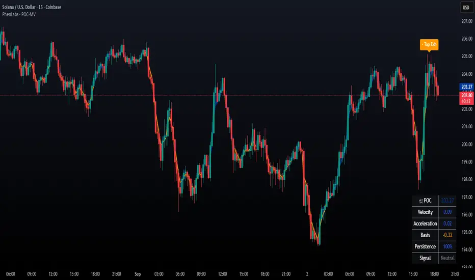
Order Blocks + Order-Flow ProxiesOrder Blocks + Order-Flow Proxies
This indicator combines structural analysis of order blocks with lightweight order-flow style proxies, providing a tool for chart annotation and contextual study. It is designed to help users visualize where significant structural shifts occur and how simple volume-based signals behave around those areas. The script does not guarantee profitable outcomes, nor does it issue financial advice. It is intended purely for research, learning, and discretionary use.
Conceptual Background
Order Blocks
An “order block” is a term often used to describe a zone on the chart where price left behind a significant reversal or imbalance before continuing strongly in the opposite direction. In practice, this can mean the last bullish or bearish candle before a strong breakout. Traders sometimes study these regions because they believe that unfilled resting orders may exist there, or simply because they mark important pivots in price structure. This indicator detects such moments by scanning for breaks of structure (BOS). When price pushes above or below recent swing levels with sufficient displacement, the script identifies the prior opposite candle as the potential order block.
Break of Structure
A break of structure in this context is defined when the closing price moves beyond the highest high or lowest low of a short lookback window. The script compares the magnitude of this break to an ATR-based displacement filter. This helps ensure that only meaningful moves are marked rather than small, random fluctuations.
Order-Flow Proxies
Traditional order flow analysis may use bid/ask data, footprint charts, or volume profiles. Because TradingView scripts cannot access true order-book data, this indicator instead uses proxy signals derived from standard chart data:
Delta (proxy): Estimated imbalance of buying vs. selling pressure, approximated using bar direction and volume.
Imbalance ratio: Normalizes delta by total volume, ranging between -1 and +1 in theory.
Cumulative Delta (CVD): Running sum of delta over time.
Effort vs. Result (EvR): A comparison between volume and actual bar movement, highlighting cases where large effort produced little result (or vice versa).
These are not real order-flow measurements, but rather simple mathematical constructs that mimic some of its logic.
How the Script Works
Detecting Break of Structure
The user specifies a swing length. When price closes above the recent high (for bullish BOS) or below the recent low (for bearish BOS), a potential shift is recorded.
To qualify, the breakout must exceed a displacement filter proportional to the ATR. This helps filter out weak moves.
Locating the Order Block Candle
Once a BOS is confirmed, the script looks back within a short window to find the last opposite-colored candle.
The high/low or open/close of that candle (depending on user settings) is marked as the potential order block zone.
Drawing and Maintaining Zones
Each order block is represented as a colored rectangle extending forward in time.
Bullish zones are teal by default, bearish zones are red.
Zones extend until invalidated (price closing or wicking beyond them, depending on user preference) or until a user-defined lifespan expires.
A pruning mechanism ensures that only the most recent set number of zones remain, preventing chart overload.
Monitoring Touches
The script checks whether the current bar’s range overlaps any existing order block.
If so, the “closest” zone is considered touched, and a label may appear on the chart.
Confirmation Filters
Touches can optionally be confirmed by order-flow proxies.
For a bullish confirmation, the following must align:
Imbalance ratio above threshold,
Delta EMA positive,
Effort vs. Result positive.
For a bearish confirmation, the opposite holds true.
Optionally, a higher-timeframe EMA slope filter can gate these confirmations. For example, a bullish confirmation may only be accepted if the higher-timeframe EMA is sloping upward.
Alerts
Users may create alerts based on conditions such as “bullish touch confirmed” or “bearish touch confirmed.”
Alerts can be gated to only fire after bar close, reducing intrabar noise.
Standard alertcondition calls are provided, and optional inline alert() calls can be enabled.
Inputs and Customization
Structure & OB
Swing length: Defines how many bars back to check for BOS.
ATR length & displacement factor: Adjust sensitivity for structural breaks.
Body vs. wick reference: Choose whether zones are based on candle bodies or full ranges.
Invalidation rule: Pick between wick breach or close beyond the level.
Lifespan (bars): Limit how long a zone remains active.
Max keep: Cap the number of zones stored to reduce clutter.
Order-Flow Proxies
Delta mode: Choose between “Close vs Previous Close” or “Body” for delta calculation.
EMA length: Smooths the delta/imbalance series.
Z-score lookback: Defines the averaging window for EvR.
Confirmation thresholds: Adjust the imbalance levels required for long/short confirmation.
Higher Timeframe Filter
Enable HTF gate: Optional filter requiring higher-timeframe EMA slope alignment.
HTF timeframe & EMA length: Configurable for context alignment.
Style
Colors and transparency for bullish and bearish zones.
Border color customization.
Alerts
Enable inline alerts: Optional direct calls to alert().
Alerts on bar close only: Helps avoid multiple firings during bar formation.
Practical Use
This tool is best seen as a way to annotate charts and to study how simple volume-derived signals behave near important structural levels. Some users may:
Observe whether order blocks line up with later price reactions.
Study how imbalance or cumulative delta conditions align with these zones.
Use it in a discretionary workflow to highlight areas of interest for deeper analysis.
Because the proxies are based only on candle OHLCV data, they are approximations. They cannot replace true depth-of-market analysis. Similarly, order block detection here is one specific algorithmic interpretation; other traders may define order blocks differently.
Limitations and Disclaimers
This indicator does not predict future price movement.
It does not access real order book or tick-by-tick data. All signals are derived from bar OHLCV.
Past performance of signals or zones does not guarantee future results.
The script is for educational and informational purposes only. It is not financial advice.
Users should test thoroughly, adjust parameters to their own instruments and timeframes, and use it in combination with broader analysis.
Summary
The Order Blocks + Order-Flow Proxies script is an experimental study tool that:
Detects potential order blocks using a displacement-filtered break of structure.
Marks these zones as boxes that persist until invalidation or expiry.
Provides lightweight order-flow-style proxies such as delta, imbalance, CVD, and effort vs. result.
Allows confirmation of zone touches through these proxies and optional higher-timeframe context.
Offers flexible customization, alerting, and chart-style options.
It is not a trading system by itself but rather a framework for studying price/volume behavior around structurally significant areas. With careful exploration, it can give users new ways to visualize market structure and to understand how simple flow-like measures behave in those contexts.

RSI Candlestick Oscillator [LuxAlgo]The RSI Candlestick Oscillator displays a traditional Relative Strength Index (RSI) as candlesticks. This indicator references OHLC data to locate each candlestick point relative to the current RSI Value, leading to a more accurate representation of the Open, High, Low, and Close price of each candlestick in the context of RSI.
In addition to the candlestick display, Divergences are detected from the RSI candlestick highs and lows and can be displayed over price on the chart.
🔶 USAGE
Translating candlesticks into the RSI oscillator is not a new concept and has been attempted many times before. This indicator stands out because of the specific method used to determine the candlestick OHLC values. When compared to other RSI Candlestick indicators, you will find that this indicator clearly and definitively correlates better to the on-chart price action.
Traditionally, the RSI indicator is simply one running value based on (typically) the close price of the chart. By introducing high, low, and open values into the oscillator, we can better gauge the specific price action throughout the intrabar movements.
Interactions with the RSI levels can now take multiple forms, whether it be a full-bodied breakthrough or simply a wick test. Both can provide a new analysis of price action alongside RSI.
An example of wick interactions and full-bodied interactions can be seen below.
As a result of the candlestick display, divergences become simpler to spot. Since the candlesticks on the RSI closely resemble the candlesticks on the chart, when looking for divergence between the chart and RSI, it is more obvious when the RSI and price are diverging.
The divergences in this indicator not only show on the RSI oscillator, but also overlay on the price chart for clearer understanding.
🔹 Filtering Divergence
With the candlesticks generating high and low RSI values, we can better sense divergences from price, since these points are generally going to be more dramatic than the (close) RSI value.
This indicator displays each type of divergence:
Bullish Divergence
Bearish Divergence
Hidden Bullish Divergence
Hidden Bearish Divergence
From these, we get many less-than-useful indications, since every single divergence from price is not necessarily of great importance.
The Divergence Filter disregards any divergence detected that does not extend outside the RSI upper or lower values.
This does not replace good judgment, but this filter can be helpful in focusing attention towards the extremes of RSI for potential reversal spotting from divergence.
🔶 DETAILS
In order to get the desired results for a display that resembles price action while following RSI, we must scale. The scaling is the most important part of this indicator.
To summarize the process:
Identify a range on Price and RSI
Consider them as equal to create a scaling factor
Use the scaling factor to locate RSI's "Price equivalent" Upper, Lower, & Mid on the Chart
Use those prices (specifically the RSI Mid) to check how far each OHLC value lies from it
Use those differences to translate the price back to the RSI Oscillator, pinning the OHLC values at their relative location to our anchor (RSI Mid)
🔹 RSI Channel
To better understand, and for your convenience, the indicator includes the option to display the RSI Channel on the chart. This channel helps to visualize where the scaled RSI values are relative to price.
If you analyze the RSI channel, you are likely to notice that the price movement throughout the channel matches the same movement witnessed in the RSI Oscillator below. This makes sense since they are the exact same thing displayed on different scales.
🔹 Scaling the Open
While the scaling method used is important, and provides a very close view of the real price bar's relative locations on the RSI oscillator… It is designed for a single purpose.
The scaling does NOT make the price candles display perfectly on the RSI oscillator.
The largest place where this is noticeable is with the opening of each candle.
For this reason, we have included a setting that modifies the opening of each RSI candle to be more accurate to the chart's price candles.
This setting positions the current bar's opening RSI candlestick value accurately relative to the price's open location to the previous closing price. As seen below.
🔶 SETTINGS
🔹 RSI Candles
RSI Length: Sets the Length for the RSI Oscillator.
Overbought/Oversold Levels: Sets the Overbought and Oversold levels for the RSI Oscillator.
Scale Open for Chart Accuracy: As described above, scales the open of each candlestick bar to more accurately portray the chart candlesticks.
🔹 Divergence
Show on Chart: Choose to display divergence line on the chart as well as on the Oscillator.
Divergence Length: Sets the pivot width for divergence detection. Normal Fractal Pivot Detection is used.
Divergence Style: Change color and line style for Regular and Hidden divergences, as well as toggle their display.
Divergence Filter: As described above, toggle on or off divergence filtering.
🔹 RSI Channel
Toggle: Display RSI Channel on Chart.
Color: Change RSI Channel Color
