VaR Market Sentiment by TenozenHello there! I am excited to share with you my new trading concept implemented in the "VaR Market Sentiment" indicator. But before that, let me explain what VaR is. VaR, or Value at Risk, is an indicator that helps you identify the worst-case scenario of a market movement based on a percentile/confidence level. This means that it calculates the worst moves, whether it's a buy or sell, based on the timeframe you're using.
Now, let's discuss how VaR Market Sentiment works. It uses a historical VaR to calculate the worst move either if the market goes up or down based on a percentile/confidence level. The default setting is the 95th percentile, which means that the market is unlikely to hit your SL level within the day if you're using a daily timeframe, etc.
To determine the strength of a candle, it subtracts the value of both sides based on the returns of the current timeframe with the VaR value (Bullish VaR - Bullish Returns, Bearish VaR - Bearish Returns). If the result is above the mean, the current candle is potentially weak. Conversely, if the result is below the mean, the current candle is potentially strong. The deviation shows critical sentiments, where if the market is above the deviation, it means that the current candle is really weak. If it's below the deviation, it means that the current candle is really strong.
It's important to note that this indicator needs other supporting indicators such as trend-following or mean reversion indicators based on your trading style. Also, as a follow-up to my previous concept, I called out that the market has what's called "power." And for now, I conclude that VaR Market Sentiment is the "power."
I'm going to share more helpful indicators in the future! I hope this indicator will be helpful for you guys! Ciao!
Поиск скриптов по запросу "VAR+计量模型+黄金期货"

Explaining VARExplaining VAR
Best to use on a Monthly Timeframe with a Ticker that exists longer then 2 years (example Bitcoin )
Then open the console so you can read and follow the instructions and explanation in the script
-> Perhaps technically some things could be better explained, but the main goal here is to explain 'var' in a rather simple way
Hope this helps, cheers!

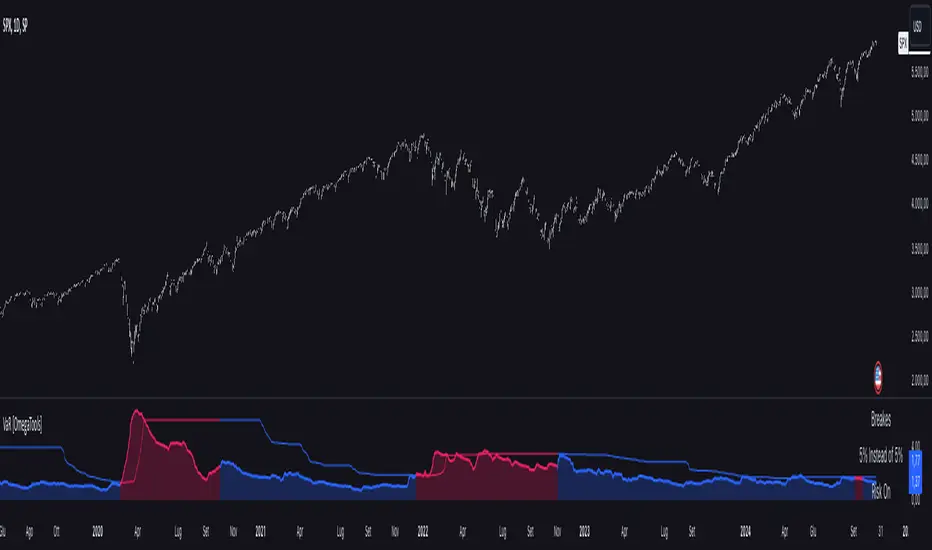
Value at Risk [OmegaTools]The "Value at Risk" (VaR) indicator is a powerful financial risk management tool that helps traders estimate the potential losses in a portfolio over a specified period of time, given a certain level of confidence. VaR is widely used by financial institutions, traders, and risk managers to assess the probability of portfolio losses in both normal and volatile market conditions. This TradingView script implements a comprehensive VaR calculation using several models, allowing users to visualize different risk scenarios and adjust their trading strategies accordingly.
Concept of Value at Risk
Value at Risk (VaR) is a statistical technique used to measure the likelihood of losses in a portfolio or financial asset due to market risks. In essence, it answers the question: "What is the maximum potential loss that could occur in a given portfolio over a specific time horizon, with a certain confidence level?" For instance, if a portfolio has a one-day 95% VaR of $10,000, it means that there is a 95% chance the portfolio will not lose more than $10,000 in a single day. Conversely, there is a 5% chance of losing more than $10,000. VaR is a key risk management tool for portfolio managers and traders because it quantifies potential losses in monetary terms, allowing for better-informed decision-making.
There are several ways to calculate VaR, and this indicator script incorporates three of the most commonly used models:
Historical VaR: This approach uses historical returns to estimate potential losses. It is based purely on past price data, assuming that the past distribution of returns is indicative of future risks.
Variance-Covariance VaR: This model assumes that asset returns follow a normal distribution and that the risk can be summarized using the mean and standard deviation of past returns. It is a parametric method that is widely used in financial risk management.
Exponentially Weighted Moving Average (EWMA) VaR: In this model, recent data points are given more weight than older data. This dynamic approach allows the VaR estimation to react more quickly to changes in market volatility, which is particularly useful during periods of market stress. This model uses the Exponential Weighted Moving Average Volatility Model.
How the Script Works
The script starts by offering users a set of customizable input settings. The first input allows the user to choose between two main calculation modes: "All" or "OCT" (Only Current Timeframe). In the "All" mode, the script calculates VaR using all available methodologies—Historical, Variance-Covariance, and EWMA—providing a comprehensive risk overview. The "OCT" mode narrows the calculation to the current timeframe, which can be particularly useful for intraday traders who need a more focused view of risk.
The next input is the lookback window, which defines the number of historical periods used to calculate VaR. Commonly used lookback periods include 21 days (approximately one month), 63 days (about three months), and 252 days (roughly one year), with the script supporting up to 504 days for more extended historical analysis. A longer lookback period provides a more comprehensive picture of risk but may be less responsive to recent market conditions.
The confidence level is another important setting in the script. This represents the probability that the loss will not exceed the VaR estimate. Standard confidence levels are 90%, 95%, and 99%. A higher confidence level results in a more conservative risk estimate, meaning that the calculated VaR will reflect a more extreme loss scenario.
In addition to these core settings, the script allows users to customize the visual appearance of the indicator. For example, traders can choose different colors for "Bullish" (Risk On), "Bearish" (Risk Off), and "Neutral" phases, as well as colors for highlighting "Breaks" in the data, where returns exceed the calculated VaR. These visual cues make it easy to identify periods of heightened risk at a glance.
The actual VaR calculation is broken down into several models, starting with the Historical VaR calculation. This is done by computing the logarithmic returns of the asset's closing prices and then using linear interpolation to determine the percentile corresponding to the desired confidence level. This percentile represents the potential loss in the asset over the lookback period.
Next, the script calculates Variance-Covariance VaR using the mean and standard deviation of the historical returns. The standard deviation is multiplied by a z-score corresponding to the chosen confidence level (e.g., 1.645 for 95% confidence), and the resulting value is subtracted from the mean return to arrive at the VaR estimate.
The EWMA VaR model uses the EWMA for the sigma parameter, the standard deviation, obtaining a specific dynamic in the volatility. It is particularly useful in volatile markets where recent price behavior is more indicative of future risk than older data.
For traders interested in intraday risk management, the script provides several methods to adjust VaR calculations for lower timeframes. By using intraday returns and scaling them according to the chosen timeframe, the script provides a dynamic view of risk throughout the trading day. This is especially important for short-term traders who need to manage their exposure during high-volatility periods within the same day. The script also incorporates an EWMA model for intraday data, which gives greater weight to the most recent intraday price movements.
In addition to calculating VaR, the script also attempts to detect periods where the asset's returns exceed the estimated VaR threshold, referred to as "Breaks." When the returns breach the VaR limit, the script highlights these instances on the chart, allowing traders to quickly identify periods of extreme risk. The script also calculates the average of these breaks and displays it for comparison, helping traders understand how frequently these high-risk periods occur.
The script further visualizes the risk scenario using a risk phase classification system. Depending on the level of risk, the script categorizes the market as either "Risk On," "Risk Off," or "Risk Neutral." In "Risk On" mode, the market is considered bullish, and the indicator displays a green background. In "Risk Off" mode, the market is bearish, and the background turns red. If the market is neither strongly bullish nor bearish, the background turns neutral, signaling a balanced risk environment.
Traders can customize whether they want to see this risk phase background, along with toggling the display of the various VaR models, the intraday methods, and the break signals. This flexibility allows traders to tailor the indicator to their specific needs, whether they are day traders looking for quick intraday insights or longer-term investors focused on historical risk analysis.
The "Risk On" and "Risk Off" phases calculated by this Value at Risk (VaR) script introduce a novel approach to market risk assessment, offering traders an advanced toolset to gauge market sentiment and potential risk levels dynamically. These risk phases are built on a combination of traditional VaR methodologies and proprietary logic to create a more responsive and intuitive way to manage exposure in both normal and volatile market conditions. This method of classifying market conditions into "Risk On," "Risk Off," or "Risk Neutral" is not something that has been traditionally associated with VaR, making it a groundbreaking addition to this indicator.
How the "Risk On" and "Risk Off" Phases Are Calculated
In typical VaR implementations, the focus is on calculating the potential losses at a given confidence level without providing an overall market outlook. This script, however, introduces a unique risk classification system that takes the output of various VaR models and translates it into actionable signals for traders, marking whether the market is in a Risk On, Risk Off, or Risk Neutral phase.
The Risk On and Risk Off phases are primarily determined by comparing the current returns of the asset to the average VaR calculated across several different methods, including Historical VaR, Variance-Covariance VaR, and EWMA VaR. Here's how the process works:
1. Threshold Setting and Effect Calculation: The script first computes the average VaR using the selected models. It then checks whether the current returns (expressed as a negative value to signify loss) exceed the average VaR value. If the current returns surpass the calculated VaR threshold, this indicates that the actual market risk is higher than expected, signaling a potential shift in market conditions.
2. Break Analysis: In addition to monitoring whether returns exceed the average VaR, the script counts the number of instances within the lookback period where this breach occurs. This is referred to as the "break effect." For each period in the lookback window, the script checks whether the returns surpass the calculated VaR threshold and increments a counter. The percentage of periods where this breach occurs is then calculated as the "effect" or break percentage.
3. Dual Effect Check (if "Double" Risk Scenario is selected): When the user chooses the "Double" risk scenario mode, the script performs two layers of analysis. First, it calculates the effect of returns exceeding the VaR threshold for the current timeframe. Then, it calculates the effect for the lower intraday timeframe as well. Both effects are compared to the user-defined confidence level (e.g., 95%). If both effects exceed the confidence level, the market is deemed to be in a high-risk situation, thus triggering a Risk Off phase. If both effects fall below the confidence level, the market is classified as Risk On.
4. Risk Phases Determination: The final risk phase is determined by analyzing these effects in relation to the confidence level:
- Risk On: If the calculated effect of breaks is lower than the confidence level (e.g., fewer than 5% of periods show returns exceeding the VaR threshold for a 95% confidence level), the market is considered to be in a relatively safe state, and the script signals a "Risk On" phase. This is indicative of bullish conditions where the potential for extreme loss is minimal.
- Risk Off: If the break effect exceeds the confidence level (e.g., more than 5% of periods show returns breaching the VaR threshold), the market is deemed to be in a high-risk state, and the script signals a "Risk Off" phase. This indicates bearish market conditions where the likelihood of significant losses is higher.
- Risk Neutral: If the break effect hovers near the confidence level or if there is no clear trend indicating a shift toward either extreme, the market is classified as "Risk Neutral." In this phase, neither bulls nor bears are dominant, and traders should remain cautious.
The phase color that the script uses helps visualize these risk phases. The background will turn green in Risk On conditions, red in Risk Off conditions, and gray in Risk Neutral phases, providing immediate visual feedback on market risk. In addition to this, when the "Double" risk scenario is selected, the background will only turn green or red if both the current and intraday timeframes confirm the respective risk phase. This double-checking process ensures that traders are only given a strong signal when both longer-term and short-term risks align, reducing the likelihood of false signals.
A New Way of Using Value at Risk
This innovative Risk On/Risk Off classification, based on the interaction between VaR thresholds and market returns, represents a significant departure from the traditional use of Value at Risk as a pure risk measurement tool. Typically, VaR is employed as a backward-looking measure of risk, providing a static estimate of potential losses over a given timeframe with no immediate actionable feedback on current market conditions. This script, however, dynamically interprets VaR results to create a forward-looking, real-time signal that informs traders whether they are operating in a favorable (Risk On) or unfavorable (Risk Off) environment.
By incorporating the "break effect" analysis and allowing users to view the VaR breaches as a percentage of past occurrences, the script adds a predictive element that can be used to time market entries and exits more effectively. This **dual-layer risk analysis**, particularly when using the "Double" scenario mode, adds further granularity by considering both current timeframe and intraday risks. Traders can therefore make more informed decisions not just based on historical risk data, but on how the market is behaving in real-time relative to those risk benchmarks.
This approach transforms the VaR indicator from a risk monitoring tool into a decision-making system that helps identify favorable trading opportunities while alerting users to potential market downturns. It provides a more holistic view of market conditions by combining both statistical risk measurement and intuitive phase-based market analysis. This level of integration between VaR methodologies and real-time signal generation has not been widely seen in the world of trading indicators, marking this script as a cutting-edge tool for risk management and market sentiment analysis.
I would like to express my sincere gratitude to @skewedzeta for his invaluable contribution to the final script. From generating fresh ideas to applying his expertise in reviewing the formula, his support has been instrumental in refining the outcome.
Value at Risk (VaR/CVaR) - Stop Loss ToolThis script calculates Value at Risk (VaR) and Conditional Value at Risk (CVaR) over a configurable T-bar forward horizon, based on historical T-bar log returns. It plots projected price thresholds that reflect the worst X% of historical return outcomes, helping set statistically grounded stop-loss levels.
A 95% 5-day VaR of −3% means: “In the worst 5% of all historical 5-day periods, losses were 3% or more.” If you're bullish, and your thesis is correct, price should not behave like one of those worst-case scenarios. So if the market starts trading below that 5-day VaR level, it may indicate that your long bias is invalidated, and a stop-loss near that level can help protect against further downside consistent with tail-risk behavior.
How it's different:
Unlike ATR or standard deviation-based methods, which measure recent volatility magnitude, VaR/CVaR incorporate both the magnitude and **likelihood** (5% chance for example) of adverse moves. This makes it better suited for risk-aware position sizing and exits grounded in actual historical return distributions.
How to use for stop placement:
- Set your holding horizon (T) and confidence level (e.g., 95%) in the inputs.
- The script plots a price level below which only the worst 5% (or chosen %) of T-bar returns have historically occurred (VaR).
- If price approaches or breaches the VaR line, your bullish/bearish thesis may be invalidated.
- CVaR gives a deeper threshold: the average loss **if** things go worse than VaR — useful for a secondary or emergency stop.
FURTHER NOTES FROM SOURCE CODE:
//======================================================================//
// If you're bullish (expecting the price to go up), then under normal circumstances, prices should not behave like they do on the worst-case days.
// If they are — you're probably wrong, or something unexpected is happening. Basically, returns shouldn't be exhibiting downside tail-like behavior if you're bullish.
// VaR(95%, T) gives the threshold below which the price falls only 5% of the time historically, over T days/bars and considering N historical samples.
// CVaR tells you the expected/average price level if that adverse move continues
// Caveats:
// For a variety of reasons, VaR underestimates volatility, despite using historical returns directly rather than making normality assumptions
// as is the case with the standard historicalvol/bollinger band/stdev/ATR approaches)
// Volatility begets volatility (volatility clustering), and VaR is not a conditional probability on recent volatility so it likely underestimates the true volatility of an adverse event
// Regieme shifts occur (bullish phase after prolonged bearish behavior), so upside/short VaR would underestimate the best-case days in the beginning of that move, depending on lookahead horizon/sampling period
// News/events happen, and maybe your sampling period doesn't contain enough event-driven returns to form reliable stats
// In general of course, this tool assumes past return distributions are reflective of forward risk (not the case in non-stationary time series)
// Thus, this tool is not predictive — it shows historical tail risk, not guaranteed outcomes.
// Also, when forming log-returns, overlapping windows of returns are used (to get more samples), but this introduces autocorrelation (if it wasn't there already). This means again, the true VaR is underestimated.
// Description:
// This script calculates and plots both Value at Risk (VaR) and
// Conditional Value at Risk (CVaR) for a given confidence level, using
// historical log returns. It computes both long-side (left tail) and
// short-side (right tail) risk, and converts them into price thresholds (red and green lines respectively).
//
// Key Concepts:
// - VaR: "There is a 95% chance the loss will be less than this value over T days. Represents the 95th-percentile worst empirical returns observed in the sampling period, over T bars.
// - CVaR: "Given that the loss exceeds the VaR, the average of those worst 5% losses is this value. (blue line)" Expected tail loss. If the worst case breached, how bad can it get on average
// - For shorts, the script computes the mirror (right-tail) equivalents.
// - Use T-day log returns if estimating risk over multiple days forward.
// - You can see instances where the VaR for time T, was surpassed historically with the "backtest" boolean
//
// Usage for Stop-Loss:
// - LONG POSITIONS:
// • 95th percentile means, 5% of the time (1 in 20 times) you'd expect to get a VaR level loss (touch the red line), over the next T bars.
// • VaR threshold = minimum price expected with (1 – confidence)% chance.
// • CVaR threshold = expected price if that worst-case zone is breached.
// → Use as potential stop-loss (VaR) or disaster stop (CVaR). If you're bullish (and you're right), price should not be exhibiting returns consistent with the worst 5% of days/T_bars historically.
//======================================================================//

IU VaR (Value at Risk) Historical MethodThis Pine Script indicator calculates the **Value at Risk (VaR)** using the **Historical Method** to help traders understand potential losses during a given period( Chart Timeframe) with a specific level of confidence.
What is Value at Risk (VaR) ?
Value at Risk (VaR) is a measure used in finance to estimate the potential loss in value of an asset, portfolio, or investment over a specific time period, given normal market conditions, and at a certain confidence level.
Example:
Suppose you invest ₹1,00,000 in stocks. A VaR of 5% at a 95% confidence level means:
- There is a **95% chance** that you won’t lose more than **₹5,000** in a day.
- Conversely, there is a **5% chance** that your loss could exceed ₹5,000 in a day.
VaR is a helpful tool for understanding risk and making informed investment decisions!
How It Works:
1. The indicator calculates the percentage difference between consecutive bars.
2. The differences are sorted, and the VaR is determined based on the assurance level you specify.
3. A label displays the VaR value on the chart, indicating the potential maximum loss with the selected assurance level within one period eg - ( 1h, 4h , 1D, 1W, 1M etc as per your chart timeframe )
Key Features:
- Customizable Assurance Level:
Set the confidence level (e.g., 95%) to determine the probability of loss.
-Historical Approach:
Uses the past percentage changes in price to calculate the risk.
-Clear Insights:
Displays the calculated VaR value on the chart with an informative tooltip explaining the risk.
Use this tool to better understand your market exposure and manage risk!

Value At Risk Channel [AstrideUnicorn]The Value at Risk Channel (VaR Channel) is a trading indicator designed to help traders control the level of risk exposure in their positions. The user can select a time period and a probability value, and the indicator will plot the upper and lower limits that the price can reach during the selected time period with the given probability.
CONCEPTS
The indicator is based on the Value at Risk (VaR) calculation. VaR is an important metric in risk management that quantifies the degree of potential financial loss within a position, portfolio or company over a specific period of time. It is widely used by financial institutions like banks and investment companies to forecast the extent and likelihood of potential losses in their portfolios.
We use the so-called “historical method” to compute VaR. The algorithm looks at the history of past returns and creates a histogram that represents the statistical distribution of past returns. Assuming that the returns follow a normal distribution, one can assign a probability to each value of return. The probability of a specific return value is determined by the distribution percentile to which it belongs.
HOW TO USE
Let’s assume you want to plot the upper and lower limits that price will reach within 4 hours with 5% probability. To do this, go to the indicator Settings tab and set the Timeframe parameter to "4 hours'' and the Probability parameter to 5.0.
You can use the indicator to set your Stop-Loss at the price level where it will trigger with low probability. And what's more, you can measure and control the probability of triggering.
You can also see how likely it is that the price will reach your Take-Profit within a specific period of time. For example, you expect your target level to be reached within a week. To determine this probability, set the Timeframe parameter to "1 week" and adjust the Probability parameter so that the upper or lower limit of your VaR channel is close to your Take-Profit level. The resulting Probability parameter value will show the probability of reaching your target in the expected time.
The indicator can be a useful tool for measuring and managing risk, as well as for developing and fine-tuning trading strategies. If you find other uses for the indicator, feel free to share them in the comments!
SETTINGS
Timeframe - sets the time period, during which the price can reach the upper or lower bound of the VaR channel with the probability, set by the Probability parameter.
Probability - specifies the probability with which the price can reach the upper or lower bound of the VaR channel during the time period specified by the Timeframe parameter.
Window - specifies the length of history (number of historical bars) used for VaR calculation.

"Swap" - Bool/Position/Value : Array / Matrix / Var AutoswapLibrary "swap"
Side / Boundary Based All Types Swapper
- three automagical types for Arrays, Matrixes, and Variables
-- no signal : Long/ Short position autoswap
-- true / false : Boolean based side choice
-- Src / Thresh : if source is above or below the threshold
- two operating modes for variables, Holding mode only for arrays/matrixes
-- with two items, will automatically change between the two caveat is it does not delete table/box/line(fill VAR items automatically)
-- with three items, a neutral is available for NA input or neutral
- one function name for all of them. One import name that's easy to type/remember
-- make life easy for your conditional items.
side(source, thresh, _a, _b, _c)
side Change outputs based on position or a crossing level
Parameters:
source : (float) OPTIONAL value input
thresh : (float) OPTIONAL boundary line to cross
_a : (any) if Long/True/Above
_b : (any) if Short/False/Below
_c : (any) OPTIONAL NOT FOR MTX OR ARR... Neutral Item, if var/varip on a/b it will leave behind, ie, a table or box or line will not erase , if it's a varip you're sending in.
Returns: first, second, or third items based on input conditions
Please notify if bugs found.
Thanks.

Education: INDEXThis is an INDEX page where educational links/scripts are sorted in the script itself (see below)
For example:
- where is the link of the 'var' article/idea?
-> search in the script comments below for Keywords -> var -> look for the date ->
now you will find the link at the date of update

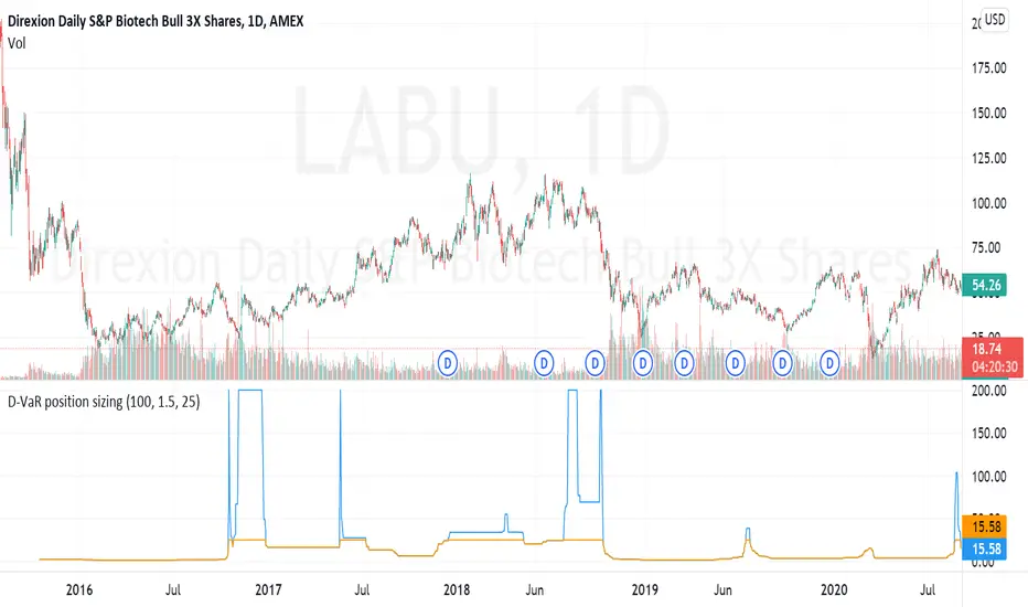
D-VaR position sizingThe D-VaR position sizing method was created by David Varadi. It's based on the concept of Value at Risk (VaR) - a widely used measure of the risk of loss in a portfolio based on the statistical analysis of historical price trends and volatilities. You can set the Percent Risk between 1 (lower) and 1.5 (higher); as well as, cap the % of Equity used in the position. The indicator plots the % of equity recommended based on the parameters you set.
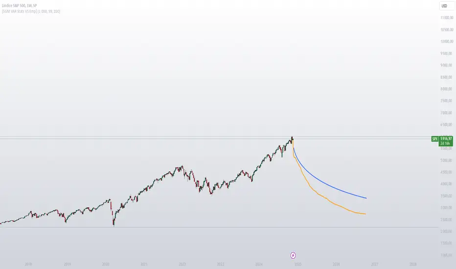
[SGM VaR Stats VS Empirical]Main Functions
Logarithmic Returns & Historical Data
Calculates logarithmic returns from closing prices.
Stores these returns in a dynamic array with a configurable maximum size.
Approximation of the Inverse Error Function
Uses an approximation of the erfinv function to calculate z-scores for given confidence levels.
Basic Statistics
Mean: Calculates the average of the data in the array.
Standard Deviation: Measures the dispersion of returns.
Median: Provides a more robust measure of central tendency for skewed distributions.
Z-Score: Converts a confidence level into a standard deviation multiplier.
Empirical vs. Statistical Projection
Empirical Projection
Based on the median of cumulative returns for each projected period.
Applies an adjustable confidence filter to exclude extreme values.
Statistical Projection
Relies on the mean and standard deviation of historical returns.
Incorporates a standard deviation multiplier for confidence-adjusted projections.
PolyLines (Graphs)
Generates projections visually through polylines:
Statistical Polyline (Blue): Based on traditional statistical methods.
Empirical Polyline (Orange): Derived from empirical data analysis.
Projection Customization
Maximum Data Size: Configurable limit for the historical data array (max_array_size).
Confidence Level: Adjustable by the user (conf_lvl), affects the width of the confidence bands.
Projection Length: Configurable number of projected periods (length_projection).
Key Steps
Capture logarithmic returns and update the historical data array.
Calculate basic statistics (mean, median, standard deviation).
Perform projections:
Empirical: Based on the median of cumulative returns.
Statistical: Based on the mean and standard deviation.
Visualization:
Compare statistical and empirical projections using polylines.
Utility
This script allows users to compare:
Traditional Statistical Projections: Based on mathematical properties of historical returns.
Empirical Projections: Relying on direct historical observations.
Divergence or convergence of these lines also highlights the presence of skewness or kurtosis in the return distribution.
Ideal for traders and financial analysts looking to assess an asset’s potential future performance using combined statistical and empirical approaches.
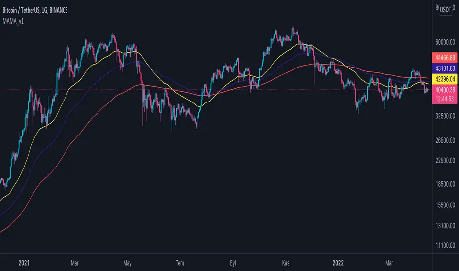
Multi Adjustable Moving Averages(MAMA) with Auto FibonacciMulti Adjustable Moving Averages(MAMA) with Auto Fibonacci
There are 10 moving averages in this indicator. There are 8 different types of moving averages to choose from.
You can also easily set the desired periods, colors and line thicknesses for each moving average from the first page.
It contains Auto Fibonacci as it is used a lot with moving averages. Those who want can easily add from the interface.
Below are the types of moving averages included;
SMA : Simple Moving Average
EMA : Exponential Moving Average
WMA : Weighted Moving Average
TMA : Triangular Moving Average
VAR : Variable Index Dynamic Moving Average a.k.a. VIDYA
WWMA : Welles Wilder's Moving Average
ZLEMA : Zero Lag Exponential Moving Average
TSF : True Strength Force
Alert ;
You can set an alarm on the cross(over or under) of the moving averages you want.
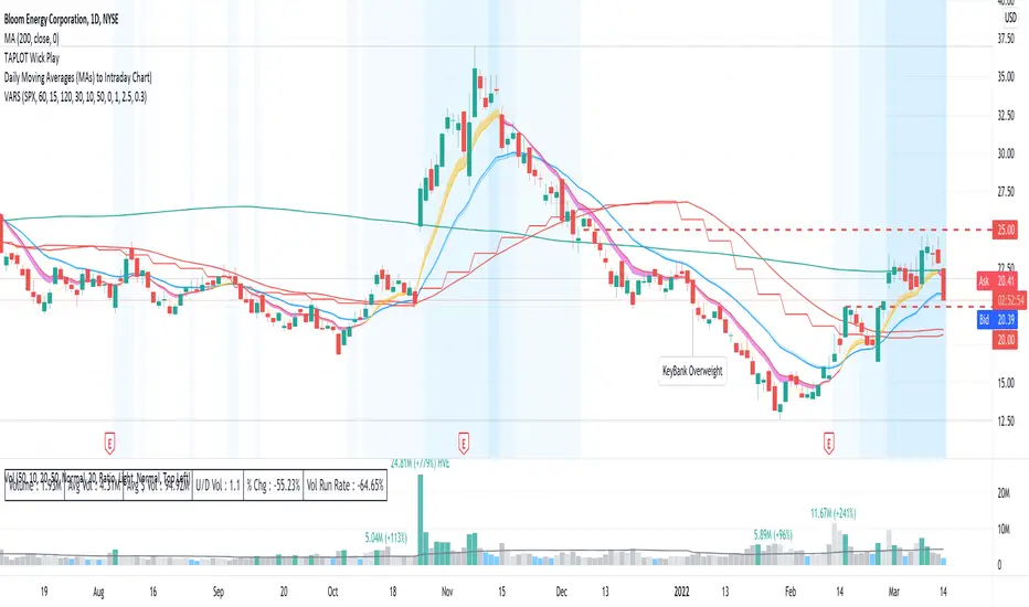
Volatility Adapted Relative StrengthVARS uses a stock's ALPHA in comparison to the SPX to determine whether there is RS on an volatility adjusted basis.
Universal Ratio Trend Matrix [InvestorUnknown]The Universal Ratio Trend Matrix is designed for trend analysis on asset/asset ratios, supporting up to 40 different assets. Its primary purpose is to help identify which assets are outperforming others within a selection, providing a broad overview of market trends through a matrix of ratios. The indicator automatically expands the matrix based on the number of assets chosen, simplifying the process of comparing multiple assets in terms of performance.
Key features include the ability to choose from a narrow selection of indicators to perform the ratio trend analysis, allowing users to apply well-defined metrics to their comparison.
Drawback: Due to the computational intensity involved in calculating ratios across many assets, the indicator has a limitation related to loading speed. TradingView has time limits for calculations, and for users on the basic (free) plan, this could result in frequent errors due to exceeded time limits. To use the indicator effectively, users with any paid plans should run it on timeframes higher than 8h (the lowest timeframe on which it managed to load with 40 assets), as lower timeframes may not reliably load.
Indicators:
RSI_raw: Simple function to calculate the Relative Strength Index (RSI) of a source (asset price).
RSI_sma: Calculates RSI followed by a Simple Moving Average (SMA).
RSI_ema: Calculates RSI followed by an Exponential Moving Average (EMA).
CCI: Calculates the Commodity Channel Index (CCI).
Fisher: Implements the Fisher Transform to normalize prices.
Utility Functions:
f_remove_exchange_name: Strips the exchange name from asset tickers (e.g., "INDEX:BTCUSD" to "BTCUSD").
f_remove_exchange_name(simple string name) =>
string parts = str.split(name, ":")
string result = array.size(parts) > 1 ? array.get(parts, 1) : name
result
f_get_price: Retrieves the closing price of a given asset ticker using request.security().
f_constant_src: Checks if the source data is constant by comparing multiple consecutive values.
Inputs:
General settings allow users to select the number of tickers for analysis (used_assets) and choose the trend indicator (RSI, CCI, Fisher, etc.).
Table settings customize how trend scores are displayed in terms of text size, header visibility, highlighting options, and top-performing asset identification.
The script includes inputs for up to 40 assets, allowing the user to select various cryptocurrencies (e.g., BTCUSD, ETHUSD, SOLUSD) or other assets for trend analysis.
Price Arrays:
Price values for each asset are stored in variables (price_a1 to price_a40) initialized as na. These prices are updated only for the number of assets specified by the user (used_assets).
Trend scores for each asset are stored in separate arrays
// declare price variables as "na"
var float price_a1 = na, var float price_a2 = na, var float price_a3 = na, var float price_a4 = na, var float price_a5 = na
var float price_a6 = na, var float price_a7 = na, var float price_a8 = na, var float price_a9 = na, var float price_a10 = na
var float price_a11 = na, var float price_a12 = na, var float price_a13 = na, var float price_a14 = na, var float price_a15 = na
var float price_a16 = na, var float price_a17 = na, var float price_a18 = na, var float price_a19 = na, var float price_a20 = na
var float price_a21 = na, var float price_a22 = na, var float price_a23 = na, var float price_a24 = na, var float price_a25 = na
var float price_a26 = na, var float price_a27 = na, var float price_a28 = na, var float price_a29 = na, var float price_a30 = na
var float price_a31 = na, var float price_a32 = na, var float price_a33 = na, var float price_a34 = na, var float price_a35 = na
var float price_a36 = na, var float price_a37 = na, var float price_a38 = na, var float price_a39 = na, var float price_a40 = na
// create "empty" arrays to store trend scores
var a1_array = array.new_int(40, 0), var a2_array = array.new_int(40, 0), var a3_array = array.new_int(40, 0), var a4_array = array.new_int(40, 0)
var a5_array = array.new_int(40, 0), var a6_array = array.new_int(40, 0), var a7_array = array.new_int(40, 0), var a8_array = array.new_int(40, 0)
var a9_array = array.new_int(40, 0), var a10_array = array.new_int(40, 0), var a11_array = array.new_int(40, 0), var a12_array = array.new_int(40, 0)
var a13_array = array.new_int(40, 0), var a14_array = array.new_int(40, 0), var a15_array = array.new_int(40, 0), var a16_array = array.new_int(40, 0)
var a17_array = array.new_int(40, 0), var a18_array = array.new_int(40, 0), var a19_array = array.new_int(40, 0), var a20_array = array.new_int(40, 0)
var a21_array = array.new_int(40, 0), var a22_array = array.new_int(40, 0), var a23_array = array.new_int(40, 0), var a24_array = array.new_int(40, 0)
var a25_array = array.new_int(40, 0), var a26_array = array.new_int(40, 0), var a27_array = array.new_int(40, 0), var a28_array = array.new_int(40, 0)
var a29_array = array.new_int(40, 0), var a30_array = array.new_int(40, 0), var a31_array = array.new_int(40, 0), var a32_array = array.new_int(40, 0)
var a33_array = array.new_int(40, 0), var a34_array = array.new_int(40, 0), var a35_array = array.new_int(40, 0), var a36_array = array.new_int(40, 0)
var a37_array = array.new_int(40, 0), var a38_array = array.new_int(40, 0), var a39_array = array.new_int(40, 0), var a40_array = array.new_int(40, 0)
f_get_price(simple string ticker) =>
request.security(ticker, "", close)
// Prices for each USED asset
f_get_asset_price(asset_number, ticker) =>
if (used_assets >= asset_number)
f_get_price(ticker)
else
na
// overwrite empty variables with the prices if "used_assets" is greater or equal to the asset number
if barstate.isconfirmed // use barstate.isconfirmed to avoid "na prices" and calculation errors that result in empty cells in the table
price_a1 := f_get_asset_price(1, asset1), price_a2 := f_get_asset_price(2, asset2), price_a3 := f_get_asset_price(3, asset3), price_a4 := f_get_asset_price(4, asset4)
price_a5 := f_get_asset_price(5, asset5), price_a6 := f_get_asset_price(6, asset6), price_a7 := f_get_asset_price(7, asset7), price_a8 := f_get_asset_price(8, asset8)
price_a9 := f_get_asset_price(9, asset9), price_a10 := f_get_asset_price(10, asset10), price_a11 := f_get_asset_price(11, asset11), price_a12 := f_get_asset_price(12, asset12)
price_a13 := f_get_asset_price(13, asset13), price_a14 := f_get_asset_price(14, asset14), price_a15 := f_get_asset_price(15, asset15), price_a16 := f_get_asset_price(16, asset16)
price_a17 := f_get_asset_price(17, asset17), price_a18 := f_get_asset_price(18, asset18), price_a19 := f_get_asset_price(19, asset19), price_a20 := f_get_asset_price(20, asset20)
price_a21 := f_get_asset_price(21, asset21), price_a22 := f_get_asset_price(22, asset22), price_a23 := f_get_asset_price(23, asset23), price_a24 := f_get_asset_price(24, asset24)
price_a25 := f_get_asset_price(25, asset25), price_a26 := f_get_asset_price(26, asset26), price_a27 := f_get_asset_price(27, asset27), price_a28 := f_get_asset_price(28, asset28)
price_a29 := f_get_asset_price(29, asset29), price_a30 := f_get_asset_price(30, asset30), price_a31 := f_get_asset_price(31, asset31), price_a32 := f_get_asset_price(32, asset32)
price_a33 := f_get_asset_price(33, asset33), price_a34 := f_get_asset_price(34, asset34), price_a35 := f_get_asset_price(35, asset35), price_a36 := f_get_asset_price(36, asset36)
price_a37 := f_get_asset_price(37, asset37), price_a38 := f_get_asset_price(38, asset38), price_a39 := f_get_asset_price(39, asset39), price_a40 := f_get_asset_price(40, asset40)
Universal Indicator Calculation (f_calc_score):
This function allows switching between different trend indicators (RSI, CCI, Fisher) for flexibility.
It uses a switch-case structure to calculate the indicator score, where a positive trend is denoted by 1 and a negative trend by 0. Each indicator has its own logic to determine whether the asset is trending up or down.
// use switch to allow "universality" in indicator selection
f_calc_score(source, trend_indicator, int_1, int_2) =>
int score = na
if (not f_constant_src(source)) and source > 0.0 // Skip if you are using the same assets for ratio (for example BTC/BTC)
x = switch trend_indicator
"RSI (Raw)" => RSI_raw(source, int_1)
"RSI (SMA)" => RSI_sma(source, int_1, int_2)
"RSI (EMA)" => RSI_ema(source, int_1, int_2)
"CCI" => CCI(source, int_1)
"Fisher" => Fisher(source, int_1)
y = switch trend_indicator
"RSI (Raw)" => x > 50 ? 1 : 0
"RSI (SMA)" => x > 50 ? 1 : 0
"RSI (EMA)" => x > 50 ? 1 : 0
"CCI" => x > 0 ? 1 : 0
"Fisher" => x > x ? 1 : 0
score := y
else
score := 0
score
Array Setting Function (f_array_set):
This function populates an array with scores calculated for each asset based on a base price (p_base) divided by the prices of the individual assets.
It processes multiple assets (up to 40), calling the f_calc_score function for each.
// function to set values into the arrays
f_array_set(a_array, p_base) =>
array.set(a_array, 0, f_calc_score(p_base / price_a1, trend_indicator, int_1, int_2))
array.set(a_array, 1, f_calc_score(p_base / price_a2, trend_indicator, int_1, int_2))
array.set(a_array, 2, f_calc_score(p_base / price_a3, trend_indicator, int_1, int_2))
array.set(a_array, 3, f_calc_score(p_base / price_a4, trend_indicator, int_1, int_2))
array.set(a_array, 4, f_calc_score(p_base / price_a5, trend_indicator, int_1, int_2))
array.set(a_array, 5, f_calc_score(p_base / price_a6, trend_indicator, int_1, int_2))
array.set(a_array, 6, f_calc_score(p_base / price_a7, trend_indicator, int_1, int_2))
array.set(a_array, 7, f_calc_score(p_base / price_a8, trend_indicator, int_1, int_2))
array.set(a_array, 8, f_calc_score(p_base / price_a9, trend_indicator, int_1, int_2))
array.set(a_array, 9, f_calc_score(p_base / price_a10, trend_indicator, int_1, int_2))
array.set(a_array, 10, f_calc_score(p_base / price_a11, trend_indicator, int_1, int_2))
array.set(a_array, 11, f_calc_score(p_base / price_a12, trend_indicator, int_1, int_2))
array.set(a_array, 12, f_calc_score(p_base / price_a13, trend_indicator, int_1, int_2))
array.set(a_array, 13, f_calc_score(p_base / price_a14, trend_indicator, int_1, int_2))
array.set(a_array, 14, f_calc_score(p_base / price_a15, trend_indicator, int_1, int_2))
array.set(a_array, 15, f_calc_score(p_base / price_a16, trend_indicator, int_1, int_2))
array.set(a_array, 16, f_calc_score(p_base / price_a17, trend_indicator, int_1, int_2))
array.set(a_array, 17, f_calc_score(p_base / price_a18, trend_indicator, int_1, int_2))
array.set(a_array, 18, f_calc_score(p_base / price_a19, trend_indicator, int_1, int_2))
array.set(a_array, 19, f_calc_score(p_base / price_a20, trend_indicator, int_1, int_2))
array.set(a_array, 20, f_calc_score(p_base / price_a21, trend_indicator, int_1, int_2))
array.set(a_array, 21, f_calc_score(p_base / price_a22, trend_indicator, int_1, int_2))
array.set(a_array, 22, f_calc_score(p_base / price_a23, trend_indicator, int_1, int_2))
array.set(a_array, 23, f_calc_score(p_base / price_a24, trend_indicator, int_1, int_2))
array.set(a_array, 24, f_calc_score(p_base / price_a25, trend_indicator, int_1, int_2))
array.set(a_array, 25, f_calc_score(p_base / price_a26, trend_indicator, int_1, int_2))
array.set(a_array, 26, f_calc_score(p_base / price_a27, trend_indicator, int_1, int_2))
array.set(a_array, 27, f_calc_score(p_base / price_a28, trend_indicator, int_1, int_2))
array.set(a_array, 28, f_calc_score(p_base / price_a29, trend_indicator, int_1, int_2))
array.set(a_array, 29, f_calc_score(p_base / price_a30, trend_indicator, int_1, int_2))
array.set(a_array, 30, f_calc_score(p_base / price_a31, trend_indicator, int_1, int_2))
array.set(a_array, 31, f_calc_score(p_base / price_a32, trend_indicator, int_1, int_2))
array.set(a_array, 32, f_calc_score(p_base / price_a33, trend_indicator, int_1, int_2))
array.set(a_array, 33, f_calc_score(p_base / price_a34, trend_indicator, int_1, int_2))
array.set(a_array, 34, f_calc_score(p_base / price_a35, trend_indicator, int_1, int_2))
array.set(a_array, 35, f_calc_score(p_base / price_a36, trend_indicator, int_1, int_2))
array.set(a_array, 36, f_calc_score(p_base / price_a37, trend_indicator, int_1, int_2))
array.set(a_array, 37, f_calc_score(p_base / price_a38, trend_indicator, int_1, int_2))
array.set(a_array, 38, f_calc_score(p_base / price_a39, trend_indicator, int_1, int_2))
array.set(a_array, 39, f_calc_score(p_base / price_a40, trend_indicator, int_1, int_2))
a_array
Conditional Array Setting (f_arrayset):
This function checks if the number of used assets is greater than or equal to a specified number before populating the arrays.
// only set values into arrays for USED assets
f_arrayset(asset_number, a_array, p_base) =>
if (used_assets >= asset_number)
f_array_set(a_array, p_base)
else
na
Main Logic
The main logic initializes arrays to store scores for each asset. Each array corresponds to one asset's performance score.
Setting Trend Values: The code calls f_arrayset for each asset, populating the respective arrays with calculated scores based on the asset prices.
Combining Arrays: A combined_array is created to hold all the scores from individual asset arrays. This array facilitates further analysis, allowing for an overview of the performance scores of all assets at once.
// create a combined array (work-around since pinescript doesn't support having array of arrays)
var combined_array = array.new_int(40 * 40, 0)
if barstate.islast
for i = 0 to 39
array.set(combined_array, i, array.get(a1_array, i))
array.set(combined_array, i + (40 * 1), array.get(a2_array, i))
array.set(combined_array, i + (40 * 2), array.get(a3_array, i))
array.set(combined_array, i + (40 * 3), array.get(a4_array, i))
array.set(combined_array, i + (40 * 4), array.get(a5_array, i))
array.set(combined_array, i + (40 * 5), array.get(a6_array, i))
array.set(combined_array, i + (40 * 6), array.get(a7_array, i))
array.set(combined_array, i + (40 * 7), array.get(a8_array, i))
array.set(combined_array, i + (40 * 8), array.get(a9_array, i))
array.set(combined_array, i + (40 * 9), array.get(a10_array, i))
array.set(combined_array, i + (40 * 10), array.get(a11_array, i))
array.set(combined_array, i + (40 * 11), array.get(a12_array, i))
array.set(combined_array, i + (40 * 12), array.get(a13_array, i))
array.set(combined_array, i + (40 * 13), array.get(a14_array, i))
array.set(combined_array, i + (40 * 14), array.get(a15_array, i))
array.set(combined_array, i + (40 * 15), array.get(a16_array, i))
array.set(combined_array, i + (40 * 16), array.get(a17_array, i))
array.set(combined_array, i + (40 * 17), array.get(a18_array, i))
array.set(combined_array, i + (40 * 18), array.get(a19_array, i))
array.set(combined_array, i + (40 * 19), array.get(a20_array, i))
array.set(combined_array, i + (40 * 20), array.get(a21_array, i))
array.set(combined_array, i + (40 * 21), array.get(a22_array, i))
array.set(combined_array, i + (40 * 22), array.get(a23_array, i))
array.set(combined_array, i + (40 * 23), array.get(a24_array, i))
array.set(combined_array, i + (40 * 24), array.get(a25_array, i))
array.set(combined_array, i + (40 * 25), array.get(a26_array, i))
array.set(combined_array, i + (40 * 26), array.get(a27_array, i))
array.set(combined_array, i + (40 * 27), array.get(a28_array, i))
array.set(combined_array, i + (40 * 28), array.get(a29_array, i))
array.set(combined_array, i + (40 * 29), array.get(a30_array, i))
array.set(combined_array, i + (40 * 30), array.get(a31_array, i))
array.set(combined_array, i + (40 * 31), array.get(a32_array, i))
array.set(combined_array, i + (40 * 32), array.get(a33_array, i))
array.set(combined_array, i + (40 * 33), array.get(a34_array, i))
array.set(combined_array, i + (40 * 34), array.get(a35_array, i))
array.set(combined_array, i + (40 * 35), array.get(a36_array, i))
array.set(combined_array, i + (40 * 36), array.get(a37_array, i))
array.set(combined_array, i + (40 * 37), array.get(a38_array, i))
array.set(combined_array, i + (40 * 38), array.get(a39_array, i))
array.set(combined_array, i + (40 * 39), array.get(a40_array, i))
Calculating Sums: A separate array_sums is created to store the total score for each asset by summing the values of their respective score arrays. This allows for easy comparison of overall performance.
Ranking Assets: The final part of the code ranks the assets based on their total scores stored in array_sums. It assigns a rank to each asset, where the asset with the highest score receives the highest rank.
// create array for asset RANK based on array.sum
var ranks = array.new_int(used_assets, 0)
// for loop that calculates the rank of each asset
if barstate.islast
for i = 0 to (used_assets - 1)
int rank = 1
for x = 0 to (used_assets - 1)
if i != x
if array.get(array_sums, i) < array.get(array_sums, x)
rank := rank + 1
array.set(ranks, i, rank)
Dynamic Table Creation
Initialization: The table is initialized with a base structure that includes headers for asset names, scores, and ranks. The headers are set to remain constant, ensuring clarity for users as they interpret the displayed data.
Data Population: As scores are calculated for each asset, the corresponding values are dynamically inserted into the table. This is achieved through a loop that iterates over the scores and ranks stored in the combined_array and array_sums, respectively.
Automatic Extending Mechanism
Variable Asset Count: The code checks the number of assets defined by the user. Instead of hardcoding the number of rows in the table, it uses a variable to determine the extent of the data that needs to be displayed. This allows the table to expand or contract based on the number of assets being analyzed.
Dynamic Row Generation: Within the loop that populates the table, the code appends new rows for each asset based on the current asset count. The structure of each row includes the asset name, its score, and its rank, ensuring that the table remains consistent regardless of how many assets are involved.
// Automatically extending table based on the number of used assets
var table table = table.new(position.bottom_center, 50, 50, color.new(color.black, 100), color.white, 3, color.white, 1)
if barstate.islast
if not hide_head
table.cell(table, 0, 0, "Universal Ratio Trend Matrix", text_color = color.white, bgcolor = #010c3b, text_size = fontSize)
table.merge_cells(table, 0, 0, used_assets + 3, 0)
if not hide_inps
table.cell(table, 0, 1,
text = "Inputs: You are using " + str.tostring(trend_indicator) + ", which takes: " + str.tostring(f_get_input(trend_indicator)),
text_color = color.white, text_size = fontSize), table.merge_cells(table, 0, 1, used_assets + 3, 1)
table.cell(table, 0, 2, "Assets", text_color = color.white, text_size = fontSize, bgcolor = #010c3b)
for x = 0 to (used_assets - 1)
table.cell(table, x + 1, 2, text = str.tostring(array.get(assets, x)), text_color = color.white, bgcolor = #010c3b, text_size = fontSize)
table.cell(table, 0, x + 3, text = str.tostring(array.get(assets, x)), text_color = color.white, bgcolor = f_asset_col(array.get(ranks, x)), text_size = fontSize)
for r = 0 to (used_assets - 1)
for c = 0 to (used_assets - 1)
table.cell(table, c + 1, r + 3, text = str.tostring(array.get(combined_array, c + (r * 40))),
text_color = hl_type == "Text" ? f_get_col(array.get(combined_array, c + (r * 40))) : color.white, text_size = fontSize,
bgcolor = hl_type == "Background" ? f_get_col(array.get(combined_array, c + (r * 40))) : na)
for x = 0 to (used_assets - 1)
table.cell(table, x + 1, x + 3, "", bgcolor = #010c3b)
table.cell(table, used_assets + 1, 2, "", bgcolor = #010c3b)
for x = 0 to (used_assets - 1)
table.cell(table, used_assets + 1, x + 3, "==>", text_color = color.white)
table.cell(table, used_assets + 2, 2, "SUM", text_color = color.white, text_size = fontSize, bgcolor = #010c3b)
table.cell(table, used_assets + 3, 2, "RANK", text_color = color.white, text_size = fontSize, bgcolor = #010c3b)
for x = 0 to (used_assets - 1)
table.cell(table, used_assets + 2, x + 3,
text = str.tostring(array.get(array_sums, x)),
text_color = color.white, text_size = fontSize,
bgcolor = f_highlight_sum(array.get(array_sums, x), array.get(ranks, x)))
table.cell(table, used_assets + 3, x + 3,
text = str.tostring(array.get(ranks, x)),
text_color = color.white, text_size = fontSize,
bgcolor = f_highlight_rank(array.get(ranks, x)))

Correlation HeatMap Matrix Data [TradingFinder]🔵 Introduction
Correlation is a statistical measure that shows the degree and direction of a linear relationship between two assets.
Its value ranges from -1 to +1 : +1 means perfect positive correlation, 0 means no linear relationship, and -1 means perfect negative correlation.
In financial markets, correlation is used for portfolio diversification, risk management, pairs trading, intermarket analysis, and identifying divergences.
Correlation HeatMap Matrix Data TradingFinder is a Pine Script v6 library that calculates and returns raw correlation matrix data between up to 20 symbols. It only provides the data – it does not draw or render the heatmap – making it ideal for use in other scripts that handle visualization or further analysis. The library uses ta.correlation for fast and accurate calculations.
It also includes two helper functions for visual styling :
CorrelationColor(corr) : takes the correlation value as input and generates a smooth gradient color, ranging from strong negative to strong positive correlation.
CorrelationTextColor(corr) : takes the correlation value as input and returns a text color that ensures optimal contrast over the background color.
Library
"Correlation_HeatMap_Matrix_Data_TradingFinder"
CorrelationColor(corr)
Parameters:
corr (float)
CorrelationTextColor(corr)
Parameters:
corr (float)
Data_Matrix(Corr_Period, Sym_1, Sym_2, Sym_3, Sym_4, Sym_5, Sym_6, Sym_7, Sym_8, Sym_9, Sym_10, Sym_11, Sym_12, Sym_13, Sym_14, Sym_15, Sym_16, Sym_17, Sym_18, Sym_19, Sym_20)
Parameters:
Corr_Period (int)
Sym_1 (string)
Sym_2 (string)
Sym_3 (string)
Sym_4 (string)
Sym_5 (string)
Sym_6 (string)
Sym_7 (string)
Sym_8 (string)
Sym_9 (string)
Sym_10 (string)
Sym_11 (string)
Sym_12 (string)
Sym_13 (string)
Sym_14 (string)
Sym_15 (string)
Sym_16 (string)
Sym_17 (string)
Sym_18 (string)
Sym_19 (string)
Sym_20 (string)
🔵 How to use
Import the library into your Pine Script using the import keyword and its full namespace.
Decide how many symbols you want to include in your correlation matrix (up to 20). Each symbol must be provided as a string, for example FX:EURUSD .
Choose the correlation period (Corr\_Period) in bars. This is the lookback window used for the calculation, such as 20, 50, or 100 bars.
Call Data_Matrix(Corr_Period, Sym_1, ..., Sym_20) with your selected parameters. The function will return an array containing the correlation values for every symbol pair (upper triangle of the matrix plus diagonal).
For example :
var string Sym_1 = '' , var string Sym_2 = '' , var string Sym_3 = '' , var string Sym_4 = '' , var string Sym_5 = '' , var string Sym_6 = '' , var string Sym_7 = '' , var string Sym_8 = '' , var string Sym_9 = '' , var string Sym_10 = ''
var string Sym_11 = '', var string Sym_12 = '', var string Sym_13 = '', var string Sym_14 = '', var string Sym_15 = '', var string Sym_16 = '', var string Sym_17 = '', var string Sym_18 = '', var string Sym_19 = '', var string Sym_20 = ''
switch Market
'Forex' => Sym_1 := 'EURUSD' , Sym_2 := 'GBPUSD' , Sym_3 := 'USDJPY' , Sym_4 := 'USDCHF' , Sym_5 := 'USDCAD' , Sym_6 := 'AUDUSD' , Sym_7 := 'NZDUSD' , Sym_8 := 'EURJPY' , Sym_9 := 'EURGBP' , Sym_10 := 'GBPJPY'
,Sym_11 := 'AUDJPY', Sym_12 := 'EURCHF', Sym_13 := 'EURCAD', Sym_14 := 'GBPCAD', Sym_15 := 'CADJPY', Sym_16 := 'CHFJPY', Sym_17 := 'NZDJPY', Sym_18 := 'AUDNZD', Sym_19 := 'USDSEK' , Sym_20 := 'USDNOK'
'Stock' => Sym_1 := 'NVDA' , Sym_2 := 'AAPL' , Sym_3 := 'GOOGL' , Sym_4 := 'GOOG' , Sym_5 := 'META' , Sym_6 := 'MSFT' , Sym_7 := 'AMZN' , Sym_8 := 'AVGO' , Sym_9 := 'TSLA' , Sym_10 := 'BRK.B'
,Sym_11 := 'UNH' , Sym_12 := 'V' , Sym_13 := 'JPM' , Sym_14 := 'WMT' , Sym_15 := 'LLY' , Sym_16 := 'ORCL', Sym_17 := 'HD' , Sym_18 := 'JNJ' , Sym_19 := 'MA' , Sym_20 := 'COST'
'Crypto' => Sym_1 := 'BTCUSD' , Sym_2 := 'ETHUSD' , Sym_3 := 'BNBUSD' , Sym_4 := 'XRPUSD' , Sym_5 := 'SOLUSD' , Sym_6 := 'ADAUSD' , Sym_7 := 'DOGEUSD' , Sym_8 := 'AVAXUSD' , Sym_9 := 'DOTUSD' , Sym_10 := 'TRXUSD'
,Sym_11 := 'LTCUSD' , Sym_12 := 'LINKUSD', Sym_13 := 'UNIUSD', Sym_14 := 'ATOMUSD', Sym_15 := 'ICPUSD', Sym_16 := 'ARBUSD', Sym_17 := 'APTUSD', Sym_18 := 'FILUSD', Sym_19 := 'OPUSD' , Sym_20 := 'USDT.D'
'Custom' => Sym_1 := Sym_1_C , Sym_2 := Sym_2_C , Sym_3 := Sym_3_C , Sym_4 := Sym_4_C , Sym_5 := Sym_5_C , Sym_6 := Sym_6_C , Sym_7 := Sym_7_C , Sym_8 := Sym_8_C , Sym_9 := Sym_9_C , Sym_10 := Sym_10_C
,Sym_11 := Sym_11_C, Sym_12 := Sym_12_C, Sym_13 := Sym_13_C, Sym_14 := Sym_14_C, Sym_15 := Sym_15_C, Sym_16 := Sym_16_C, Sym_17 := Sym_17_C, Sym_18 := Sym_18_C, Sym_19 := Sym_19_C , Sym_20 := Sym_20_C
= Corr.Data_Matrix(Corr_period, Sym_1 ,Sym_2 ,Sym_3 ,Sym_4 ,Sym_5 ,Sym_6 ,Sym_7 ,Sym_8 ,Sym_9 ,Sym_10,Sym_11,Sym_12,Sym_13,Sym_14,Sym_15,Sym_16,Sym_17,Sym_18,Sym_19,Sym_20)
Loop through or index into this array to retrieve each correlation value for your custom layout or logic.
Pass each correlation value to CorrelationColor() to get the corresponding gradient background color, which reflects the correlation’s strength and direction (negative to positive).
For example :
Corr.CorrelationColor(SYM_3_10)
Pass the same correlation value to CorrelationTextColor() to get the correct text color for readability against that background.
For example :
Corr.CorrelationTextColor(SYM_1_1)
Use these colors in a table or label to render your own heatmap or any other visualization you need.

Pinescript - Standard Array Functions Library by RRBStandard Array Functions Library by RagingRocketBull 2021
Version 1.0
This script provides a library of every standard Pinescript array function for live testing with all supported array types.
You can find the full list of supported standard array functions below.
There are several libraries:
- Common String Functions Library
- Common Array Functions Library
- Standard Array Functions Library
Features:
- Supports all standard array functions (30+) with all possible array types* (* - except array.new* functions and label, line array types)
- Live Output for all/selected functions based on User Input. Test any function for possible errors you may encounter before using in script.
- Output filters: show errors, hide all excluded and show only allowed functions using a list of function names
- Console customization options: set custom text size, color, page length, line spacing
Notes:
- uses Pinescript v3 Compatibility Framework
- uses Common String Functions Library
- has to be a separate script to reduce the number of local scopes in Common Array Function Library, there's no way to merge these scripts into a single library.
- lets you live test all standard array functions for errors. If you see an error - change params in UI
- array types that are not supported by certain functions and producing a compilation error were disabled with "error" showing up as result
- if you see "Loop too long" error - hide/unhide or reattach the script
- doesn't use pagination, a single str contains all output
- for most array functions to work (except push), an array must be defined with at least 1 pre-existing dummy element 0.
- array.slice and array.fill require from_index < to_index otherwise error
- array.join only supports string arrays, and delimiter must be a const string, can't be var/input. Use join_any_array to join any array type into string. You can also use tostring() to join int, float arrays.
- array.sort only supports int, float arrays. Use sort_any_array from the Common Array Function Library to sort any array type.
- array.sort only sorts values, doesn't preserve indexes. Use sort_any_array from the Common Array Function Library to sort any array while preserving indexes.
- array.concat appends string arrays in reverse order, other array types are appended correctly
- array.covariance requires 2 int, float arrays of the same size
- tostring(flag) works only for internal bool vars, flag expression can't depend on any inputs of any type, use bool_to_str instead
- you can't create an if/function that returns var type value/array - compiler uses strict types and doesn't allow that
- however you can assign array of any type to another array of any type creating an arr pointer of invalid type that must be reassigned to a matching array type before used in any expression to prevent error
- source_array and create_any_array2 use this loophole to return an int_arr pointer of a var type array
- this works for all array types defined with/without var keyword. This doesn't work for string arrays defined with var keyword for some reason
- you can't do this with var type vars, this can be done only with var type arrays because they are pointers passed by reference, while vars are the actual values passed by value.
- wrapper functions solve the problem of returning var array types. This is the only way of doing it when the top level arr type is undefined.
- you can only pass a var type value/array param to a function if all functions inside support every type - otherwise error
- alternatively values of every type must be passed simultaneously and processed separately by corresponding if branches/functions supporting these particular types returning a common single result type
- get_var_types solves this problem by generating a list of dummy values of every possible type including the source type, allowing a single valid branch to execute without error
- examples of functions supporting all array types: array.size, array.get, array.push. Examples of functions with limited type support: array.sort, array.join, array.max, tostring
- unlike var params/global vars, you can modify array params and global arrays directly from inside functions using standard array functions, but you can't use := (it only works for local arrays)
- inside function always work with array.copy to prevent accidental array modification
- you can't compare arrays
- there's no na equivalent for arrays, na(arr) doesn't work
P.S. A wide array of skills calls for an even wider array of responsibilities
List of functions:
- array.avg(arr)
- array.clear(arr)
- array.concat(arr1, arr2)
- array.copy(arr)
- array.covariance(arr1, arr2)
- array.fill(arr, value, index_from, index_to)
- array.get(arr, index)
- array.includes(arr, value)
- array.indexof(arr, value)
- array.insert(arr, index, value)
- array.join(arr, delimiter)
- array.lastindexof(arr, value)
- array.max(arr)
- array.median(arr)
- array.min(arr)
- array.mode(arr)
- array.pop(arr)
- array.push(arr, value)
- array.range(arr)
- array.remove(arr, index)
- array.reverse(arr)
- array.set(arr, index, value)
- array.shift(arr)
- array.size(arr)
- array.slice(arr, index_from, index_to)
- array.sort(arr, order)
- array.standardize()
- array.stdev(arr)
- array.sum(arr)
- array.unshift(arr, value)
- array.variance(arr)

Conditional Value at Risk (CVaR)This Pine Script implements the Conditional Value at Risk (CVaR), a risk metric that evaluates the potential losses in a financial portfolio beyond a certain confidence level, incorporating both the Value at Risk (VaR) and the expected loss given that the VaR threshold has been breached.
Key Features:
Input Parameters:
length: Defines the observation period in days (default is 252, typically used to represent the number of trading days in a year).
confidence: Specifies the confidence interval for calculating VaR and CVaR, with values between 0.5 and 0.99 (default is 0.95, indicating a 95% confidence level).
Logarithmic Returns Calculation: The script computes the logarithmic returns based on the daily closing prices, a common method to measure financial asset returns, given by:
Log Return=ln(PtPt−1)
Log Return=ln(Pt−1Pt)
where PtPt is the price at time tt, and Pt−1Pt−1 is the price at the previous time point.
VaR Calculation: Value at Risk (VaR) is estimated as the percentile of the returns array corresponding to the given confidence interval. This represents the maximum loss expected over a given time horizon under normal market conditions at the specified confidence level.
CVaR Calculation: The Conditional VaR (CVaR) is calculated as the average of the returns that fall below the VaR threshold. This represents the expected loss given that the loss has exceeded the VaR threshold.
Visualization: The script plots two key risk measures:
VaR: The maximum potential loss at the specified confidence level.
CVaR: The average of the losses beyond the VaR threshold.
The script also includes a neutral line at zero to help visualize the losses and their magnitude.
Source and Scientific Background:
The concept of Value at Risk (VaR) was popularized by J.P. Morgan in the 1990s, and it has since become a widely-used tool for risk management (Jorion, 2007). Conditional Value at Risk (CVaR), also known as Expected Shortfall, addresses the limitation of VaR by considering the severity of losses beyond the VaR threshold (Rockafellar & Uryasev, 2002). CVaR provides a more comprehensive risk measure, especially in extreme tail risk scenarios.
References:
Jorion, P. (2007). Value at Risk: The New Benchmark for Managing Financial Risk. McGraw-Hill Education.
Rockafellar, R.T., & Uryasev, S. (2002). Conditional Value-at-Risk for General Loss Distributions. Journal of Banking & Finance, 26(7), 1443–1471.

Pinescript - Common Label & Line Array Functions Library by RRBPinescript - Common Label & Line Array Functions Library by RagingRocketBull 2021
Version 1.0
This script provides a library of common array functions for arrays of label and line objects with live testing of all functions.
Using this library you can easily create, update, delete, join label/line object arrays, and get/set properties of individual label/line object array items.
You can find the full list of supported label/line array functions below.
There are several libraries:
- Common String Functions Library
- Standard Array Functions Library
- Common Fixed Type Array Functions Library
- Common Label & Line Array Functions Library
- Common Variable Type Array Functions Library
Features:
- 30 array functions in categories create/update/delete/join/get/set with support for both label/line objects (45+ including all implementations)
- Create, Update label/line object arrays from list/array params
- GET/SET properties of individual label/line array items by index
- Join label/line objects/arrays into a single string for output
- Supports User Input of x,y coords of 5 different types: abs/rel/rel%/inc/inc% list/array, auto transforms x,y input into list/array based on type, base and xloc, translates rel into abs bar indexes
- Supports User Input of lists with shortened names of string properties, auto expands all standard string properties to their full names for use in functions
- Live Output for all/selected functions based on User Input. Test any function for possible errors you may encounter before using in script.
- Output filters: hide all excluded and show only allowed functions using a list of function names
- Output Panel customization options: set custom style, color, text size, and line spacing
Usage:
- select create function - create label/line arrays from lists or arrays (optional). Doesn't affect the update functions. The only change in output should be function name regardless of the selected implementation.
- specify num_objects for both label/line arrays (default is 7)
- specify common anchor point settings x,y base/type for both label/line arrays and GET/SET items in Common Settings
- fill lists with items to use as inputs for create label/line array functions in Create Label/Line Arrays section
- specify label/line array item index and properties to SET in corresponding sections
- select label/line SET function to see the changes applied live
Code Structure:
- translate x,y depending on x,y type, base and xloc as specified in UI (required for all functions)
- expand all shortened standard property names to full names (required for create/update* from arrays and set* functions, not needed for create/update* from lists) to prevent errors in label.new and line.new
- create param arrays from string lists (required for create/update* from arrays and set* functions, not needed for create/update* from lists)
- create label/line array from string lists (property names are auto expanded) or param arrays (requires already expanded properties)
- update entire label/line array or
- get/set label/line array item properties by index
Transforming/Expanding Input values:
- for this script to work on any chart regardless of price/scale, all x*,y* are specified as % increase relative to x0,y0 base levels by default, but user can enter abs x,price values specific for that chart if necessary.
- all lists can be empty, contain 1 or several items, have the same/different lengths. Array Length = min(min(len(list*)), mum_objects) is used to create label/line objects. Missing list items are replaced with default property values.
- when a list contains only 1 item it is duplicated (label name/tooltip is also auto incremented) to match the calculated Array Length
- since this script processes user input, all x,y values must be translated to abs bar indexes before passing them to functions. Your script may provide all data internally and doesn't require this step.
- at first int x, float y arrays are created from user string lists, transformed as described below and returned as x,y arrays.
- translated x,y arrays can then be passed to create from arrays function or can be converted back to x,y string lists for the create from lists function if necessary.
- all translation logic is separated from create/update/set functions for the following reasons:
- to avoid redundant code/dependency on ext functions/reduce local scopes and to be able to translate everything only once in one place - should be faster
- to simplify internal logic of all functions
- because your script may provide all data internally without user input and won't need the translation step
- there are 5 types available for both x,y: abs, rel, rel%, inc, inc%. In addition to that, x can be: bar index or time, y is always price.
- abs - absolute bar index/time from start bar0 (x) or price (y) from 0, is >= 0
- rel - relative bar index/time from cur bar n (x) or price from y0 base level, is >= 0
- rel% - relative % increase of bar index/time (x) or price (y) from corresponding base level (x0 or y0), can be <=> 0
- inc - relative increment (step) for each new level of bar index/time (x) or price (y) from corresponding base level (x0 or y0), can be <=> 0
- inc% - relative % increment (% step) for each new level of bar index/time (x) or price (y) from corresponding base level (x0 or y0), can be <=> 0
- x base level >= 0
- y base level can be 0 (empty) or open, close, high, low of cur bar
- single item x1_list = "50" translates into:
- for x type abs: "50, 50, 50 ..." num_objects times regardless of xloc => x = 50
- for x type rel: "50, 50, 50 ... " num_objects times => x = x_base + 50
- for x type rel%: "50%, 50%, 50% ... " num_objects times => x_base * (1 + 0.5)
- for x type inc: "0, 50, 100 ... " num_objects times => x_base + 50 * i
- for x type inc%: "0%, 50%, 100% ... " num_objects times => x_base * (1 + 0.5 * i)
- when xloc = xloc.bar_index each rel*/inc* value in the above list is then subtracted from n: n - x to convert rel to abs bar index, values of abs type are not affected
- x1_list = "0, 50, 100, ..." of type rel is the same as "50" of type inc
- x1_list = "50, 50, 50, ..." of type abs/rel/rel% produces a sequence of the same values and can be shortened to just "50"
- single item y1_list = "2" translates into (ragardless of yloc):
- for y type abs: "2, 2, 2 ..." num_objects times => y = 2
- for y type rel: "2, 2, 2 ... " num_objects times => y = y_base + 2
- for y type rel%: "2%, 2%, 2% ... " num_objects times => y = y_base * (1 + 0.02)
- for y type inc: "0, 2, 4 ... " num_objects times => y = y_base + 2 * i
- for y type inc%: "0%, 2%, 4% ... " num_objects times => y = y_base * (1 + 0.02 * i)
- when yloc != yloc.price all calculated values above are simply ignored
- y1_list = "0, 2, 4" of type rel% is the same as "2" with type inc%
- y1_list = "2, 2, 2" of type abs/rel/rel% produces a sequence of the same values and can be shortened to just "2"
- you can enter shortened property names in lists. To lookup supported shortened names use corresponding dropdowns in Set Label/Line Array Item Properties sections
- all shortened standard property names must be expanded to full names (required for create/update* from arrays and set* functions, not needed for create/update* from lists) to prevent errors in label.new and line.new
- examples of shortened property names that can be used in lists: bar_index, large, solid, label_right, white, left, left, price
- expanded to their corresponding full names: xloc.bar_index, size.large, line.style_solid, label.style_label_right, color.white, text.align_left, extend.left, yloc.price
- all expanding logic is separated from create/update* from arrays and set* functions for the same reasons as above, and because param arrays already have different types, implying the use of final values.
- all expanding logic is included in the create/update* from lists functions because it seemed more natural to process string lists from user input directly inside the function, since they are already strings.
Creating Label/Line Objects:
- use study max_lines_count and max_labels_count params to increase the max number of label/line objects to 500 (+3) if necessary. Default number of label/line objects is 50 (+3)
- all functions use standard param sequence from methods in reference, except style always comes before colors.
- standard label/line.get* functions only return a few properties, you can't read style, color, width etc.
- label.new(na, na, "") will still create a label with x = n-301, y = NaN, text = "" because max default scope for a var is 300 bars back.
- there are 2 types of color na, label color requires color(na) instead of color_na to prevent error. text_color and line_color can be color_na
- for line to be visible both x1, x2 ends must be visible on screen, also when y1 == y2 => abs(x1 - x2) >= 2 bars => line is visible
- xloc.bar_index line uses abs x1, x2 indexes and can only be within 0 and n ends, where n <= 5000 bars (free accounts) or 10000 bars (paid accounts) limit, can't be plotted into the future
- xloc.bar_time line uses abs x1, x2 times, can't go past bar0 time but can continue past cur bar time into the future, doesn't have a length limit in bars.
- xloc.bar_time line with length = exact number of bars can be plotted only within bar0 and cur bar, can't be plotted into the future reliably because of future gaps due to sessions on some charts
- xloc.bar_index line can't be created on bar 0 with fixed length value because there's only 1 bar of horiz length
- it can be created on cur bar using fixed length x < n <= 5000 or
- created on bar0 using na and then assigned final x* values on cur bar using set_x*
- created on bar0 using n - fixed_length x and then updated on cur bar using set_x*, where n <= 5000
- default orientation of lines (for style_arrow* and extend) is from left to right (from bar 50 to bar 0), it reverses when x1 and x2 are swapped
- price is a function, not a line object property
Variable Type Arrays:
- you can't create an if/function that returns var type value/array - compiler uses strict types and doesn't allow that
- however you can assign array of any type to another array of any type creating an arr pointer of invalid type that must be reassigned to a matching array type before used in any expression to prevent error
- create_any_array2 uses this loophole to return an int_arr pointer of a var type array
- this works for all array types defined with/without var keyword and doesn't work for string arrays defined with var keyword for some reason
- you can't do this with var type vars, only var type arrays because arrays are pointers passed by reference, while vars are actual values passed by value.
- you can only pass a var type value/array param to a function if all functions inside support every type - otherwise error
- alternatively values of every type must be passed simultaneously and processed separately by corresponding if branches/functions supporting these particular types returning a common single type result
- get_var_types solves this problem by generating a list of dummy values of every possible type including the source type, tricking the compiler into allowing a single valid branch to execute without error, while ignoring all dummy results
Notes:
- uses Pinescript v3 Compatibility Framework
- uses Common String Functions Library, Common Fixed Type Array Functions Library, Common Variable Type Array Functions Library
- has to be a separate script to reduce the number of local scopes/compiled file size, can't be merged with another library.
- lets you live test all label/line array functions for errors. If you see an error - change params in UI
- if you see "Loop too long" error - hide/unhide or reattach the script
- if you see "Chart references too many candles" error - change x type or value between abs/rel*. This can happen on charts with 5000+ bars when a rel bar index x is passed to label.new or line.new instead of abs bar index n - x
- create/update_label/line_array* use string lists, while create/update_label/line_array_from_arrays* use array params to create label/line arrays. "from_lists" is dropped to shorten the names of the most commonly used functions.
- create_label/line_array2,4 are preferable, 5,6 are listed for pure demonstration purposes only - don't use them, they don't improve anything but dramatically increase local scopes/compiled file size
- for this reason you would mainly be using create/update_label/line_array2,4 for list params or create/update_label/line_array_from_arrays2 for array params
- all update functions are executed after each create as proof of work and can be disabled. Only create functions are required. Use update functions when necessary - when list/array params are changed by your script.
- both lists and array item properties use the same x,y_type, x,y_base from common settings
- doesn't use pagination, a single str contains all output
- why is this so complicated? What are all these functions for?
- this script merges standard label/line object methods with standard array functions to create a powerful set of label/line object array functions to simplify manipulation of these arrays.
- this library also extends the functionality of Common Variable Type Array Functions Library providing support for label/line types in var type array functions (any_to_str6, join_any_array5)
- creating arrays from either lists or arrays adds a level of flexibility that comes with complexity. It's very likely that in your script you'd have to deal with both string lists as input, and arrays internally, once everything is converted.
- processing user input, allowing customization and targeting for any chart adds a whole new layer of complexity, all inputs must be translated and expanded before used in functions.
- different function implementations can increase/reduce local scopes and compiled file size. Select a version that best suits your needs. Creating complex scripts often requires rewriting your code multiple times to fit the limits, every line matters.
P.S. Don't rely too much on labels, for too often they are fables.
List of functions*:
* - functions from other libraries are not listed
1. Join Functions
Labels
- join_label_object(label_, d1, d2)
- join_label_array(arr, d1, d2)
- join_label_array2(arr, d1, d2, d3)
Lines
- join_line_object(line_, d1, d2)
- join_line_array(arr, d1, d2)
- join_line_array2(arr, d1, d2, d3)
Any Type
- any_to_str6(arr, index, type)
- join_any_array4(arr, d1, d2, type)
- join_any_array5(arr, d, type)
2. GET/SET Functions
Labels
- label_array_get_text(arr, index)
- label_array_get_xy(arr, index)
- label_array_get_fields(arr, index)
- label_array_set_text(arr, index, str)
- label_array_set_xy(arr, index, x, y)
- label_array_set_fields(arr, index, x, y, str)
- label_array_set_all_fields(arr, index, x, y, str, xloc, yloc, label_style, label_color, text_color, text_size, text_align, tooltip)
- label_array_set_all_fields2(arr, index, x, y, str, xloc, yloc, label_style, label_color, text_color, text_size, text_align, tooltip)
Lines
- line_array_get_price(arr, index, bar)
- line_array_get_xy(arr, index)
- line_array_get_fields(arr, index)
- line_array_set_text(arr, index, width)
- line_array_set_xy(arr, index, x1, y1, x2, y2)
- line_array_set_fields(arr, index, x1, y1, x2, y2, width)
- line_array_set_all_fields(arr, index, x1, y1, x2, y2, xloc, extend, line_style, line_color, width)
- line_array_set_all_fields2(arr, index, x1, y1, x2, y2, xloc, extend, line_style, line_color, width)
3. Create/Update/Delete Functions
Labels
- delete_label_array(label_arr)
- create_label_array(list1, list2, list3, list4, list5, d)
- create_label_array2(x_list, y_list, str_list, xloc_list, yloc_list, style_list, color1_list, color2_list, size_list, align_list, tooltip_list, d)
- create_label_array3(x_list, y_list, str_list, xloc_list, yloc_list, style_list, color1_list, color2_list, size_list, align_list, tooltip_list, d)
- create_label_array4(x_list, y_list, str_list, xloc_list, yloc_list, style_list, color1_list, color2_list, size_list, align_list, tooltip_list, d)
- create_label_array5(x_list, y_list, str_list, xloc_list, yloc_list, style_list, color1_list, color2_list, size_list, align_list, tooltip_list, d)
- create_label_array6(x_list, y_list, str_list, xloc_list, yloc_list, style_list, color1_list, color2_list, size_list, align_list, tooltip_list, d)
- update_label_array2(label_arr, x_list, y_list, str_list, xloc_list, yloc_list, style_list, color1_list, color2_list, size_list, align_list, tooltip_list, d)
- update_label_array4(label_arr, x_list, y_list, str_list, xloc_list, yloc_list, style_list, color1_list, color2_list, size_list, align_list, tooltip_list, d)
- create_label_array_from_arrays2(x_arr, y_arr, str_arr, xloc_arr, yloc_arr, style_arr, color1_arr, color2_arr, size_arr, align_arr, tooltip_arr, d)
- create_label_array_from_arrays4(x_arr, y_arr, str_arr, xloc_arr, yloc_arr, style_arr, color1_arr, color2_arr, size_arr, align_arr, tooltip_arr, d)
- update_label_array_from_arrays2(label_arr, x_arr, y_arr, str_arr, xloc_arr, yloc_arr, style_arr, color1_arr, color2_arr, size_arr, align_arr, tooltip_arr, d)
Lines
- delete_line_array(line_arr)
- create_line_array(list1, list2, list3, list4, list5, list6, d)
- create_line_array2(x1_list, y1_list, x2_list, y2_list, xloc_list, extend_list, style_list, color_list, width_list, d)
- create_line_array3(x1_list, y1_list, x2_list, y2_list, xloc_list, extend_list, style_list, color_list, width_list, d)
- create_line_array4(x1_list, y1_list, x2_list, y2_list, xloc_list, extend_list, style_list, color_list, width_list, d)
- create_line_array5(x1_list, y1_list, x2_list, y2_list, xloc_list, extend_list, style_list, color_list, width_list, d)
- create_line_array6(x1_list, y1_list, x2_list, y2_list, xloc_list, extend_list, style_list, color_list, width_list, d)
- update_line_array2(line_arr, x1_list, y1_list, x2_list, y2_list, xloc_list, extend_list, style_list, color_list, width_list, d)
- update_line_array4(line_arr, x1_list, y1_list, x2_list, y2_list, xloc_list, extend_list, style_list, color_list, width_list, d)
- create_line_array_from_arrays2(x1_arr, y1_arr, x2_arr, y2_arr, xloc_arr, extend_arr, style_arr, color_arr, width_arr, d)
- update_line_array_from_arrays2(line_arr, x1_arr, y1_arr, x2_arr, y2_arr, xloc_arr, extend_arr, style_arr, color_arr, width_arr, d)
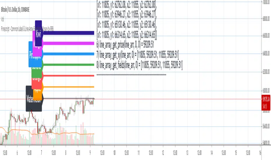
Fisher (zero-color + simple OB assist)//@version=5
indicator("Fisher (zero-color + simple OB assist)", overlay=false)
// Inputs
length = input.int(10, "Fisher Period", minval=1)
pivotLen = input.int(3, "Structure pivot length (SMC-lite)", minval=1)
showZero = input.bool(true, "Show Zero Line")
colPos = input.color(color.lime, "Color Above 0 (fallback)")
colNeg = input.color(color.red, "Color Below 0 (fallback)")
useOB = input.bool(true, "Color by OB proximity (Demand below = green, Supply above = red)")
showOBMarks = input.bool(true, "Show OB markers")
// Fisher (MT4-style port)
price = (high + low) / 2.0
hh = ta.highest(high, length)
ll = ta.lowest(low, length)
rng = hh - ll
norm = rng != 0 ? (price - ll) / rng : 0.5
var float v = 0.0
var float fish = 0.0
v := 0.33 * 2.0 * (norm - 0.5) + 0.67 * nz(v , 0)
v := math.min(math.max(v, -0.999), 0.999)
fish := 0.5 * math.log((1 + v) / (1 - v)) + 0.5 * nz(fish , 0)
// SMC-lite OB
ph = ta.pivothigh(high, pivotLen, pivotLen)
pl = ta.pivotlow(low, pivotLen, pivotLen)
var float lastSwingHigh = na
var float lastSwingLow = na
if not na(ph)
lastSwingHigh := ph
if not na(pl)
lastSwingLow := pl
bosUp = not na(lastSwingHigh) and close > lastSwingHigh
bosDn = not na(lastSwingLow) and close < lastSwingLow
bearishBar = close < open
bullishBar = close > open
demHigh_new = ta.valuewhen(bearishBar, high, 0)
demLow_new = ta.valuewhen(bearishBar, low, 0)
supHigh_new = ta.valuewhen(bullishBar, high, 0)
supLow_new = ta.valuewhen(bullishBar, low, 0)
// แยกประกาศตัวแปรทีละตัว และใช้ชนิดให้ชัดเจน
var float demHigh = na
var float demLow = na
var float supHigh = na
var float supLow = na
var bool demActive = false
var bool supActive = false
if bosUp and not na(demHigh_new) and not na(demLow_new)
demHigh := demHigh_new
demLow := demLow_new
demActive := true
if bosDn and not na(supHigh_new) and not na(supLow_new)
supHigh := supHigh_new
supLow := supLow_new
supActive := true
// Mitigation (แตะโซน)
if demActive and not na(demHigh) and not na(demLow)
if low <= demHigh
demActive := false
if supActive and not na(supHigh) and not na(supLow)
if high >= supLow
supActive := false
demandBelow = useOB and demActive and not na(demHigh) and demHigh <= close
supplyAbove = useOB and supActive and not na(supLow) and supLow >= close
colDimUp = color.new(colPos, 40)
colDimDown = color.new(colNeg, 40)
barColor = demandBelow ? colPos : supplyAbove ? colNeg : fish > 0 ? colDimUp : colDimDown
// Plots
plot(0, title="Zero", color=showZero ? color.new(color.gray, 70) : color.new(color.gray, 100))
plot(fish, title="Fisher", style=plot.style_columns, color=barColor, linewidth=2)
plotchar(showOBMarks and demandBelow ? fish : na, title="Demand below", char="D", location=location.absolute, color=color.teal, size=size.tiny)
plotchar(showOBMarks and supplyAbove ? fish : na, title="Supply above", char="S", location=location.absolute, color=color.fuchsia, size=size.tiny)
alertcondition(ta.crossover(fish, 0.0), "Fisher Cross Up", "Fisher crosses above 0")
alertcondition(ta.crossunder(fish, 0.0), "Fisher Cross Down", "Fisher crosses below 0")

Trend Lines by Pivots (Enhanced)### **📌 Detailed Explanation of the TradingView Indicator Code**
This **Pine Script v5** indicator automatically **detects trend lines** based on pivot highs and pivot lows. It helps traders visualize **support and resistance levels** using dynamic trend lines.
---
## **🔹 How the Indicator Works**
The indicator identifies **key pivot points** in price action and then **draws trend lines** connecting them. It works as follows:
1. **Detects Pivot Highs and Lows**:
- A **pivot high** is a local maximum where the price is higher than surrounding bars.
- A **pivot low** is a local minimum where the price is lower than surrounding bars.
2. **Stores the Last Two Pivot Points**:
- The script remembers the last **two pivot highs** and **two pivot lows**.
- These points are used to **draw resistance and support lines** dynamically.
3. **Plots Resistance and Support Lines**:
- The script continuously **updates** and **extends** the trend lines to the right as new pivots are found.
- **Red Line (Resistance):** Connects the last two pivot highs.
- **Green Line (Support):** Connects the last two pivot lows.
---
## **🔹 Code Breakdown**
### **1️⃣ Inputs for User Customization**
```pinescript
leftLen = input.int(2, "Left Pivot Length")
rightLen = input.int(2, "Right Pivot Length")
highLineColor = input.color(color.red, "Resistance Line Color")
lowLineColor = input.color(color.green, "Support Line Color")
```
- **leftLen & rightLen:** Define how many bars on the left and right should be used to confirm a pivot.
- **highLineColor:** Sets the color of the resistance trend line (default: **red**).
- **lowLineColor:** Sets the color of the support trend line (default: **green**).
---
### **2️⃣ Detect Pivot Highs & Lows**
```pinescript
pivotHigh = ta.pivothigh(leftLen, rightLen)
pivotLow = ta.pivotlow(leftLen, rightLen)
```
- `ta.pivothigh(leftLen, rightLen)`: Detects a **pivot high** if it's the highest price in a certain range.
- `ta.pivotlow(leftLen, rightLen)`: Detects a **pivot low** if it's the lowest price in a certain range.
---
### **3️⃣ Store the Last Two Pivot Points**
#### **🔺 Storing Resistance (Pivot Highs)**
```pinescript
var float lastPivotHigh1 = na
var int lastPivotHighIndex1 = na
var float lastPivotHigh2 = na
var int lastPivotHighIndex2 = na
```
- These variables store **the last two pivot highs** and their **bar indices** (position on the chart).
#### **🔻 Storing Support (Pivot Lows)**
```pinescript
var float lastPivotLow1 = na
var int lastPivotLowIndex1 = na
var float lastPivotLow2 = na
var int lastPivotLowIndex2 = na
```
- These variables store **the last two pivot lows** and their **bar indices**.
---
### **4️⃣ Update Pivot Points When New Ones Are Found**
#### **Updating Resistance (Pivot Highs)**
```pinescript
if not na(pivotHigh)
lastPivotHigh2 := lastPivotHigh1
lastPivotHighIndex2 := lastPivotHighIndex1
lastPivotHigh1 := pivotHigh
lastPivotHighIndex1 := bar_index - rightLen
```
- If a new **pivot high** is found:
- The **previous pivot** becomes `lastPivotHigh2`.
- The **new pivot** becomes `lastPivotHigh1`.
- The index (`bar_index - rightLen`) marks where the pivot occurred.
#### **Updating Support (Pivot Lows)**
```pinescript
if not na(pivotLow)
lastPivotLow2 := lastPivotLow1
lastPivotLowIndex2 := lastPivotLowIndex1
lastPivotLow1 := pivotLow
lastPivotLowIndex1 := bar_index - rightLen
```
- Similar to pivot highs, this section updates **pivot lows** dynamically.
---
### **5️⃣ Create and Update Trend Lines**
#### **🔺 Drawing the Resistance Line**
```pinescript
var line highLine = na
if not na(lastPivotHigh2) and not na(lastPivotHigh1)
if na(highLine)
highLine := line.new(lastPivotHighIndex2, lastPivotHigh2, lastPivotHighIndex1, lastPivotHigh1, color=highLineColor, extend=extend.right)
else
line.set_xy1(highLine, lastPivotHighIndex2, lastPivotHigh2)
line.set_xy2(highLine, lastPivotHighIndex1, lastPivotHigh1)
line.set_color(highLine, highLineColor)
```
- If **two pivot highs** exist:
- **First time:** Creates a new **resistance line** connecting them.
- **Updates dynamically:** Adjusts the line when a new pivot appears.
#### **🔻 Drawing the Support Line**
```pinescript
var line lowLine = na
if not na(lastPivotLow2) and not na(lastPivotLow1)
if na(lowLine)
lowLine := line.new(lastPivotLowIndex2, lastPivotLow2, lastPivotLowIndex1, lastPivotLow1, color=lowLineColor, extend=extend.right)
else
line.set_xy1(lowLine, lastPivotLowIndex2, lastPivotLow2)
line.set_xy2(lowLine, lastPivotLowIndex1, lastPivotLow1)
line.set_color(lowLine, lowLineColor)
```
- Same logic applies for **support levels**, creating or updating a **green trend line**.
---
## **🔹 How to Use This Indicator**
1. **Apply the script in TradingView**:
- Open **Pine Script Editor** → Paste the code → Click **"Add to Chart"**.
2. **Interpret the Lines**:
- **Red line (Resistance):** Price may struggle to break above it.
- **Green line (Support):** Price may bounce off it.
3. **Trading Strategy**:
- **Breakout Strategy:**
- If the price **breaks resistance**, expect a bullish move.
- If the price **breaks support**, expect a bearish move.
- **Reversal Trading:**
- Look for **bounces off support/resistance** for potential reversals.
---
## **🔹 Key Features of This Indicator**
✅ **Automatically detects pivot highs and lows.**
✅ **Draws real-time trend lines for support and resistance.**
✅ **Updates dynamically with new price action.**
✅ **Customizable settings for pivot sensitivity and colors.**
This indicator is useful for **trend traders, breakout traders, and support/resistance traders**. 🚀
Let me know if you need **further improvements or additional features!** 😊

Value At RiskThe Value at Risk Channel (VaR Channel) is a trading indicator designed to assist traders in managing their risk exposure effectively. By allowing users to select a specific time period and a probability value, this indicator generates upper and lower limits that the price might potentially attain within the chosen timeframe and probability range.
CONCEPTS
This indicator employs the concept of Value at Risk (VaR) calculation, a crucial metric in risk management. VaR quantifies the potential financial loss within a position, portfolio, or company over a defined time period. Financial institutions like banks and investment firms use VaR to estimate the extent and likelihood of potential losses in their portfolios.
The "historical method" is utilized to compute VaR within the indicator. This method analyzes the historical performance of returns and constructs a histogram representing the statistical distribution of past returns. Assuming returns adhere to a normal distribution, probabilities are assigned to different return values based on their position in the distribution percentile.
HOW TO USE
Suppose you wish to plot upper and lower price limits for a 4-hour period with a 5% probability. Access the indicator's Settings tab and set the Timeframe parameter to "4 hours" while configuring the Probability parameter to 5.0.
The indicator serves as a tool to determine appropriate Stop-Loss levels triggering with low probability. Additionally, it helps gauge the likelihood of triggering such levels.
Likewise, you can assess the probability of your desired Take-Profit level being reached within a specified time frame. For instance, if you anticipate your target to be achieved within a week, set the Timeframe parameter to "1 week" and adjust the Probability parameter to align the VaR channel's limits with your Take-Profit level. The resulting Probability parameter value reflects the likelihood of your target being met within the expected time frame.
This indicator proves valuable for evaluating and managing risk, as well as refining trading strategies. If you discover other applications for this indicator, feel free to share them in the comments!
SETTINGS
Timeframe: Designates the time period within which the price might touch the VaR channel's upper or lower boundary, considering the specified Probability parameter.
Probability: Defines the likelihood of the price reaching the VaR channel's upper or lower limit during the timeframe determined by the Timeframe parameter.
Window: Establishes the historical period (number of past bars) utilized for VaR calculation.

Pinescript v3 Compatibility Framework (v4 Migration Tool)Pinescript v3 Compatibility Framework (v4 Migration Tool)
This code makes most v3 scripts work in v4 with only a few minor changes below. Place the framework code before the first input statement.
You can totally delete all comments.
Pros:
- to port to v4 you only need to make a few simple changes, not affecting the core v3 code functionality
Cons:
- without #include - large redundant code block, but can be reduced as needed
- no proper syntax highlighting, intellisence for substitute constant names
Make the following changes in v3 script:
1. standard types can't be var names, color_transp can't be in a function, rename in v3 script:
color() => color.new()
bool => bool_
integer => integer_
float => float_
string => string_
2. init na requires explicit type declaration
float a = na
color col = na
3. persistent var init (optional):
s = na
s := nz(s , s) // or s := na(s ) ? 0 : s
// can be replaced with var s
var s = 0
s := s + 1
___________________________________________________________
Key features of Pinescript v4 (FYI):
1. optional explicit type declaration/conversion (you still can't cast series to int)
float s
2. persistent var modifier
var s
var float s
3. string series - persistent strings now can be used in cond and output to screen dynamically
4. label and line objects
- can be dynamically created, deleted, modified using get/set functions, moved before/after the current bar
- can be in if or a function unlike plot
- max limit: 50-55 label, and 50-55 line drawing objects in addition to already existing plots - both not affected by max plot outputs 64
- can only be used in the main chart
- can serve as the only output function - at least one is required: plot, barcolor, line, label etc.
- dynamic var values (including strings) can be output to screen as text using label.new and to_string
str = close >= open ? "up" : "down"
label.new(bar_index, high, text=str)
col = close >= open ? color.green : color.red
label.new(bar_index, na, "close = " + tostring(close), color=col, textcolor=color.white, style=label.style_labeldown, yloc=yloc.abovebar)
// create new objects, delete old ones
l = line.new(bar_index, high, bar_index , low , width=4)
line.delete(l )
// free object buffer by deleting old objects first, then create new ones
var l = na
line.delete(l)
l = line.new(bar_index, high, bar_index , low , width=4)

footprint_typeLibrary "footprint_type"
Contains all types for calculating and rendering footprints
Inputs
Inputs objects
Fields:
inbalance_percent (series int) : percentage coefficient to determine the Imbalance of price levels
stacked_input (series int) : minimum number of consecutive Imbalance levels required to draw extended lines
show_summary_footprint (series bool) : bool input for show summary footprint
procent_volume_area (series int) : definition size Value area
show_vah (series bool) : bool input for show VAH
show_poc (series bool) : bool input for show POC
show_val (series bool) : bool input for show VAL
color_vah (series color) : color VAH line
color_poc (series color) : color POC line
color_val (series color) : color VAL line
show_volume_profile (series bool)
new_imbalance_cond (series bool) : bool input for setup alert on new imbalance buy and sell
new_imbalance_line_cond (series bool) : bool input for setup alert on new imbalance line buy and sell
stop_past_imbalance_line_cond (series bool) : bool input for setup alert on stop past imbalance line buy and sell
Constants
Constants all Constants objects
Fields:
imbalance_high_char (series string) : char for printing buy imbalance
imbalance_low_char (series string) : char for printing sell imbalance
color_title_sell (series color) : color for footprint sell
color_title_buy (series color) : color for footprint buy
color_line_sell (series color) : color for sell line
color_line_buy (series color) : color for buy line
color_title_none (series color) : color None
Calculation_data
Calculation_data data for calculating
Fields:
detail_open (array) : array open from calculation timeframe
detail_high (array) : array high from calculation timeframe
detail_low (array) : array low from calculation timeframe
detail_close (array) : array close from calculation timeframe
detail_vol (array) : array volume from calculation timeframe
previos_detail_close (array) : array close from calculation timeframe
isBuyVolume (series bool) : attribute previosly bar buy or sell
Footprint_row
Footprint_row objects one footprint row
Fields:
price (series float) : row price
buy_vol (series float) : buy volume
sell_vol (series float) : sell volume
imbalance_buy (series bool) : attribute buy inbalance
imbalance_sell (series bool) : attribute sell imbalance
buy_vol_box (series box) : for ptinting buy volume
sell_vol_box (series box) : for printing sell volume
buy_vp_box (series box) : for ptinting volume profile buy
sell_vp_box (series box) : for ptinting volume profile sell
row_line (series label) : for ptinting row price
empty (series bool) : = true attribute row with zero volume buy and zero volume sell
Value_area
Value_area objects for calculating and printing Value area
Fields:
vah_price (series float) : VAH price
poc_price (series float) : POC price
val_price (series float) : VAL price
vah_label (series label) : label for VAH
poc_label (series label) : label for POC
val_label (series label) : label for VAL
vah_line (series line) : line for VAH
poc_level (series line) : line for POC
val_line (series line) : line for VAL
Imbalance_line_var_object
Imbalance_line_var_object var objects printing and calculation imbalance line
Fields:
cum_buy_line (array) : line array for saving all history buy imbalance line
cum_sell_line (array) : line array for saving all history sell imbalance line
Imbalance_line
Imbalance_line objects printing and calculation imbalance line
Fields:
buy_price_line (array) : float array for saving buy imbalance price level
sell_price_line (array) : float array for saving sell imbalance price level
var_imba_line (Imbalance_line_var_object) : var objects this type
Footprint_info_var_object
Footprint_info_var_object var objects for info printing
Fields:
cum_delta (series float) : var delta volume
cum_total (series float) : var total volume
cum_buy_vol (series float) : var buy volume
cum_sell_vol (series float) : var sell volume
cum_info (series table) : table for ptinting
Footprint_info
Footprint_info objects for info printing
Fields:
var_info (Footprint_info_var_object) : var objects this type
total (series label) : total volume
delta (series label) : delta volume
summary_label (series label) : label for ptinting
Footprint_bar
Footprint_bar all objects one bar with footprint
Fields:
foot_rows (array) : objects one row footprint
val_area (Value_area) : objects Value area
imba_line (Imbalance_line) : objects imbalance line
info (Footprint_info) : objects info - table,label and their variable
row_size (series float) : size rows
total_vol (series float) : total volume one footprint bar
foot_buy_vol (series float) : buy volume one footprint bar
foot_sell_vol (series float) : sell volume one footprint bar
foot_max_price_vol (map) : map with one value - price row with max volume buy + sell
calc_data (Calculation_data) : objects with detail data from calculation resolution
Support_objects
Support_objects support object for footprint calculation
Fields:
consts (Constants) : all consts objects
inp (Inputs) : all input objects
bar_index_show_condition (series bool) : calculation bool value for show all objects footprint
row_line_color (series color) : calculation value - color for row price

Polyline PlusThis library introduces the `PolylinePlus` type, which is an enhanced version of the built-in PineScript `polyline`. It enables two features that are absent from the built-in type:
1. Developers can now efficiently add or remove points from the polyline. In contrast, the built-in `polyline` type is immutable, requiring developers to create a new instance of the polyline to make changes, which is cumbersome and incurs a significant performance penalty.
2. Each `PolylinePlus` instance can theoretically hold up to ~1M points, surpassing the built-in `polyline` type's limit of 10K points, as long as it does not exceed the memory limit of the PineScript runtime.
Internally, each `PolylinePlus` instance utilizes an array of `line`s and an array of `polyline`s. The `line`s array serves as a buffer to store lines formed by recently added points. When the buffer reaches its capacity, it flushes the contents and converts the lines into polylines. These polylines are expected to undergo fewer updates. This approach is similiar to the concept of "Buffered I/O" in file and network systems. By connecting the underlying lines and polylines, this library achieves an enhanced polyline that is dynamic, efficient, and capable of surpassing the maximum number of points imposed by the built-in polyline.
🔵 API
Step 1: Import this library
import algotraderdev/polylineplus/1 as pp
// remember to check the latest version of this library and replace the 1 above.
Step 2: Initialize the `PolylinePlus` type.
var p = pp.PolylinePlus.new()
There are a few optional params that developers can specify in the constructor to modify the behavior and appearance of the polyline instance.
var p = pp.PolylinePlus.new(
// If true, the drawing will also connect the first point to the last point, resulting in a closed polyline.
closed = false,
// Determines the field of the chart.point objects that the polyline will use for its x coordinates. Either xloc.bar_index (default), or xloc.bar_time.
xloc = xloc.bar_index,
// Color of the polyline. Default is blue.
line_color = color.blue,
// Style of the polyline. Default is line.style_solid.
line_style = line.style_solid,
// Width of the polyline. Default is 1.
line_width = 1,
// The maximum number of points that each built-in `polyline` instance can contain.
// NOTE: this is not to be confused with the maximum of points that each `PolylinePlus` instance can contain.
max_points_per_builtin_polyline = 10000,
// The number of lines to keep in the buffer. If more points are to be added while the buffer is full, then all the lines in the buffer will be flushed into the poylines.
// The higher the number, the less frequent we'll need to // flush the buffer, and thus lead to better performance.
// NOTE: the maximum total number of lines per chart allowed by PineScript is 500. But given there might be other places where the indicator or strategy are drawing lines outside this polyline context, the default value is 50 to be safe.
lines_bffer_size = 50)
Step 3: Push / Pop Points
// Push a single point
p.push_point(chart.point.now())
// Push multiple points
chart.point points = array.from(p1, p2, p3) // Where p1, p2, p3 are all chart.point type.
p.push_points(points)
// Pop point
p.pop_point()
// Resets all the points in the polyline.
p.set_points(points)
// Deletes the polyline.
p.delete()
🔵 Benchmark
Below is a simple benchmark comparing the performance between `PolylinePlus` and the native `polyline` type for incrementally adding 10K points to a polyline.
import algotraderdev/polylineplus/2 as pp
var t1 = 0
var t2 = 0
if bar_index < 10000
int start = timenow
var p = pp.PolylinePlus.new(xloc = xloc.bar_time, closed = true)
p.push_point(chart.point.now())
t1 += timenow - start
start := timenow
var polyline pl = na
var points = array.new()
points.push(chart.point.now())
if not na(pl)
pl.delete()
pl := polyline.new(points)
t2 += timenow - start
if barstate.islast
log.info('{0} {1}', t1, t2)
For this benchmark, `PolylinePlus` took ~300ms, whereas the native `polyline` type took ~6000ms.
We can also fine-tune the parameters for `PolylinePlus` to have a larger buffer size for `line`s and a smaller buffer for `polyline`s.
var p = pp.PolylinePlus.new(xloc = xloc.bar_time, closed = true, lines_buffer_size = 500, max_points_per_builtin_polyline = 1000)
With the above optimization, it only took `PolylinePlus` ~80ms to process the same 10K points, which is ~75x the performance compared to the native `polyline`.
