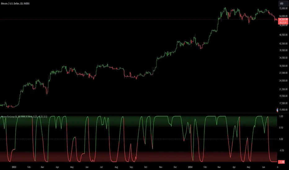
Aroon ForLoop [InvestorUnknown]Overview
The Aroon ForLoop indicator is designed to calculate an array of Aroon values over a range of lengths, providing trend signals based on various moving averages. It offers flexibility with different signal modes and visual customizations.
User Input
Start Length (a) and End Length (b): Defines the range for calculating Aroon values.
MA Type (maType) and MA Length (c): Selects the moving average type (EMA, SMA, WMA, VWMA, TMA) and its length.
Calculation Source (s): Specifies the data source for calculations.
Signal Mode (sigmode): Offers options like Fast, Slow, Thresholds Crossing, and Fast Threshold to generate signals.
Thresholds: Configures long and short thresholds for signal generation.
Visualization Options: Customizes bull and bear colors, and enables/disables bar coloring.
Alert Settings: Chooses whether to wait for bar close for alert confirmation.
Signal Calculation
Signal Mode (sigmode): Determines the type of signal generated by the indicator. Options are "Fast", "Slow", "Thresholds Crossing", and "Fast Threshold".
1. Slow: is a simple crossing of the midline (0).
2. Fast: positive signal depends if the current MA > MA or MA is above 0.99, negative signals comes if MA < MA or MA is below -0.99.
3. Thresholds Crossing: simple ta.crossover and ta.crossunder of the user defined threshold for Long and Short.
4. Fast Threshold: signal changes if the value of Aroon MA changes by more than user defined threshold against the current signal
col1 = MA > 0 ? colup : coldn
var color col2 = na
if MA > MA or MA > 0.99
col2 := colup
if MA < MA or MA < -0.99
col2 := coldn
var color col3 = na
if ta.crossover(MA,longth)
col3 := colup
if ta.crossunder(MA,shortth)
col3 := coldn
var color col4 = na
if (MA > MA + fastth)
col4 := colup
if (MA < MA - fastth)
col4 := coldn
color col = na
if sigmode == "Slow"
col := col1
if sigmode == "Fast"
col := col2
if sigmode == "Thresholds Crossing"
col := col3
if sigmode == "Fast Threshold"
col := col4
else
na
Visualization Settings
Bull Color (colup): The color used to indicate bullish signals.
Bear Color (coldn): The color used to indicate bearish signals.
Color Bars (barcol): Option to color the bars based on the signal.
Custom Function
AroonForLoop: Calculates Aroon values over the specified range, determines the trend, and averages the results using the chosen moving average type.
AroonForLoop(a, b, c) =>
var SignalArray = array.new_float(b - a + 1, 0.0)
for x = 0 to (b - a)
len = a + x
upper = 100 * (ta.highestbars(high, len + 1) + len)/len
lower = 100 * (ta.lowestbars(low, len + 1) + len)/len
trend = upper > lower ? 1 : -1
array.set(SignalArray, x, trend)
Avg = array.avg(SignalArray)
float MA = switch maType
"EMA" => ta.ema(Avg, c)
"SMA" => ta.sma(Avg, c)
"WMA" => ta.wma(Avg, c)
"VWMA" => ta.vwma(Avg, c)
"TMA" => ta.trima(Avg, c)
=>
runtime.error("No matching MA type found.")
float(na)
Important Considerations
Fast Responses: The Aroon ForLoop indicator is designed for quick identification of trend changes, making it ideal for fast-paced trading environments.
Moving Average Types: Supports various MA types (EMA, SMA, WMA, VWMA, TMA) for adaptable smoothing of trend signals.
Combination with Other Indicators: For more reliable signals, use this indicator in conjunction with other technical indicators.
Поиск скриптов по запросу "VAR+计量模型+黄金期货"
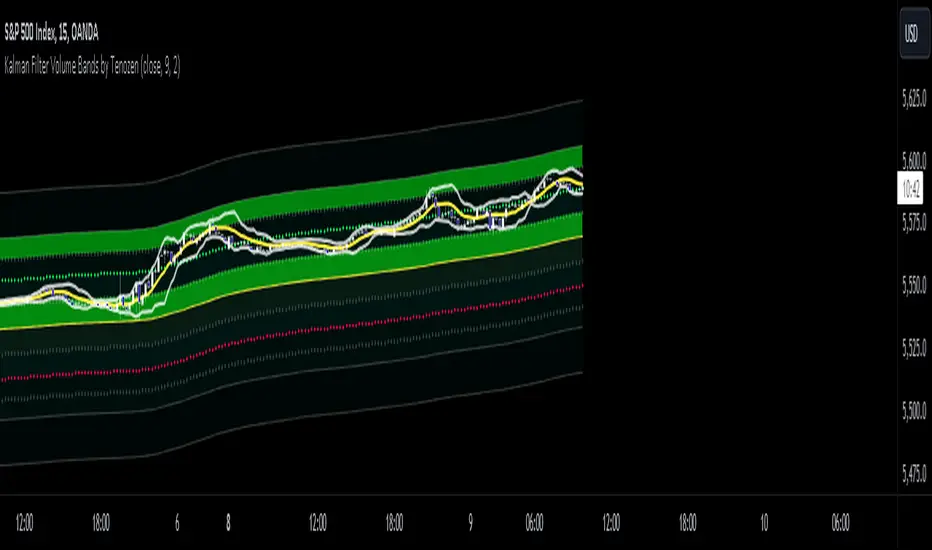
Kalman Filter Volume Bands by TenozenHello there! I am excited to introduce a new original indicator, the Kalman Filter Volume Bands. This indicator is calculated using the Kalman Filter, which is an adaptive-based smoothing quantitative tool. The Kalman Filter Volume Bands have two components that support the calculation, namely VWAP and VaR.
VWAP is used to determine the weight of the Kalman Filter Returns, but it doesn't have a significant impact on the calculation. On the other hand, VaR or Value at risk is calculated using the 99th percentile, which means that there is a 1% chance for the returns to exceed the 99th percentile level. After getting the VaR value, I manually adjust the bands based on the current market I'm trading on. I take the highest point (VaR*2) and the lowest point (-(VaR*2)) from the Kalman Filter, and then divide them into segments manually based on my preference.
This process results in 8 segments, where 2 segments near the Kalman Filter are further divided, making a total of 12 segments. These segments classify the current state of the price based on code-based coloring. The five states are very bullish, bullish, very bearish, bearish, and neutral.
I created this indicator to have an adaptive band that is not biased toward the volatility of the market. Most band-based indicators don't capture reversals that well, but the Kalman Filter Volume Bands can capture both trends and reversals. This makes it suitable for both trend-following and reversal trading approaches.
That's all for the explanation! Ciao!
Additional Reminder:
- Please use hourly timeframes or higher as lower timeframes are too noisy for reliable readings of this indicator.
ConditionalAverages█ OVERVIEW
This library is a Pine Script™ programmer’s tool containing functions that average values selectively.
█ CONCEPTS
Averaging can be useful to smooth out unstable readings in the data set, provide a benchmark to see the underlying trend of the data, or to provide a general expectancy of values in establishing a central tendency. Conventional averaging techniques tend to apply indiscriminately to all values in a fixed window, but it can sometimes be useful to average values only when a specific condition is met. As conditional averaging works on specific elements of a dataset, it can help us derive more context-specific conclusions. This library offers a collection of averaging methods that not only accomplish these tasks, but also exploit the efficiencies of the Pine Script™ runtime by foregoing unnecessary and resource-intensive for loops.
█ NOTES
To Loop or Not to Loop
Though for and while loops are essential programming tools, they are often unnecessary in Pine Script™. This is because the Pine Script™ runtime already runs your scripts in a loop where it executes your code on each bar of the dataset. Pine Script™ programmers who understand how their code executes on charts can use this to their advantage by designing loop-less code that will run orders of magnitude faster than functionally identical code using loops. Most of this library's function illustrate how you can achieve loop-less code to process past values. See the User Manual page on loops for more information. If you are looking for ways to measure execution time for you scripts, have a look at our LibraryStopwatch library .
Our `avgForTimeWhen()` and `totalForTimeWhen()` are exceptions in the library, as they use a while structure. Only a few iterations of the loop are executed on each bar, however, as its only job is to remove the few elements in the array that are outside the moving window defined by a time boundary.
Cumulating and Summing Conditionally
The ta.cum() or math.sum() built-in functions can be used with ternaries that select only certain values. In our `avgWhen(src, cond)` function, for example, we use this technique to cumulate only the occurrences of `src` when `cond` is true:
float cumTotal = ta.cum(cond ? src : 0) We then use:
float cumCount = ta.cum(cond ? 1 : 0) to calculate the number of occurrences where `cond` is true, which corresponds to the quantity of values cumulated in `cumTotal`.
Building Custom Series With Arrays
The advent of arrays in Pine has enabled us to build our custom data series. Many of this library's functions use arrays for this purpose, saving newer values that come in when a condition is met, and discarding the older ones, implementing a queue .
`avgForTimeWhen()` and `totalForTimeWhen()`
These two functions warrant a few explanations. They operate on a number of values included in a moving window defined by a timeframe expressed in milliseconds. We use a 1D timeframe in our example code. The number of bars included in the moving window is unknown to the programmer, who only specifies the period of time defining the moving window. You can thus use `avgForTimeWhen()` to calculate a rolling moving average for the last 24 hours, for example, that will work whether the chart is using a 1min or 1H timeframe. A 24-hour moving window will typically contain many more values on a 1min chart that on a 1H chart, but their calculated average will be very close.
Problems will arise on non-24x7 markets when large time gaps occur between chart bars, as will be the case across holidays or trading sessions. For example, if you were using a 24H timeframe and there is a two-day gap between two bars, then no chart bars would fit in the moving window after the gap. The `minBars` parameter mitigates this by guaranteeing that a minimum number of bars are always included in the calculation, even if including those bars requires reaching outside the prescribed timeframe. We use a minimum value of 10 bars in the example code.
Using var in Constant Declarations
In the past, we have been using var when initializing so-called constants in our scripts, which as per the Style Guide 's recommendations, we identify using UPPER_SNAKE_CASE. It turns out that var variables incur slightly superior maintenance overhead in the Pine Script™ runtime, when compared to variables initialized on each bar. We thus no longer use var to declare our "int/float/bool" constants, but still use it when an initialization on each bar would require too much time, such as when initializing a string or with a heavy function call.
Look first. Then leap.
█ FUNCTIONS
avgWhen(src, cond)
Gathers values of the source when a condition is true and averages them over the total number of occurrences of the condition.
Parameters:
src : (series int/float) The source of the values to be averaged.
cond : (series bool) The condition determining when a value will be included in the set of values to be averaged.
Returns: (float) A cumulative average of values when a condition is met.
avgWhenLast(src, cond, cnt)
Gathers values of the source when a condition is true and averages them over a defined number of occurrences of the condition.
Parameters:
src : (series int/float) The source of the values to be averaged.
cond : (series bool) The condition determining when a value will be included in the set of values to be averaged.
cnt : (simple int) The quantity of last occurrences of the condition for which to average values.
Returns: (float) The average of `src` for the last `x` occurrences where `cond` is true.
avgWhenInLast(src, cond, cnt)
Gathers values of the source when a condition is true and averages them over the total number of occurrences during a defined number of bars back.
Parameters:
src : (series int/float) The source of the values to be averaged.
cond : (series bool) The condition determining when a value will be included in the set of values to be averaged.
cnt : (simple int) The quantity of bars back to evaluate.
Returns: (float) The average of `src` in last `cnt` bars, but only when `cond` is true.
avgSince(src, cond)
Averages values of the source since a condition was true.
Parameters:
src : (series int/float) The source of the values to be averaged.
cond : (series bool) The condition determining when the average is reset.
Returns: (float) The average of `src` since `cond` was true.
avgForTimeWhen(src, ms, cond, minBars)
Averages values of `src` when `cond` is true, over a moving window of length `ms` milliseconds.
Parameters:
src : (series int/float) The source of the values to be averaged.
ms : (simple int) The time duration in milliseconds defining the size of the moving window.
cond : (series bool) The condition determining which values are included. Optional.
minBars : (simple int) The minimum number of values to keep in the moving window. Optional.
Returns: (float) The average of `src` when `cond` is true in the moving window.
totalForTimeWhen(src, ms, cond, minBars)
Sums values of `src` when `cond` is true, over a moving window of length `ms` milliseconds.
Parameters:
src : (series int/float) The source of the values to be summed.
ms : (simple int) The time duration in milliseconds defining the size of the moving window.
cond : (series bool) The condition determining which values are included. Optional.
minBars : (simple int) The minimum number of values to keep in the moving window. Optional.
Returns: (float) The sum of `src` when `cond` is true in the moving window.

Logger Library For Pinescript (Logging and Debugging)Library "LoggerLib"
This is a logging library for Pinescript. It is aimed to help developers testing and debugging scripts with a simple to use logger function.
Pinescript lacks a native logging implementation. This library would be helpful to mitigate this insufficiency.
This library uses table to print outputs into its view. It is simple, customizable and robust.
You can start using it's .log() method just like any other logging method in other languages.
//////////////////
USAGE
//////////////////
-- Recommended: Please Read The Documentation From Source Code Below. It Is Much More Readable There And Will Be Updated Along With Newer Versions. --
Importing the Library
---------------------
import paragjyoti2012/LoggerLib/ as Logger
.init() : Initializes the library and returns the logger pointer. (Later will be used as a function parameter)
.initTable: Initializes the Table View for the Logger and returns the table id. (Later will be used as a function parameter)
parameters:
logger: The logger pointer got from .init()
max_rows_count: Number of Rows to display in the Logger Table (default is 10)
offset: The offset value for the rows (Used for scrolling the view)
position: Position of the Table View
Values could be:
left
right
top-right
(default is left)
size: Font Size of content
Values could be:
small
normal
large
(default is small)
hide_date: Whether to hide the Date/Time column in the Logger (default is false)
returns: Table
example usage of .initTable()
import paragjyoti2012/LoggerLib/1 as Logger
var logger=Logger.init()
var logTable=Logger.initTable(logger, max_rows_count=20, offset=0, position="top-right")
-------------------
LOGGING
-------------------
.log() : Logging Method
params: (string message, |string| logger, table table_id, string type="message")
logger: pass the logger pointer from .init()
table_id: pass the table pointer from .initTable()
message: The message to log
type: Type of the log message
Values could be:
message
warning
error
info
success
(default is message)
returns: void
///////////////////////////////////////
Full Boilerplate For Using In Indicator
///////////////////////////////////////
P.S: Change the | (pipe) character into square brackets while using in script (or copy it from the source code instead)
offset=input.int(0,"Offset",minval=0)
size=input.string("small","Font Size",options=|"normal","small","large"|)
rows=input.int(15,"No Of Rows")
position=input.string("left","Position",options=|"left","right","top-right"|)
hide_date=input.bool(false,"Hide Time")
import paragjyoti2012/LoggerLib/1 as Logger
var logger=Logger.init()
var logTable=Logger.initTable(logger,rows,offset,position,size,hide_date)
rsi=ta.rsi(close,14)
|macd,signal,hist|=ta.macd(close,12,26,9)
if(ta.crossunder(close,34000))
Logger.log("Dropped Below 34000",logger,logTable,"warning")
if(ta.crossunder(close,35000))
Logger.log("Dropped Below 35000",logger,logTable)
if(ta.crossover(close,38000))
Logger.log("Crossed 38000",logger,logTable,"info")
if(ta.crossunder(rsi,20))
Logger.log("RSI Below 20",logger,logTable,"error")
if(ta.crossover(macd,signal))
Logger.log("Macd Crossed Over Signal",logger,logTable)
if(ta.crossover(rsi,80))
Logger.log("RSI Above 80",logger,logTable,"success")
////////////////////////////
// For Scrolling the Table View
////////////////////////////
There is a subtle way of achieving nice scrolling behaviour for the Table view. Open the input properties panel for the table/indicator. Focus on the input field for "Offset", once it's focused, you could use your mouse scroll wheel to increment/decrement the offset values; It will smoothly scroll the Logger Table Rows as well.
/////////////////////
For any assistance using this library or reporting issues, please write in the comment section below.
I will try my best to guide you and update the library. Thanks :)
/////////////////////

[BCT] Can BTC be predicted or is it purely random?Variance Ratio**This indicator can be applied to the ticker of your choice (not just BTC)**
Markets are said to be "efficient". An efficient market is by definition unpredictable - no matter the amount of ML, computation, or indicators thrown at it. In particular, in an efficient market, TA will not be of help.
An illustration of efficient markets is the WSJ's longstanding monkey vs. human contest:Blindfolded Monkey Beats Humans With Stock Picks, granted there are several flaws to it.
BTC is a relatively new market. New markets are typically highly inefficient (easier to make money) and become more and more efficient over time (harder to make money). How much more efficient is BTC becoming?
We apply the Variance Ratio method and apply it to BTC.
BACKGROUND ON THE VARIANCE RATIO METHOD
Based on 1988 MacKinlay's seminal paper "Stock Market Prices do not Follow a Random Walk", the idea is to exploit a phenomenon called "variance scaling".
For those keen on looking into the math, the short version of it is under the assumption of iid (random walk) we have the following:
H0: Var(Sum(returns over K bars))=Sum(Var(returns over 1 bar))=k*Var(return over 1 bar)
We look to reject or not H0 depending on the observations.
In this script, we compare the variance of the (log) returns for the chart selected between:
(1) The (average) variance over k bars (call this Vk)
(2) The (average) variance over 1 bar (call this V1)
H0 simply says that Vk=k*V1 if the stock follows a random walk.
We compute the Variance Ratio VR(k)=Variance(returns over k bar)/(Sum(Var(returns over 1 bar)))-1
We then compute the associated Z-score which we chart out for a configurable k number of bars.
HOW TO INTERPRET THE CHART
The line drawn is the Z-Score for VR(k). It represents the number of standard deviations of VR(k) from 0 - the further out, the less random.
- If the line is close / hovers around 0, the ticker appears to follow a random walk (i.e. may not be predictable)
- If the line is consistently > 2 or <-2, the ticker likely does not follow a random walk (i.e. may have predictable features)
- If the line is positive, it means that the Variance on the k bars is larger than the variance on 1 bar (more variance on longer timeframes)
- If the line is negative, it means that the Variance on the k bars is smaller than the variance on 1 bar (more variance on smaller timeframes)
USE CASES
- Identify timeframes where you won't be able to make money
- Identify whether a stock cannot be predicted (forget about TA, indicators etc. -- a random walk is not predictable)
- Identify whether a stock is becoming less and less predictable (Z-score amplitude will decrease over time)
FEATURES
- select the number of K bar to compare vs. 1 bar (default = 16) - ideally a power of 2 but any other number will work. The chart is based off this selection
- select the lookback period for the analysis (500 bars by default)
- select the source to analyze (default = close, but you may select other inputs to calculate the returns from)
- results form the statistical tests on different K's in the table on the right/bottom side of the chart (H0 rejected = not random walk; H0 not rejected = it essentially looks rather random and we can't conclude that it's not a random walk)
COMMENTARY ON BTC
- It appears BTC's absolute value of the ZScore on the Variance Ratio is declining year after year - corroborating an increasingly efficient market as new participants join.
- However, we can still detect a fair amount of potential inefficiency using this simple test.
As usual, this is not investment advice. DYOR.
With love,
🐵BCT🐵

Two Poles Trend Finder MTF [BigBeluga]🔵 OVERVIEW
Two Poles Trend Finder MTF is a refined trend-following overlay that blends a two-pole Gaussian filter with a multi-timeframe dashboard. It provides a smooth view of price dynamics along with a clear summary of trend directions across multiple timeframes—perfect for traders seeking alignment between short and long-term momentum.
🔵 CONCEPTS
Two-Pole Filter: A smoothing algorithm that responds faster than traditional moving averages but avoids the noise of short-term fluctuations.
var float f = na
var float f_prev1 = na
var float f_prev2 = na
// Apply two-pole Gaussian filter
if bar_index >= 2
f := math.pow(alpha, 2) * source + 2 * (1 - alpha) * f_prev1 - math.pow(1 - alpha, 2) * f_prev2
else
f := source // Warm-up for first bars
// Shift state
f_prev2 := f_prev1
f_prev1 := f
Trend Detection Logic: Trend direction is determined by comparing the current filtered value with its value n bars ago (shifted comparison).
MTF Alignment Dashboard: Trends from 5 configurable timeframes are monitored and visualized as colored boxes:
• Green = Uptrend
• Magenta = Downtrend
Summary Arrow: An average trend score from all timeframes is used to plot an overall arrow next to the asset name.
🔵 FEATURES
Two-Pole Gaussian Filter offers ultra-smooth trend curves while maintaining responsiveness.
Multi-Timeframe Trend Detection:
• Default: 1H, 2H, 4H, 12H, 1D (fully customizable)
• Each timeframe is assessed independently using the same trend logic.
Visual Trend Dashboard positioned at the bottom-right of the chart with color-coded trend blocks.
Dynamic Summary Arrow shows overall market bias (🢁 / 🢃) based on majority of uptrends/downtrends.
Bold + wide trail plot for the filter value with gradient coloring based on directional bias.
🔵 HOW TO USE
Use the multi-timeframe dashboard to identify aligned trends across your preferred trading horizons.
Confirm trend strength or weakness by observing filter slope direction .
Look for dashboard consensus (e.g., 4 or more timeframes green] ) as confirmation for breakout, continuation, or trend reentry strategies.
Combine with volume or price structure to enhance entry timing.
🔵 CONCLUSION
Two Poles Trend Finder MTF delivers a clean and intuitive trend-following solution with built-in multi-timeframe awareness. Whether you’re trading intra-day or positioning for swing setups, this tool helps filter out market noise and keeps you focused on directional consensus.

light_logLight Log - A Defensive Programming Library for Pine Script
Overview
The Light Log library transforms Pine Script development by introducing structured logging and defensive programming patterns typically found in enterprise languages like C#. This library addresses a fundamental challenge in Pine Script: the lack of sophisticated error handling and debugging tools that developers expect when building complex trading systems.
At its core, Light Log provides three transformative capabilities that work together to create more reliable and maintainable code. First, it wraps all native Pine Script types in error-aware containers, allowing values to carry validation state alongside their data. Second, it offers a comprehensive logging system with severity levels and conditional rendering. Third, it includes defensive programming utilities that catch errors early and make code self-documenting.
The Philosophy of Errors as Values
Traditional Pine Script error handling relies on runtime errors that halt execution, making it difficult to build resilient systems that can gracefully handle edge cases. Light Log introduces a paradigm shift by treating errors as first-class values that flow through your program alongside regular data.
When you wrap a value using Light Log's type system, you're not just storing data – you're creating a container that can carry both the value and its validation state. For example, when you call myNumber.INT() , you receive an INT object that contains both the integer value and a Log object that can describe any issues with that value. This approach, inspired by functional programming languages, allows errors to propagate through calculations without causing immediate failures.
Consider how this changes error handling in practice. Instead of a calculation failing catastrophically when it encounters invalid input, it can produce a result object that contains both the computed value (which might be na) and a detailed log explaining what went wrong. Subsequent operations can check has_error() to decide whether to proceed or handle the error condition gracefully.
The Typed Wrapper System
Light Log provides typed wrappers for every native Pine Script type: INT, FLOAT, BOOL, STRING, COLOR, LINE, LABEL, BOX, TABLE, CHART_POINT, POLYLINE, and LINEFILL. These wrappers serve multiple purposes beyond simple value storage.
Each wrapper type contains two fields: the value field v holds the actual data, while the error field e contains a Log object that tracks the value's validation state. This dual nature enables powerful programming patterns. You can perform operations on wrapped values and accumulate error information along the way, creating an audit trail of how values were processed.
The wrapper system includes convenient methods for converting between wrapped and unwrapped values. The extension methods like INT() , FLOAT() , etc., make it easy to wrap existing values, while the from_INT() , from_FLOAT() methods extract the underlying values when needed. The has_error() method provides a consistent interface for checking whether any wrapped value has encountered issues during processing.
The Log Object: Your Debugging Companion
The Log object represents the heart of Light Log's debugging capabilities. Unlike simple string concatenation for error messages, the Log object provides a structured approach to building, modifying, and rendering diagnostic information.
Each Log object carries three essential pieces of information: an error type (info, warning, error, or runtime_error), a message string that can be built incrementally, and an active flag that controls conditional rendering. This structure enables sophisticated logging patterns where you can build up detailed diagnostic information throughout your script's execution and decide later whether and how to display it.
The Log object's methods support fluent chaining, allowing you to build complex messages in a readable way. The write() and write_line() methods append text to the log, while new_line() adds formatting. The clear() method resets the log for reuse, and the rendering methods ( render_now() , render_condition() , and the general render() ) control when and how messages appear.
Defensive Programming Made Easy
Light Log's argument validation functions transform how you write defensive code. Instead of cluttering your functions with verbose validation logic, you can use concise, self-documenting calls that make your intentions clear.
The argument_error() function provides strict validation that halts execution when conditions aren't met – perfect for catching programming errors early. For less critical issues, argument_log_warning() and argument_log_error() record problems without stopping execution, while argument_log_info() provides debug visibility into your function's behavior.
These functions follow a consistent pattern: they take a condition to check, the function name, the argument name, and a descriptive message. This consistency makes error messages predictable and helpful, automatically formatting them to show exactly where problems occurred.
Building Modular, Reusable Code
Light Log encourages a modular approach to Pine Script development by providing tools that make functions more self-contained and reliable. When functions validate their inputs and return wrapped values with error information, they become true black boxes that can be safely composed into larger systems.
The void_return() function addresses Pine Script's requirement that all code paths return a value, even in error handling branches. This utility function provides a clean way to satisfy the compiler while making it clear that a particular code path should never execute.
The static log pattern, initialized with init_static_log() , enables module-wide error tracking. You can create a persistent Log object that accumulates information across multiple function calls, building a comprehensive diagnostic report that helps you understand complex behaviors in your indicators and strategies.
Real-World Applications
In practice, Light Log shines when building sophisticated trading systems. Imagine developing a complex indicator that processes multiple data streams, performs statistical calculations, and generates trading signals. With Light Log, each processing stage can validate its inputs, perform calculations, and pass along both results and diagnostic information.
For example, a moving average calculation might check that the period is positive, that sufficient data exists, and that the input series contains valid values. Instead of failing silently or throwing runtime errors, it can return a FLOAT object that contains either the calculated average or a detailed explanation of why the calculation couldn't be performed.
Strategy developers benefit even more from Light Log's capabilities. Complex entry and exit logic often involves multiple conditions that must all be satisfied. With Light Log, each condition check can contribute to a comprehensive log that explains exactly why a trade was or wasn't taken, making strategy debugging and optimization much more straightforward.
Performance Considerations
While Light Log adds a layer of abstraction over raw Pine Script values, its design minimizes performance impact. The wrapper objects are lightweight, containing only two fields. The logging operations only consume resources when actually rendered, and the conditional rendering system ensures that production code can run with logging disabled for maximum performance.
The library follows Pine Script best practices for performance, using appropriate data structures and avoiding unnecessary operations. The var keyword in init_static_log() ensures that persistent logs don't create new objects on every bar, maintaining efficiency even in real-time calculations.
Getting Started
Adopting Light Log in your Pine Script projects is straightforward. Import the library, wrap your critical values, add validation to your functions, and use Log objects to track important events. Start small by adding logging to a single function, then expand as you see the benefits of better error visibility and code organization.
Remember that Light Log is designed to grow with your needs. You can use as much or as little of its functionality as makes sense for your project. Even simple uses, like adding argument validation to key functions, can significantly improve code reliability and debugging ease.
Transform your Pine Script development experience with Light Log – because professional trading systems deserve professional development tools.
Light Log Technical Deep Dive: Advanced Patterns and Architecture
Understanding Errors as Values
The concept of "errors as values" represents a fundamental shift in how we think about error handling in Pine Script. In traditional Pine Script development, errors are events – they happen at a specific moment in time and immediately interrupt program flow. Light Log transforms errors into data – they become information that flows through your program just like any other value.
This transformation has profound implications. When errors are values, they can be stored, passed between functions, accumulated, transformed, and inspected. They become part of your program's data flow rather than exceptions to it. This approach, popularized by languages like Rust with its Result type and Haskell with its Either monad, brings functional programming's elegance to Pine Script.
Consider a practical example. Traditional Pine Script might calculate a momentum indicator like this:
momentum = close - close
If period is invalid or if there isn't enough historical data, this calculation might produce na or cause subtle bugs. With Light Log's approach:
calculate_momentum(src, period)=>
result = src.FLOAT()
if period <= 0
result.e.write("Invalid period: must be positive", true, ErrorType.error)
result.v := na
else if bar_index < period
result.e.write("Insufficient data: need " + str.tostring(period) + " bars", true, ErrorType.warning)
result.v := na
else
result.v := src - src
result.e.write("Momentum calculated successfully", false, ErrorType.info)
result
Now the function returns not just a value but a complete computational result that includes diagnostic information. Calling code can make intelligent decisions based on both the value and its associated metadata.
The Monad Pattern in Pine Script
While Pine Script lacks the type system features to implement true monads, Light Log brings monadic thinking to Pine Script development. The wrapped types (INT, FLOAT, etc.) act as computational contexts that carry both values and metadata through a series of transformations.
The key insight of monadic programming is that you can chain operations while automatically propagating context. In Light Log, this context is the error state. When you have a FLOAT that contains an error, operations on that FLOAT can check the error state and decide whether to proceed or propagate the error.
This pattern enables what functional programmers call "railway-oriented programming" – your code follows a success track when all is well but can switch to an error track when problems occur. Both tracks lead to the same destination (a result with error information), but they take different paths based on the validity of intermediate values.
Composable Error Handling
Light Log's design encourages composition – building complex functionality from simpler, well-tested components. Each component can validate its inputs, perform its calculation, and return a result with appropriate error information. Higher-level functions can then combine these results intelligently.
Consider building a complex trading signal from multiple indicators:
generate_signal(src, fast_period, slow_period, signal_period) =>
log = init_static_log(ErrorType.info)
// Calculate components with error tracking
fast_ma = calculate_ma(src, fast_period)
slow_ma = calculate_ma(src, slow_period)
// Check for errors in components
if fast_ma.has_error()
log.write_line("Fast MA error: " + fast_ma.e.message, true)
if slow_ma.has_error()
log.write_line("Slow MA error: " + slow_ma.e.message, true)
// Proceed with calculation if no errors
signal = 0.0.FLOAT()
if not (fast_ma.has_error() or slow_ma.has_error())
macd_line = fast_ma.v - slow_ma.v
signal_line = calculate_ma(macd_line, signal_period)
if signal_line.has_error()
log.write_line("Signal line error: " + signal_line.e.message, true)
signal.e := log
else
signal.v := macd_line - signal_line.v
log.write("Signal generated successfully")
else
signal.e := log
signal.v := na
signal
This composable approach makes complex calculations more reliable and easier to debug. Each component is responsible for its own validation and error reporting, and the composite function orchestrates these components while maintaining comprehensive error tracking.
The Static Log Pattern
The init_static_log() function introduces a powerful pattern for maintaining state across function calls. In Pine Script, the var keyword creates variables that persist across bars but are initialized only once. Light Log leverages this to create logging objects that can accumulate information throughout a script's execution.
This pattern is particularly valuable for debugging complex strategies where you need to understand behavior across multiple bars. You can create module-level logs that track important events:
// Module-level diagnostic log
diagnostics = init_static_log(ErrorType.info)
// Track strategy decisions across bars
check_entry_conditions() =>
diagnostics.clear() // Start fresh each bar
diagnostics.write_line("Bar " + str.tostring(bar_index) + " analysis:")
if close > sma(close, 20)
diagnostics.write_line("Price above SMA20", false)
else
diagnostics.write_line("Price below SMA20 - no entry", true, ErrorType.warning)
if volume > sma(volume, 20) * 1.5
diagnostics.write_line("Volume surge detected", false)
else
diagnostics.write_line("Normal volume", false)
// Render diagnostics based on verbosity setting
if debug_mode
diagnostics.render_now()
Advanced Validation Patterns
Light Log's argument validation functions enable sophisticated precondition checking that goes beyond simple null checks. You can implement complex validation logic while keeping your code readable:
validate_price_data(open_val, high_val, low_val, close_val) =>
argument_error(na(open_val) or na(high_val) or na(low_val) or na(close_val),
"validate_price_data", "OHLC values", "contain na values")
argument_error(high_val < low_val,
"validate_price_data", "high/low", "high is less than low")
argument_error(close_val > high_val or close_val < low_val,
"validate_price_data", "close", "is outside high/low range")
argument_log_warning(high_val == low_val,
"validate_price_data", "high/low", "are equal (no range)")
This validation function documents its requirements clearly and fails fast with helpful error messages when assumptions are violated. The mix of errors (which halt execution) and warnings (which allow continuation) provides fine-grained control over how strict your validation should be.
Performance Optimization Strategies
While Light Log adds abstraction, careful design minimizes overhead. Understanding Pine Script's execution model helps you use Light Log efficiently.
Pine Script executes once per bar, so operations that seem expensive in traditional programming might have negligible impact. However, when building real-time systems, every optimization matters. Light Log provides several patterns for efficient use:
Lazy Evaluation: Log messages are only built when they'll be rendered. Use conditional logging to avoid string concatenation in production:
if debug_mode
log.write_line("Calculated value: " + str.tostring(complex_calculation))
Selective Wrapping: Not every value needs error tracking. Wrap values at API boundaries and critical calculation points, but use raw values for simple operations:
// Wrap at boundaries
input_price = close.FLOAT()
validated_period = validate_period(input_period).INT()
// Use raw values internally
sum = 0.0
for i = 0 to validated_period.v - 1
sum += close
Error Propagation: When errors occur early, avoid expensive calculations:
process_data(input) =>
validated = validate_input(input)
if validated.has_error()
validated // Return early with error
else
// Expensive processing only if valid
perform_complex_calculation(validated)
Integration Patterns
Light Log integrates smoothly with existing Pine Script code. You can adopt it incrementally, starting with critical functions and expanding coverage as needed.
Boundary Validation: Add Light Log at the boundaries of your system – where user input enters and where final outputs are produced. This catches most errors while minimizing changes to existing code.
Progressive Enhancement: Start by adding argument validation to existing functions. Then wrap return values. Finally, add comprehensive logging. Each step improves reliability without requiring a complete rewrite.
Testing and Debugging: Use Light Log's conditional rendering to create debug modes for your scripts. Production users see clean output while developers get detailed diagnostics:
// User input for debug mode
debug = input.bool(false, "Enable debug logging")
// Conditional diagnostic output
if debug
diagnostics.render_now()
else
diagnostics.render_condition() // Only shows errors/warnings
Future-Proofing Your Code
Light Log's patterns prepare your code for Pine Script's evolution. As Pine Script adds more sophisticated features, code that uses structured error handling and defensive programming will adapt more easily than code that relies on implicit assumptions.
The type wrapper system, in particular, positions your code to take advantage of potential future features or more sophisticated type inference. By thinking in terms of wrapped values and error propagation today, you're building code that will remain maintainable and extensible tomorrow.
Light Log doesn't just make your Pine Script better today – it prepares it for the trading systems you'll need to build tomorrow.
Library "light_log"
A lightweight logging and defensive programming library for Pine Script.
Designed for modular and extensible scripts, this utility provides structured runtime validation,
conditional logging, and reusable `Log` objects for centralized error propagation.
It also introduces a typed wrapping system for all native Pine values (e.g., `INT`, `FLOAT`, `LABEL`),
allowing values to carry errors alongside data. This enables functional-style flows with built-in
validation tracking, error detection (`has_error()`), and fluent chaining.
Inspired by structured logging patterns found in systems like C#, it reduces boilerplate,
enforces argument safety, and encourages clean, maintainable code architecture.
method INT(self, error_type)
Wraps an `int` value into an `INT` struct with an optional log severity.
Namespace types: series int, simple int, input int, const int
Parameters:
self (int) : The raw `int` value to wrap.
error_type (series ErrorType) : Optional severity level to associate with the log. Default is `ErrorType.error`.
Returns: An `INT` object containing the value and a default Log instance.
method FLOAT(self, error_type)
Wraps a `float` value into a `FLOAT` struct with an optional log severity.
Namespace types: series float, simple float, input float, const float
Parameters:
self (float) : The raw `float` value to wrap.
error_type (series ErrorType) : Optional severity level to associate with the log. Default is `ErrorType.error`.
Returns: A `FLOAT` object containing the value and a default Log instance.
method BOOL(self, error_type)
Wraps a `bool` value into a `BOOL` struct with an optional log severity.
Namespace types: series bool, simple bool, input bool, const bool
Parameters:
self (bool) : The raw `bool` value to wrap.
error_type (series ErrorType) : Optional severity level to associate with the log. Default is `ErrorType.error`.
Returns: A `BOOL` object containing the value and a default Log instance.
method STRING(self, error_type)
Wraps a `string` value into a `STRING` struct with an optional log severity.
Namespace types: series string, simple string, input string, const string
Parameters:
self (string) : The raw `string` value to wrap.
error_type (series ErrorType) : Optional severity level to associate with the log. Default is `ErrorType.error`.
Returns: A `STRING` object containing the value and a default Log instance.
method COLOR(self, error_type)
Wraps a `color` value into a `COLOR` struct with an optional log severity.
Namespace types: series color, simple color, input color, const color
Parameters:
self (color) : The raw `color` value to wrap.
error_type (series ErrorType) : Optional severity level to associate with the log. Default is `ErrorType.error`.
Returns: A `COLOR` object containing the value and a default Log instance.
method LINE(self, error_type)
Wraps a `line` object into a `LINE` struct with an optional log severity.
Namespace types: series line
Parameters:
self (line) : The raw `line` object to wrap.
error_type (series ErrorType) : Optional severity level to associate with the log. Default is `ErrorType.error`.
Returns: A `LINE` object containing the value and a default Log instance.
method LABEL(self, error_type)
Wraps a `label` object into a `LABEL` struct with an optional log severity.
Namespace types: series label
Parameters:
self (label) : The raw `label` object to wrap.
error_type (series ErrorType) : Optional severity level to associate with the log. Default is `ErrorType.error`.
Returns: A `LABEL` object containing the value and a default Log instance.
method BOX(self, error_type)
Wraps a `box` object into a `BOX` struct with an optional log severity.
Namespace types: series box
Parameters:
self (box) : The raw `box` object to wrap.
error_type (series ErrorType) : Optional severity level to associate with the log. Default is `ErrorType.error`.
Returns: A `BOX` object containing the value and a default Log instance.
method TABLE(self, error_type)
Wraps a `table` object into a `TABLE` struct with an optional log severity.
Namespace types: series table
Parameters:
self (table) : The raw `table` object to wrap.
error_type (series ErrorType) : Optional severity level to associate with the log. Default is `ErrorType.error`.
Returns: A `TABLE` object containing the value and a default Log instance.
method CHART_POINT(self, error_type)
Wraps a `chart.point` value into a `CHART_POINT` struct with an optional log severity.
Namespace types: chart.point
Parameters:
self (chart.point) : The raw `chart.point` value to wrap.
error_type (series ErrorType) : Optional severity level to associate with the log. Default is `ErrorType.error`.
Returns: A `CHART_POINT` object containing the value and a default Log instance.
method POLYLINE(self, error_type)
Wraps a `polyline` object into a `POLYLINE` struct with an optional log severity.
Namespace types: series polyline, series polyline, series polyline, series polyline
Parameters:
self (polyline) : The raw `polyline` object to wrap.
error_type (series ErrorType) : Optional severity level to associate with the log. Default is `ErrorType.error`.
Returns: A `POLYLINE` object containing the value and a default Log instance.
method LINEFILL(self, error_type)
Wraps a `linefill` object into a `LINEFILL` struct with an optional log severity.
Namespace types: series linefill
Parameters:
self (linefill) : The raw `linefill` object to wrap.
error_type (series ErrorType) : Optional severity level to associate with the log. Default is `ErrorType.error`.
Returns: A `LINEFILL` object containing the value and a default Log instance.
method from_INT(self)
Extracts the integer value from an INT wrapper.
Namespace types: INT
Parameters:
self (INT) : The wrapped INT instance.
Returns: The underlying `int` value.
method from_FLOAT(self)
Extracts the float value from a FLOAT wrapper.
Namespace types: FLOAT
Parameters:
self (FLOAT) : The wrapped FLOAT instance.
Returns: The underlying `float` value.
method from_BOOL(self)
Extracts the boolean value from a BOOL wrapper.
Namespace types: BOOL
Parameters:
self (BOOL) : The wrapped BOOL instance.
Returns: The underlying `bool` value.
method from_STRING(self)
Extracts the string value from a STRING wrapper.
Namespace types: STRING
Parameters:
self (STRING) : The wrapped STRING instance.
Returns: The underlying `string` value.
method from_COLOR(self)
Extracts the color value from a COLOR wrapper.
Namespace types: COLOR
Parameters:
self (COLOR) : The wrapped COLOR instance.
Returns: The underlying `color` value.
method from_LINE(self)
Extracts the line object from a LINE wrapper.
Namespace types: LINE
Parameters:
self (LINE) : The wrapped LINE instance.
Returns: The underlying `line` object.
method from_LABEL(self)
Extracts the label object from a LABEL wrapper.
Namespace types: LABEL
Parameters:
self (LABEL) : The wrapped LABEL instance.
Returns: The underlying `label` object.
method from_BOX(self)
Extracts the box object from a BOX wrapper.
Namespace types: BOX
Parameters:
self (BOX) : The wrapped BOX instance.
Returns: The underlying `box` object.
method from_TABLE(self)
Extracts the table object from a TABLE wrapper.
Namespace types: TABLE
Parameters:
self (TABLE) : The wrapped TABLE instance.
Returns: The underlying `table` object.
method from_CHART_POINT(self)
Extracts the chart.point from a CHART_POINT wrapper.
Namespace types: CHART_POINT
Parameters:
self (CHART_POINT) : The wrapped CHART_POINT instance.
Returns: The underlying `chart.point` value.
method from_POLYLINE(self)
Extracts the polyline object from a POLYLINE wrapper.
Namespace types: POLYLINE
Parameters:
self (POLYLINE) : The wrapped POLYLINE instance.
Returns: The underlying `polyline` object.
method from_LINEFILL(self)
Extracts the linefill object from a LINEFILL wrapper.
Namespace types: LINEFILL
Parameters:
self (LINEFILL) : The wrapped LINEFILL instance.
Returns: The underlying `linefill` object.
method has_error(self)
Returns true if the INT wrapper has an active log entry.
Namespace types: INT
Parameters:
self (INT) : The INT instance to check.
Returns: True if an error or message is active in the log.
method has_error(self)
Returns true if the FLOAT wrapper has an active log entry.
Namespace types: FLOAT
Parameters:
self (FLOAT) : The FLOAT instance to check.
Returns: True if an error or message is active in the log.
method has_error(self)
Returns true if the BOOL wrapper has an active log entry.
Namespace types: BOOL
Parameters:
self (BOOL) : The BOOL instance to check.
Returns: True if an error or message is active in the log.
method has_error(self)
Returns true if the STRING wrapper has an active log entry.
Namespace types: STRING
Parameters:
self (STRING) : The STRING instance to check.
Returns: True if an error or message is active in the log.
method has_error(self)
Returns true if the COLOR wrapper has an active log entry.
Namespace types: COLOR
Parameters:
self (COLOR) : The COLOR instance to check.
Returns: True if an error or message is active in the log.
method has_error(self)
Returns true if the LINE wrapper has an active log entry.
Namespace types: LINE
Parameters:
self (LINE) : The LINE instance to check.
Returns: True if an error or message is active in the log.
method has_error(self)
Returns true if the LABEL wrapper has an active log entry.
Namespace types: LABEL
Parameters:
self (LABEL) : The LABEL instance to check.
Returns: True if an error or message is active in the log.
method has_error(self)
Returns true if the BOX wrapper has an active log entry.
Namespace types: BOX
Parameters:
self (BOX) : The BOX instance to check.
Returns: True if an error or message is active in the log.
method has_error(self)
Returns true if the TABLE wrapper has an active log entry.
Namespace types: TABLE
Parameters:
self (TABLE) : The TABLE instance to check.
Returns: True if an error or message is active in the log.
method has_error(self)
Returns true if the CHART_POINT wrapper has an active log entry.
Namespace types: CHART_POINT
Parameters:
self (CHART_POINT) : The CHART_POINT instance to check.
Returns: True if an error or message is active in the log.
method has_error(self)
Returns true if the POLYLINE wrapper has an active log entry.
Namespace types: POLYLINE
Parameters:
self (POLYLINE) : The POLYLINE instance to check.
Returns: True if an error or message is active in the log.
method has_error(self)
Returns true if the LINEFILL wrapper has an active log entry.
Namespace types: LINEFILL
Parameters:
self (LINEFILL) : The LINEFILL instance to check.
Returns: True if an error or message is active in the log.
void_return()
Utility function used when a return is syntactically required but functionally unnecessary.
Returns: Nothing. Function never executes its body.
argument_error(condition, function, argument, message)
Throws a runtime error when a condition is met. Used for strict argument validation.
Parameters:
condition (bool) : Boolean expression that triggers the runtime error.
function (string) : Name of the calling function (for formatting).
argument (string) : Name of the problematic argument.
message (string) : Description of the error cause.
Returns: Never returns. Halts execution if the condition is true.
argument_log_info(condition, function, argument, message)
Logs an informational message when a condition is met. Used for optional debug visibility.
Parameters:
condition (bool) : Boolean expression that triggers the log.
function (string) : Name of the calling function.
argument (string) : Argument name being referenced.
message (string) : Informational message to log.
Returns: Nothing. Logs if the condition is true.
argument_log_warning(condition, function, argument, message)
Logs a warning when a condition is met. Non-fatal but highlights potential issues.
Parameters:
condition (bool) : Boolean expression that triggers the warning.
function (string) : Name of the calling function.
argument (string) : Argument name being referenced.
message (string) : Warning message to log.
Returns: Nothing. Logs if the condition is true.
argument_log_error(condition, function, argument, message)
Logs an error message when a condition is met. Does not halt execution.
Parameters:
condition (bool) : Boolean expression that triggers the error log.
function (string) : Name of the calling function.
argument (string) : Argument name being referenced.
message (string) : Error message to log.
Returns: Nothing. Logs if the condition is true.
init_static_log(error_type, message, active)
Initializes a persistent (var) Log object. Ideal for global logging in scripts or modules.
Parameters:
error_type (series ErrorType) : Initial severity level (required).
message (string) : Optional starting message string. Default value of ("").
active (bool) : Whether the log should be flagged active on initialization. Default value of (false).
Returns: A static Log object with the given parameters.
method new_line(self)
Appends a newline character to the Log message. Useful for separating entries during chained writes.
Namespace types: Log
Parameters:
self (Log) : The Log instance to modify.
Returns: The updated Log object with a newline appended.
method write(self, message, flag_active, error_type)
Appends a message to a Log object without a newline. Updates severity and active state if specified.
Namespace types: Log
Parameters:
self (Log) : The Log instance being modified.
message (string) : The text to append to the log.
flag_active (bool) : Whether to activate the log for conditional rendering. Default value of (false).
error_type (series ErrorType) : Optional override for the severity level. Default value of (na).
Returns: The updated Log object.
method write_line(self, message, flag_active, error_type)
Appends a message to a Log object, prefixed with a newline for clarity.
Namespace types: Log
Parameters:
self (Log) : The Log instance being modified.
message (string) : The text to append to the log.
flag_active (bool) : Whether to activate the log for conditional rendering. Default value of (false).
error_type (series ErrorType) : Optional override for the severity level. Default value of (na).
Returns: The updated Log object.
method clear(self, flag_active, error_type)
Clears a Log object’s message and optionally reactivates it. Can also update the error type.
Namespace types: Log
Parameters:
self (Log) : The Log instance being cleared.
flag_active (bool) : Whether to activate the log after clearing. Default value of (false).
error_type (series ErrorType) : Optional new error type to assign. If not provided, the previous type is retained. Default value of (na).
Returns: The cleared Log object.
method render_condition(self, flag_active, error_type)
Conditionally renders the log if it is active. Allows overriding error type and controlling active state afterward.
Namespace types: Log
Parameters:
self (Log) : The Log instance to evaluate and render.
flag_active (bool) : Whether to activate the log after rendering. Default value of (false).
error_type (series ErrorType) : Optional error type override. Useful for contextual formatting just before rendering. Default value of (na).
Returns: The updated Log object.
method render_now(self, flag_active, error_type)
Immediately renders the log regardless of `active` state. Allows overriding error type and active flag.
Namespace types: Log
Parameters:
self (Log) : The Log instance to render.
flag_active (bool) : Whether to activate the log after rendering. Default value of (false).
error_type (series ErrorType) : Optional error type override. Allows dynamic severity adjustment at render time. Default value of (na).
Returns: The updated Log object.
render(self, condition, flag_active, error_type)
Renders the log conditionally or unconditionally. Allows full control over render behavior.
Parameters:
self (Log) : The Log instance to render.
condition (bool) : If true, renders only if the log is active. If false, always renders. Default value of (false).
flag_active (bool) : Whether to activate the log after rendering. Default value of (false).
error_type (series ErrorType) : Optional error type override passed to the render methods. Default value of (na).
Returns: The updated Log object.
Log
A structured object used to store and render logging messages.
Fields:
error_type (series ErrorType) : The severity level of the message (from the ErrorType enum).
message (series string) : The text of the log message.
active (series bool) : Whether the log should trigger rendering when conditionally evaluated.
INT
A wrapped integer type with attached logging for validation or tracing.
Fields:
v (series int) : The underlying `int` value.
e (Log) : Optional log object describing validation status or error context.
FLOAT
A wrapped float type with attached logging for validation or tracing.
Fields:
v (series float) : The underlying `float` value.
e (Log) : Optional log object describing validation status or error context.
BOOL
A wrapped boolean type with attached logging for validation or tracing.
Fields:
v (series bool) : The underlying `bool` value.
e (Log) : Optional log object describing validation status or error context.
STRING
A wrapped string type with attached logging for validation or tracing.
Fields:
v (series string) : The underlying `string` value.
e (Log) : Optional log object describing validation status or error context.
COLOR
A wrapped color type with attached logging for validation or tracing.
Fields:
v (series color) : The underlying `color` value.
e (Log) : Optional log object describing validation status or error context.
LINE
A wrapped line object with attached logging for validation or tracing.
Fields:
v (series line) : The underlying `line` value.
e (Log) : Optional log object describing validation status or error context.
LABEL
A wrapped label object with attached logging for validation or tracing.
Fields:
v (series label) : The underlying `label` value.
e (Log) : Optional log object describing validation status or error context.
BOX
A wrapped box object with attached logging for validation or tracing.
Fields:
v (series box) : The underlying `box` value.
e (Log) : Optional log object describing validation status or error context.
TABLE
A wrapped table object with attached logging for validation or tracing.
Fields:
v (series table) : The underlying `table` value.
e (Log) : Optional log object describing validation status or error context.
CHART_POINT
A wrapped chart point with attached logging for validation or tracing.
Fields:
v (chart.point) : The underlying `chart.point` value.
e (Log) : Optional log object describing validation status or error context.
POLYLINE
A wrapped polyline object with attached logging for validation or tracing.
Fields:
v (series polyline) : The underlying `polyline` value.
e (Log) : Optional log object describing validation status or error context.
LINEFILL
A wrapped linefill object with attached logging for validation or tracing.
Fields:
v (series linefill) : The underlying `linefill` value.
e (Log) : Optional log object describing validation status or error context.
FvgPanel█ OVERVIEW
This library provides functionalities for creating and managing a display panel within a Pine Script™ indicator. Its primary purpose is to offer a structured way to present Fair Value Gap (FVG) information, specifically the nearest bullish and bearish FVG levels across different timeframes (Current, MTF, HTF), directly on the chart. The library handles the table's structure, header initialization, and dynamic cell content updates.
█ CONCEPTS
The core of this library revolves around presenting summarized FVG data in a clear, tabular format. Key concepts include:
FVG Data Aggregation and Display
The panel is designed to show at-a-glance information about the closest active FVG mitigation levels. It doesn't calculate these FVGs itself but relies on the main script to provide this data. The panel is structured with columns for timeframes (TF), Bullish FVGs, and Bearish FVGs, and rows for "Current" (LTF), "MTF" (Medium Timeframe), and "HTF" (High Timeframe).
The `panelData` User-Defined Type (UDT)
To facilitate the transfer of information to be displayed, the library defines a UDT named `panelData`. This structure is central to the library's operation and is designed to hold all necessary values for populating the panel's data cells for each relevant FVG. Its fields include:
Price levels for the nearest bullish and bearish FVGs for LTF, MTF, and HTF (e.g., `nearestBullMitLvl`, `nearestMtfBearMitLvl`).
Boolean flags to indicate if these FVGs are classified as "Large Volume" (LV) (e.g., `isNearestBullLV`, `isNearestMtfBearLV`).
Color information for the background and text of each data cell, allowing for conditional styling based on the FVG's status or proximity (e.g., `ltfBullBgColor`, `mtfBearTextColor`).
The design of `panelData` allows the main script to prepare all display-related data and styling cues in one object, which is then passed to the `updatePanel` function for rendering. This separation of data preparation and display logic keeps the library focused on its presentation task.
Visual Cues and Formatting
Price Formatting: Price levels are formatted to match the instrument's minimum tick size using an internal `formatPrice` helper function, ensuring consistent and accurate display.
Large FVG Icon: If an FVG is marked as a "Large Volume" FVG in the `panelData` object, a user-specified icon (e.g., an emoji) is prepended to its price level in the panel, providing an immediate visual distinction.
Conditional Styling: The background and text colors for each FVG level displayed in the panel can be individually controlled via the `panelData` object, enabling the main script to implement custom styling rules (e.g., highlighting the overall nearest FVG across all timeframes).
Handling Missing Data: If no FVG data is available for a particular cell (i.e., the corresponding level in `panelData` is `na`), the panel displays "---" and uses a specified background color for "Not Available" cells.
█ CALCULATIONS AND USE
Using the `FvgPanel` typically involves a two-stage process: initialization and dynamic updates.
Step 1: Panel Creation
First, an instance of the panel table is created once, usually during the script's initial setup. This is done using the `createPanel` function.
Call `createPanel()` with parameters defining its position on the chart, border color, border width, header background color, header text color, and header text size.
This function initializes the table with three columns ("TF", "Bull FVG", "Bear FVG") and three data rows labeled "Current", "MTF", and "HTF", plus a header row.
Store the returned `table` object in a `var` variable to persist it across bars.
// Example:
var table infoPanel = na
if barstate.isfirst
infoPanel := panel.createPanel(
position.top_right,
color.gray,
1,
color.new(color.gray, 50),
color.white,
size.small
)
Step 2: Panel Updates
On each bar, or whenever the FVG data changes (typically on `barstate.islast` or `barstate.isrealtime` for efficiency), the panel's content needs to be refreshed. This is done using the `updatePanel` function.
Populate an instance of the `panelData` UDT with the latest FVG information. This includes setting the nearest bullish/bearish mitigation levels for LTF, MTF, and HTF, their LV status, and their desired background and text colors.
Call `updatePanel()`, passing the persistent `table` object (from Step 1), the populated `panelData` object, the icon string for LV FVGs, the default text color for FVG levels, the background color for "N/A" cells, and the general text size for the data cells.
The `updatePanel` function will then clear previous data and fill the table cells with the new values and styles provided in the `panelData` object.
// Example (inside a conditional block like 'if barstate.islast'):
var panelData fvgDisplayData = panelData.new()
// ... (logic to populate fvgDisplayData fields) ...
// fvgDisplayData.nearestBullMitLvl = ...
// fvgDisplayData.ltfBullBgColor = ...
// ... etc.
if not na(infoPanel)
panel.updatePanel(
infoPanel,
fvgDisplayData,
"🔥", // LV FVG Icon
color.white,
color.new(color.gray, 70), // NA Cell Color
size.small
)
This workflow ensures that the panel is drawn only once and its cells are efficiently updated as new data becomes available.
█ NOTES
Data Source: This library is solely responsible for the visual presentation of FVG data in a table. It does not perform any FVG detection or calculation. The calling script must compute or retrieve the FVG levels, LV status, and desired styling to populate the `panelData` object.
Styling Responsibility: While `updatePanel` applies colors passed via the `panelData` object, the logic for *determining* those colors (e.g., highlighting the closest FVG to the current price) resides in the calling script.
Performance: The library uses `table.cell()` to update individual cells, which is generally more efficient than deleting and recreating the table on each update. However, the frequency of `updatePanel` calls should be managed by the main script (e.g., using `barstate.islast` or `barstate.isrealtime`) to avoid excessive processing on historical bars.
`series float` Handling: The price level fields within the `panelData` UDT (e.g., `nearestBullMitLvl`) can accept `series float` values, as these are typically derived from price data. The internal `formatPrice` function correctly handles `series float` for display.
Dependencies: The `FvgPanel` itself is self-contained and does not import other user libraries. It uses standard Pine Script™ table and string functionalities.
█ EXPORTED TYPES
panelData
Represents the data structure for populating the FVG information panel.
Fields:
nearestBullMitLvl (series float) : The price level of the nearest bullish FVG's mitigation point (bottom for bull) on the LTF.
isNearestBullLV (series bool) : True if the nearest bullish FVG on the LTF is a Large Volume FVG.
ltfBullBgColor (series color) : Background color for the LTF bullish FVG cell in the panel.
ltfBullTextColor (series color) : Text color for the LTF bullish FVG cell in the panel.
nearestBearMitLvl (series float) : The price level of the nearest bearish FVG's mitigation point (top for bear) on the LTF.
isNearestBearLV (series bool) : True if the nearest bearish FVG on the LTF is a Large Volume FVG.
ltfBearBgColor (series color) : Background color for the LTF bearish FVG cell in the panel.
ltfBearTextColor (series color) : Text color for the LTF bearish FVG cell in the panel.
nearestMtfBullMitLvl (series float) : The price level of the nearest bullish FVG's mitigation point on the MTF.
isNearestMtfBullLV (series bool) : True if the nearest bullish FVG on the MTF is a Large Volume FVG.
mtfBullBgColor (series color) : Background color for the MTF bullish FVG cell.
mtfBullTextColor (series color) : Text color for the MTF bullish FVG cell.
nearestMtfBearMitLvl (series float) : The price level of the nearest bearish FVG's mitigation point on the MTF.
isNearestMtfBearLV (series bool) : True if the nearest bearish FVG on the MTF is a Large Volume FVG.
mtfBearBgColor (series color) : Background color for the MTF bearish FVG cell.
mtfBearTextColor (series color) : Text color for the MTF bearish FVG cell.
nearestHtfBullMitLvl (series float) : The price level of the nearest bullish FVG's mitigation point on the HTF.
isNearestHtfBullLV (series bool) : True if the nearest bullish FVG on the HTF is a Large Volume FVG.
htfBullBgColor (series color) : Background color for the HTF bullish FVG cell.
htfBullTextColor (series color) : Text color for the HTF bullish FVG cell.
nearestHtfBearMitLvl (series float) : The price level of the nearest bearish FVG's mitigation point on the HTF.
isNearestHtfBearLV (series bool) : True if the nearest bearish FVG on the HTF is a Large Volume FVG.
htfBearBgColor (series color) : Background color for the HTF bearish FVG cell.
htfBearTextColor (series color) : Text color for the HTF bearish FVG cell.
█ EXPORTED FUNCTIONS
createPanel(position, borderColor, borderWidth, headerBgColor, headerTextColor, headerTextSize)
Creates and initializes the FVG information panel (table). Sets up the header rows and timeframe labels.
Parameters:
position (simple string) : The position of the panel on the chart (e.g., position.top_right). Uses position.* constants.
borderColor (simple color) : The color of the panel's border.
borderWidth (simple int) : The width of the panel's border.
headerBgColor (simple color) : The background color for the header cells.
headerTextColor (simple color) : The text color for the header cells.
headerTextSize (simple string) : The text size for the header cells (e.g., size.small). Uses size.* constants.
Returns: The newly created table object representing the panel.
updatePanel(panelTable, data, lvIcon, defaultTextColor, naCellColor, textSize)
Updates the content of the FVG information panel with the latest FVG data.
Parameters:
panelTable (table) : The table object representing the panel to be updated.
data (panelData) : An object containing the FVG data to display.
lvIcon (simple string) : The icon (e.g., emoji) to display next to Large Volume FVGs.
defaultTextColor (simple color) : The default text color for FVG levels if not highlighted.
naCellColor (simple color) : The background color for cells where no FVG data is available ("---").
textSize (simple string) : The text size for the FVG level data (e.g., size.small).
Returns: _void

XTE+ Optimized Trend Tracker📊 XTE+ Optimized Trend Tracker (OTT)
XTE+ OTT is a powerful, trend-following indicator designed for traders who value clarity, precision, and advanced analytics. It offers not only accurate entry and exit signals but also visual zones, historical signal analysis, and real-time trend monitoring.
🧠 How It Works
XTE+ OTT is based on an improved version of the Optimized Trend Tracker. It utilizes multiple customizable moving average types (VAR, EMA, SMA, WMA, and more) combined with volatility filtering (ATR logic) to generate cleaner, more reliable trend-following signals.
✅ Features
Trend Direction Detection with automatic switch logic
Buy/Sell Signal Icons with distinct large markers
Entry/Exit Zones drawn visually on chart
Custom Take-Profit / Stop-Loss settings for Buy and Sell signals
Statistical Panel showing:
Current Trend (Up/Down)
Number of total signals
Number of winning trades
Win percentage
Configurable Display Options:
Show/hide signals
Show/hide trend zones
Show/hide OTT and MA lines
Supports multiple MA types including EMA, SMA, VAR, ZLEMA, TSF and more
Non-repainting logic — signals are confirmed at bar close
⚙️ Inputs and Customization
OTT Period & Sensitivity (%)
MA Type Selection (VAR, EMA, etc.)
Entry Zone Visualization On/Off
Trend Panel Display On/Off
TP/SL % per direction (Buy/Sell separately)
Option to disable MA or OTT line display
📈 Visuals
Signal icons: BUY (Green Up Label), SELL (Red Down Label)
Entry zones: circles near breakout levels
Trendlines change color dynamically (green for uptrend, red for downtrend)
Trend Panel is pinned in the top-right corner for quick reference
💡 Usage Tips
Best used on higher timeframes (15min, 1H, 4H+) for more meaningful trend signals
Combine with volume/volatility indicators or support/resistance zones for enhanced decision making
Use TP/SL logic to track signal success over time and optimize strategies
📌 Disclaimer
This script is for educational and informational purposes only. It is not financial advice. Always test and validate your strategy before applying it in live markets.

SCE ReversalsThis tool uses past market data to attempt to identify where changes in “memory” may occur to spot reversals. The Hurst Exponent was a big inspiration for this code. The main driver is identifying when past ranges expand and contract, leading to a change in direction. With the use of Sum of Squared Errors, users do not need to input anything.
Getting optimized parameters
// Define ranges for N and lkb
N_range = array.from(15, 20, 25, 30, 35, 40, 45, 50, 55, 60)
// Function to calculate SSE
sse_calc(_N) =>
x = math.pow(close - close , 2)
y = math.pow(close - close , 2) + math.pow(close, 2)
z = x / y
scaled_z = z * math.log(_N)
min_r = ta.lowest(scaled_z, _N)
max_r = ta.highest(scaled_z, _N)
norm_r = (scaled_z - min_r) / (max_r - min_r)
SMA = ta.sma(close, _N)
reversal_bullish = norm_r == 1.000 and norm_r < 0.90 and close < SMA and session.ismarket and barstate.isconfirmed
reversal_bearish = norm_r == 1.000 and norm_r < 0.90 and close > SMA and session.ismarket and barstate.isconfirmed
var float error = na
if reversal_bullish or reversal_bearish
error := math.pow(close - SMA, 2)
error
else
error := 999999999999999999999999999999999999999
error
error
var int N_opt = na
var float min_SSE = na
// Loop through ranges and calculate SSE
for N in N_range
sse = sse_calc(N)
if na(min_SSE) or sse < min_SSE
min_SSE := sse
N_opt := N
The N_range list encompasses every lookback value to check with. The sse_calc function accepts an individual element to then perform the calculation for Reversals. If there is a reversal, the error becomes how far away the close is from a moving average with that look back. Lowest error wins. That would be the look back used for the Reversals calculation.
Reversals calculation
// Calculating with optimized parameters
x_opt = math.pow(close - close , 2)
y_opt = math.pow(close - close , 2) + math.pow(close, 2)
z_opt = x_opt / y_opt
scaled_z_opt = z_opt * math.log(N_opt)
min_r_opt = ta.lowest(scaled_z_opt, N_opt)
max_r_opt = ta.highest(scaled_z_opt, N_opt)
norm_r_opt = (scaled_z_opt - min_r_opt) / (max_r_opt - min_r_opt)
SMA_opt = ta.sma(close, N_opt)
reversal_bullish_opt = norm_r_opt == 1.000 and norm_r_opt < 0.90 and close < SMA_opt and close > high and close > open and session.ismarket and barstate.isconfirmed
reversal_bearish_opt = norm_r_opt == 1.000 and norm_r_opt < 0.90 and close > SMA_opt and close < low and close < open and session.ismarket and barstate.isconfirmed
X_opt and y_opt are the compared values to develop the system. Everything done afterwards is scaling and using it to spot the Reversals. X_opt is the current close, minus the close with the optimal N bars back, squared. Then y_opt is also that but plus the current close squared. Z_opt is then x_opt / y_opt. This gives us a pretty small number that will go up when we approach tops or bottoms. To make life a little easier I normalize the value between 0 and 1.
After I find the moving average with the optimal N, I can check if there is a Reversal. Reversals are there when the last value is at 1 and the current value drops below 0.90. This would tell us that “memory” was strong and is now changing. To determine direction and help with accuracy, if the close is above the moving average it is a bearish alert, and vice versa. As well as the close must be below the last low for a bearish Reversal, above the last high for a bullish Reversal. Also the close must be above the open for a bullish Reversal, and below for a bearish one.
Visual examples
This NASDAQ:TSLA chart shows how alerts may come around. The bullish and bearish labels are plotted on the chart along with a reference line to see price interact with.
The indicator has the potential to be inactive, like we see here on $OKLO. There is only one alert, and it marks the bottom nicely.
Stocks with strong trends like NYSE:NOW may be more susceptible to false alerts. Assets that are volatile and bounce around a lot may be better.
It works on intra day charts the same as on Daily or longer charts. We see here on NASDAQ:QQQ it spotted the bottom on this particular trading day.
This tool is meant to aid traders in making decisions, not to be followed blindly. No trading tool is 100% accurate and Sum of Squared Errors does not guarantee the most optimal value. I encourage feedback and constructive criticism.

20/50 SMA Cross 200 SMAThis Pine Script code is designed to identify and visualize crossovers of two shorter-term Simple Moving Averages (SMAs), a 20-period SMA and a 50-period SMA, with a longer-term 200-period SMA on a price chart. It also includes alerts for these crossover events. Here's a breakdown:
**Purpose:**
The core idea behind this script is to detect potential trend changes. Crossovers of shorter-term moving averages over a longer-term moving average are often interpreted as bullish signals, while crossovers below are considered bearish.
**Key Components:**
1. **Moving Average Calculation:**
* `sma20 = ta.sma(close, 20)`: Calculates the 20-period SMA of the closing price.
* `sma50 = ta.sma(close, 50)`: Calculates the 50-period SMA of the closing price.
* `sma200 = ta.sma(close, 200)`: Calculates the 200-period SMA of the closing price.
2. **Crossover Detection:**
* `crossUp20 = ta.crossover(sma20, sma200)`: Returns `true` when the 20-period SMA crosses above the 200-period SMA.
* `crossDown20 = ta.crossunder(sma20, sma200)`: Returns `true` when the 20-period SMA crosses below the 200-period SMA.
* Similar logic applies for `crossUp50` and `crossDown50` with the 50-period SMA.
3. **Recent Crossover Tracking (Crucial Improvement):**
* `lookback = 7`: Defines a lookback period of 7 bars.
* `var bool hasCrossedUp20 = false`, etc.: Declares `var` (persistent) boolean variables to track if a crossover has occurred *within* the last 7 bars. This is the most important correction from previous versions.
* The logic using `ta.barssince()` is the key:
* If a crossover happens (`crossUp20` is true), the corresponding `hasCrossedUp20` is set to `true`.
* If no crossover happens on the current bar, it checks if a crossover happened within the last 7 bars using `ta.barssince(crossUp20) <= lookback`. If so, it keeps `hasCrossedUp20` as `true`. After 7 bars, it becomes `false`.
4. **Plotting Crossovers:**
* `plotshape(...)`: Plots circles on the chart to visually mark the crossovers.
* Green circles below the bars for bullish crossovers (20 and 50).
* Red circles above the bars for bearish crossovers (20 and 50).
* Different shades of green/red (green/lime, red/maroon) distinguish between 20 and 50 SMA crossovers.
5. **Plotting Moving Averages (Optional but Helpful):**
* `plot(sma20, color=color.blue, linewidth=1)`: Plots the 20-period SMA in blue.
* Similar logic for the 50-period SMA (orange) and 200-period SMA (gray).
6. **Alerts:**
* `alertcondition(...)`: Triggers alerts when crossovers occur. This is essential for real-time trading signals.
**How it Works (in Simple Terms):**
The script continuously calculates the 20, 50, and 200 SMAs. It then monitors for instances where the 20 or 50 SMA crosses the 200 SMA. When such a crossover happens, a colored circle is plotted on the chart, and an alert is triggered. The key improvement is that it remembers if a crossover occurred in the last 7 bars and continues to display the circle during that period.
**Use Case:**
Traders use this type of indicator to identify potential entry and exit points in the market. A bullish crossover (shorter SMA crossing above the longer SMA) might be a signal to buy, while a bearish crossover might be a signal to sell.
**Key Improvements over Previous Versions:**
* **Correct Lookback Implementation:** The use of `ta.barssince()` and `var` variables is the correct and efficient way to check for crossovers within a lookback period. This fixes the major flaw in earlier versions.
* **Clear Visualizations:** The use of `plotshape` with distinct colors makes it easy to distinguish between 20 and 50 SMA crossovers.
* **Alerts:** The inclusion of alerts makes the script much more practical for real-time trading.
This improved version provides a robust and useful tool for identifying and tracking SMA crossovers.
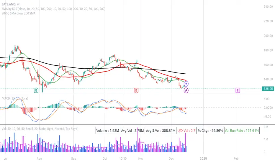
Cosine-Weighted MA ATR [InvestorUnknown]The Cosine-Weighted Moving Average (CWMA) ATR (Average True Range) indicator is designed to enhance the analysis of price movements in financial markets. By incorporating a cosine-based weighting mechanism , this indicator provides a unique approach to smoothing price data and measuring volatility, making it a valuable tool for traders and investors.
Cosine-Weighted Moving Average (CWMA)
The CWMA is calculated using weights derived from the cosine function, which emphasizes different data points in a distinctive manner. Unlike traditional moving averages that assign equal weight to all data points, the cosine weighting allocates more significance to values at the edges of the data window. This can help capture significant price movements while mitigating the impact of outlier values.
The weights are shifted to ensure they remain non-negative, which helps in maintaining a stable calculation throughout the data series. The normalization of these weights ensures they sum to one, providing a proportional contribution to the average.
// Function to calculate the Cosine-Weighted Moving Average with shifted weights
f_Cosine_Weighted_MA(series float src, simple int length) =>
var float cosine_weights = array.new_float(0)
array.clear(cosine_weights) // Clear the array before recalculating weights
for i = 0 to length - 1
weight = math.cos((math.pi * (i + 1)) / length) + 1 // Shift by adding 1
array.push(cosine_weights, weight)
// Normalize the weights
sum_weights = array.sum(cosine_weights)
for i = 0 to length - 1
norm_weight = array.get(cosine_weights, i) / sum_weights
array.set(cosine_weights, i, norm_weight)
// Calculate Cosine-Weighted Moving Average
cwma = 0.0
if bar_index >= length
for i = 0 to length - 1
cwma := cwma + array.get(cosine_weights, i) * close
cwma
Cosine-Weighted ATR Calculation
The ATR is an essential measure of volatility, reflecting the average range of price movement over a specified period. The Cosine-Weighted ATR uses a similar weighting scheme to that of the CWMA, allowing for a more nuanced understanding of volatility. By emphasizing more recent price movements while retaining sensitivity to broader trends, this ATR variant offers traders enhanced insight into potential price fluctuations.
// Function to calculate the Cosine-Weighted ATR with shifted weights
f_Cosine_Weighted_ATR(simple int length) =>
var float cosine_weights_atr = array.new_float(0)
array.clear(cosine_weights_atr)
for i = 0 to length - 1
weight = math.cos((math.pi * (i + 1)) / length) + 1 // Shift by adding 1
array.push(cosine_weights_atr, weight)
// Normalize the weights
sum_weights_atr = array.sum(cosine_weights_atr)
for i = 0 to length - 1
norm_weight_atr = array.get(cosine_weights_atr, i) / sum_weights_atr
array.set(cosine_weights_atr, i, norm_weight_atr)
// Calculate Cosine-Weighted ATR using true ranges
cwatr = 0.0
tr = ta.tr(true) // True Range
if bar_index >= length
for i = 0 to length - 1
cwatr := cwatr + array.get(cosine_weights_atr, i) * tr
cwatr
Signal Generation
The indicator generates long and short signals based on the relationship between the price (user input) and the calculated upper and lower bands, derived from the CWMA and the Cosine-Weighted ATR. Crossover conditions are used to identify potential entry points, providing a systematic approach to trading decisions.
// - - - - - CALCULATIONS - - - - - //{
bar b = bar.new()
float src = b.calc_src(cwma_src)
float cwma = f_Cosine_Weighted_MA(src, ma_length)
// Use normal ATR or Cosine-Weighted ATR based on input
float atr = atr_type == "Normal ATR" ? ta.atr(atr_len) : f_Cosine_Weighted_ATR(atr_len)
// Calculate upper and lower bands using ATR
float cwma_up = cwma + (atr * atr_mult)
float cwma_dn = cwma - (atr * atr_mult)
float src_l = b.calc_src(src_long)
float src_s = b.calc_src(src_short)
// Signal logic for crossovers and crossunders
var int signal = 0
if ta.crossover(src_l, cwma_up)
signal := 1
if ta.crossunder(src_s, cwma_dn)
signal := -1
//}
Backtest Mode and Equity Calculation
To evaluate its effectiveness, the indicator includes a backtest mode, allowing users to test its performance on historical data:
Backtest Equity: A detailed equity curve is calculated based on the generated signals over a user-defined period (startDate to endDate).
Buy and Hold Comparison: Alongside the strategy’s equity, a Buy-and-Hold equity curve is plotted for performance comparison.
Visualization and Alerts
The indicator features customizable plots, allowing users to visualize the CWMA, ATR bands, and signals effectively. The colors change dynamically based on market conditions, with clear distinctions between long and short signals.
Alerts can be configured to notify users of crossover events, providing timely information for potential trading opportunities.

Sine-Weighted MA ATR [InvestorUnknown]The Sine-Weighted MA ATR is a technical analysis tool designed to emphasize recent price data using sine-weighted calculations , making it particularly well-suited for analyzing cyclical markets with repetitive patterns . The indicator combines the Sine-Weighted Moving Average (SWMA) and a Sine-Weighted Average True Range (SWATR) to enhance price trend detection and volatility analysis.
Sine-Weighted Moving Average (SWMA):
Unlike traditional moving averages that apply uniform or exponentially decaying weights, the SWMA applies Sine weights to the price data.
Emphasis on central data points: The Sine function assigns more weight to the middle of the lookback period, giving less importance to the beginning and end points. This helps capture the main trend more effectively while reducing noise from recent volatility or older data.
// Function to calculate the Sine-Weighted Moving Average
f_Sine_Weighted_MA(series float src, simple int length) =>
var float sine_weights = array.new_float(0)
array.clear(sine_weights) // Clear the array before recalculating weights
for i = 0 to length - 1
weight = math.sin((math.pi * (i + 1)) / length)
array.push(sine_weights, weight)
// Normalize the weights
sum_weights = array.sum(sine_weights)
for i = 0 to length - 1
norm_weight = array.get(sine_weights, i) / sum_weights
array.set(sine_weights, i, norm_weight)
// Calculate Sine-Weighted Moving Average
swma = 0.0
if bar_index >= length
for i = 0 to length - 1
swma := swma + array.get(sine_weights, i) * close
swma
Sine-Weighted ATR:
This is a variation of the Average True Range (ATR), which measures market volatility. Like the SWMA, the ATR is smoothed using Sine-based weighting, where central values are more heavily considered compared to the extremities. This improves sensitivity to changes in volatility while maintaining stability in highly volatile markets.
// Function to calculate the Sine-Weighted ATR
f_Sine_Weighted_ATR(simple int length) =>
var float sine_weights_atr = array.new_float(0)
array.clear(sine_weights_atr)
for i = 0 to length - 1
weight = math.sin((math.pi * (i + 1)) / length)
array.push(sine_weights_atr, weight)
// Normalize the weights
sum_weights_atr = array.sum(sine_weights_atr)
for i = 0 to length - 1
norm_weight_atr = array.get(sine_weights_atr, i) / sum_weights_atr
array.set(sine_weights_atr, i, norm_weight_atr)
// Calculate Sine-Weighted ATR using true ranges
swatr = 0.0
tr = ta.tr(true) // True Range
if bar_index >= length
for i = 0 to length - 1
swatr := swatr + array.get(sine_weights_atr, i) * tr
swatr
ATR Bands:
Upper and lower bands are created by adding/subtracting the Sine-Weighted ATR from the SWMA. These bands help identify overbought or oversold conditions, and when the price crosses these levels, it may generate long or short trade signals.
// - - - - - CALCULATIONS - - - - - //{
bar b = bar.new()
float src = b.calc_src(swma_src)
float swma = f_Sine_Weighted_MA(src, ma_length)
// Use normal ATR or Sine-Weighted ATR based on input
float atr = atr_type == "Normal ATR" ? ta.atr(atr_len) : f_Sine_Weighted_ATR(atr_len)
// Calculate upper and lower bands using ATR
float swma_up = swma + (atr * atr_mult)
float swma_dn = swma - (atr * atr_mult)
float src_l = b.calc_src(src_long)
float src_s = b.calc_src(src_short)
// Signal logic for crossovers and crossunders
var int signal = 0
if ta.crossover(src_l, swma_up)
signal := 1
if ta.crossunder(src_s, swma_dn)
signal := -1
//}
Signal Logic:
Long/Short Signals are triggered when the price crosses above or below the Sine-Weighted ATR bands
Backtest Mode and Equity Calculation
To evaluate its effectiveness, the indicator includes a backtest mode, allowing users to test its performance on historical data:
Backtest Equity: A detailed equity curve is calculated based on the generated signals over a user-defined period (startDate to endDate).
Buy and Hold Comparison: Alongside the strategy’s equity, a Buy-and-Hold equity curve is plotted for performance comparison.
Alerts
The indicator includes built-in alerts for both long and short signals, ensuring users are promptly notified when market conditions meet the criteria for an entry or exit.

Bitcoin Thermocap [InvestorUnknown]The Bitcoin Thermocap indicator is designed to analyze Bitcoin's market data using a variant of the "Thermocap Multiple" concept from BitBo. This indicator offers several modes for interpreting Bitcoin's historical block and price data, aiding investors and analysts in understanding long-term market dynamics and generating potential investing signals.
Key Features:
1. Thermocap Calculation
The core of the indicator is based on the Thermocap Multiple, which evaluates Bitcoin's value relative to its cumulative historical blocks mined.
Thermocap Formula:
Source: Bitbo
btc_price = request.security("INDEX:BTCUSD", "1D", close)
BTC_BLOCKSMINED = request.security("BTC_BLOCKSMINED", "D", close)
// Variable to store the cumulative historical blocks
var float historical_blocks = na
// Initialize historical blocks on the first bar
if (na(historical_blocks))
historical_blocks := 0.0
// Update the cumulative blocks for each day
historical_blocks += BTC_BLOCKSMINED * btc_price
// Calculate the Thermocap
float thermocap = ((btc_price / historical_blocks) * 1000000) // the multiplication is just for better visualization
2. Multiple Display Modes:
The indicator can display data in four different modes, offering flexibility in interpretation:
RAW: Displays the raw Thermocap value.
LOG: Applies the logarithm of the Thermocap to visualize long-term trends more effectively, especially for large-value fluctuations.
MA Oscillator: Shows the ratio between the Thermocap and its moving average (MA). Users can choose between Simple Moving Average (SMA) or Exponential Moving Average (EMA) for smoothing.
Normalized MA Oscillator: Provides a normalized version of the MA Oscillator using a dynamic min-max rescaling technique.
3. Normalization and Rescaling
The indicator normalizes the Thermocap Oscillator values between user-defined limits, allowing for easier interpretation. The normalization process decays over time, with values shrinking towards zero, providing more relevance to recent data.
Negative values can be allowed or restricted based on user preferences.
f_rescale(float value, float min, float max, float limit, bool negatives) =>
((limit * (negatives ? 2 : 1)) * (value - min) / (max - min)) - (negatives ? limit : 0)
f_max_min_normalized_oscillator(float x) =>
float oscillator = x
var float min = na
var float max = na
if (oscillator > max or na(max)) and time >= normalization_start_date
max := oscillator
if (min > oscillator or na(min)) and time >= normalization_start_date
min := oscillator
if time >= normalization_start_date
max := max * decay
min := min * decay
normalized_oscillator = f_rescale(x, min, max, lim, neg)
Usage
The Bitcoin Thermocap indicator is ideal for long-term market analysis, particularly for investors seeking to assess Bitcoin's relative value based on mining activity and price dynamics. The different display modes and customization options make it versatile for a variety of market conditions, helping users to:
Identify periods of overvaluation or undervaluation.
Generate potential buy/sell signals based on the MA Oscillator and its normalized version.
By leveraging this Thermocap-based analysis, users can gain a deeper understanding of Bitcoin's historical and current market position, helping to inform investment strategies.

Intramarket Difference Index StrategyHi Traders !!
The IDI Strategy:
In layman’s terms this strategy compares two indicators across markets and exploits their differences.
note: it is best the two markets are correlated as then we know we are trading a short to long term deviation from both markets' general trend with the assumption both markets will trend again sometime in the future thereby exhausting our trading opportunity.
📍 Import Notes:
This Strategy calculates trade position size independently (i.e. risk per trade is controlled in the user inputs tab), this means that the ‘Order size’ input in the ‘Properties’ tab will have no effect on the strategy. Why ? because this allows us to define custom position size algorithms which we can use to improve our risk management and equity growth over time. Here we have the option to have fixed quantity or fixed percentage of equity ATR (Average True Range) based stops in addition to the turtle trading position size algorithm.
‘Pyramiding’ does not work for this strategy’, similar to the order size input togeling this input will have no effect on the strategy as the strategy explicitly defines the maximum order size to be 1.
This strategy is not perfect, and as of writing of this post I have not traded this algo.
Always take your time to backtests and debug the strategy.
🔷 The IDI Strategy:
By default this strategy pulls data from your current TV chart and then compares it to the base market, be default BINANCE:BTCUSD . The strategy pulls SMA and RSI data from either market (we call this the difference data), standardizes the data (solving the different unit problem across markets) such that it is comparable and then differentiates the data, calling the result of this transformation and difference the Intramarket Difference (ID). The formula for the the ID is
ID = market1_diff_data - market2_diff_data (1)
Where
market(i)_diff_data = diff_data / ATR(j)_market(i)^0.5,
where i = {1, 2} and j = the natural numbers excluding 0
Formula (1) interpretation is the following
When ID > 0: this means the current market outperforms the base market
When ID = 0: Markets are at long run equilibrium
When ID < 0: this means the current market underperforms the base market
To form the strategy we define one of two strategy type’s which are Trend and Mean Revesion respectively.
🔸 Trend Case:
Given the ‘‘Strategy Type’’ is equal to TREND we define a threshold for which if the ID crosses over we go long and if the ID crosses under the negative of the threshold we go short.
The motivating idea is that the ID is an indicator of the two symbols being out of sync, and given we know volatility clustering, momentum and mean reversion of anomalies to be a stylised fact of financial data we can construct a trading premise. Let's first talk more about this premise.
For some markets (cryptocurrency markets - synthetic symbols in TV) the stylised fact of momentum is true, this means that higher momentum is followed by higher momentum, and given we know momentum to be a vector quantity (with magnitude and direction) this momentum can be both positive and negative i.e. when the ID crosses above some threshold we make an assumption it will continue in that direction for some time before executing back to its long run equilibrium of 0 which is a reasonable assumption to make if the market are correlated. For example for the BTCUSD - ETHUSD pair, if the ID > +threshold (inputs for MA and RSI based ID thresholds are found under the ‘‘INTRAMARKET DIFFERENCE INDEX’’ group’), ETHUSD outperforms BTCUSD, we assume the momentum to continue so we go long ETHUSD.
In the standard case we would exit the market when the IDI returns to its long run equilibrium of 0 (for the positive case the ID may return to 0 because ETH’s difference data may have decreased or BTC’s difference data may have increased). However in this strategy we will not define this as our exit condition, why ?
This is because we want to ‘‘let our winners run’’, to achieve this we define a trailing Donchian Channel stop loss (along with a fixed ATR based stop as our volatility proxy). If we were too use the 0 exit the strategy may print a buy signal (ID > +threshold in the simple case, market regimes may be used), return to 0 and then print another buy signal, and this process can loop may times, this high trade frequency means we fail capture the entire market move lowering our profit, furthermore on lower time frames this high trade frequencies mean we pay more transaction costs (due to price slippage, commission and big-ask spread) which means less profit.
By capturing the sum of many momentum moves we are essentially following the trend hence the trend following strategy type.
Here we also print the IDI (with default strategy settings with the MA difference type), we can see that by letting our winners run we may catch many valid momentum moves, that results in a larger final pnl that if we would otherwise exit based on the equilibrium condition(Valid trades are denoted by solid green and red arrows respectively and all other valid trades which occur within the original signal are light green and red small arrows).
another example...
Note: if you would like to plot the IDI separately copy and paste the following code in a new Pine Script indicator template.
indicator("IDI")
// INTRAMARKET INDEX
var string g_idi = "intramarket diffirence index"
ui_index_1 = input.symbol("BINANCE:BTCUSD", title = "Base market", group = g_idi)
// ui_index_2 = input.symbol("BINANCE:ETHUSD", title = "Quote Market", group = g_idi)
type = input.string("MA", title = "Differrencing Series", options = , group = g_idi)
ui_ma_lkb = input.int(24, title = "lookback of ma and volatility scaling constant", group = g_idi)
ui_rsi_lkb = input.int(14, title = "Lookback of RSI", group = g_idi)
ui_atr_lkb = input.int(300, title = "ATR lookback - Normalising value", group = g_idi)
ui_ma_threshold = input.float(5, title = "Threshold of Upward/Downward Trend (MA)", group = g_idi)
ui_rsi_threshold = input.float(20, title = "Threshold of Upward/Downward Trend (RSI)", group = g_idi)
//>>+----------------------------------------------------------------+}
// CUSTOM FUNCTIONS |
//<<+----------------------------------------------------------------+{
// construct UDT (User defined type) containing the IDI (Intramarket Difference Index) source values
// UDT will hold many variables / functions grouped under the UDT
type functions
float Close // close price
float ma // ma of symbol
float rsi // rsi of the asset
float atr // atr of the asset
// the security data
getUDTdata(symbol, malookback, rsilookback, atrlookback) =>
indexHighTF = barstate.isrealtime ? 1 : 0
= request.security(symbol, timeframe = timeframe.period,
expression = [close , // Instentiate UDT variables
ta.sma(close, malookback) ,
ta.rsi(close, rsilookback) ,
ta.atr(atrlookback) ])
data = functions.new(close_, ma_, rsi_, atr_)
data
// Intramerket Difference Index
idi(type, symbol1, malookback, rsilookback, atrlookback, mathreshold, rsithreshold) =>
threshold = float(na)
index1 = getUDTdata(symbol1, malookback, rsilookback, atrlookback)
index2 = getUDTdata(syminfo.tickerid, malookback, rsilookback, atrlookback)
// declare difference variables for both base and quote symbols, conditional on which difference type is selected
var diffindex1 = 0.0, var diffindex2 = 0.0,
// declare Intramarket Difference Index based on series type, note
// if > 0, index 2 outpreforms index 1, buy index 2 (momentum based) until equalibrium
// if < 0, index 2 underpreforms index 1, sell index 1 (momentum based) until equalibrium
// for idi to be valid both series must be stationary and normalised so both series hae he same scale
intramarket_difference = 0.0
if type == "MA"
threshold := mathreshold
diffindex1 := (index1.Close - index1.ma) / math.pow(index1.atr*malookback, 0.5)
diffindex2 := (index2.Close - index2.ma) / math.pow(index2.atr*malookback, 0.5)
intramarket_difference := diffindex2 - diffindex1
else if type == "RSI"
threshold := rsilookback
diffindex1 := index1.rsi
diffindex2 := index2.rsi
intramarket_difference := diffindex2 - diffindex1
//>>+----------------------------------------------------------------+}
// STRATEGY FUNCTIONS CALLS |
//<<+----------------------------------------------------------------+{
// plot the intramarket difference
= idi(type,
ui_index_1,
ui_ma_lkb,
ui_rsi_lkb,
ui_atr_lkb,
ui_ma_threshold,
ui_rsi_threshold)
//>>+----------------------------------------------------------------+}
plot(intramarket_difference, color = color.orange)
hline(type == "MA" ? ui_ma_threshold : ui_rsi_threshold, color = color.green)
hline(type == "MA" ? -ui_ma_threshold : -ui_rsi_threshold, color = color.red)
hline(0)
Note it is possible that after printing a buy the strategy then prints many sell signals before returning to a buy, which again has the same implication (less profit. Potentially because we exit early only for price to continue upwards hence missing the larger "trend"). The image below showcases this cenario and again, by allowing our winner to run we may capture more profit (theoretically).
This should be clear...
🔸 Mean Reversion Case:
We stated prior that mean reversion of anomalies is an standerdies fact of financial data, how can we exploit this ?
We exploit this by normalizing the ID by applying the Ehlers fisher transformation. The transformed data is then assumed to be approximately normally distributed. To form the strategy we employ the same logic as for the z score, if the FT normalized ID > 2.5 (< -2.5) we buy (short). Our exit conditions remain unchanged (fixed ATR stop and trailing Donchian Trailing stop)
🔷 Position Sizing:
If ‘‘Fixed Risk From Initial Balance’’ is toggled true this means we risk a fixed percentage of our initial balance, if false we risk a fixed percentage of our equity (current balance).
Note we also employ a volatility adjusted position sizing formula, the turtle training method which is defined as follows.
Turtle position size = (1/ r * ATR * DV) * C
Where,
r = risk factor coefficient (default is 20)
ATR(j) = risk proxy, over j times steps
DV = Dollar Volatility, where DV = (1/Asset Price) * Capital at Risk
🔷 Risk Management:
Correct money management means we can limit risk and increase reward (theoretically). Here we employ
Max loss and gain per day
Max loss per trade
Max number of consecutive losing trades until trade skip
To read more see the tooltips (info circle).
🔷 Take Profit:
By defualt the script uses a Donchain Channel as a trailing stop and take profit, In addition to this the script defines a fixed ATR stop losses (by defualt, this covers cases where the DC range may be to wide making a fixed ATR stop usefull), ATR take profits however are defined but optional.
ATR SL and TP defined for all trades
🔷 Hurst Regime (Regime Filter):
The Hurst Exponent (H) aims to segment the market into three different states, Trending (H > 0.5), Random Geometric Brownian Motion (H = 0.5) and Mean Reverting / Contrarian (H < 0.5). In my interpretation this can be used as a trend filter that eliminates market noise.
We utilize the trending and mean reverting based states, as extra conditions required for valid trades for both strategy types respectively, in the process increasing our trade entry quality.
🔷 Example model Architecture:
Here is an example of one configuration of this strategy, combining all aspects discussed in this post.
Future Updates
- Automation integration (next update)
Fisher ForLoop [InvestorUnknown]Overview
The Fisher ForLoop indicator is designed to apply the Fisher Transform over a range of lengths and signal modes. It calculates an array of Fisher values, averages them, and then applies an EMA to these values to derive a trend signal. This indicator can be customized with various settings to suit different trading strategies.
User Inputs
Start Length (a): The initial length for the Fisher Transform calculation (inclusive).
End Length (b): The final length for the Fisher Transform calculation (inclusive).
EMA Length (c): The length of the EMA applied to the average Fisher values.
Calculation Source (s): The price source used for calculations (e.g., ohlc4).
Signal Calculation
Signal Mode (sigmode): Determines the type of signal generated by the indicator. Options are "Fast", "Slow", "Thresholds Crossing", and "Fast Threshold".
1. Slow: is a simple crossing of the midline (0).
2. Fast: positive signal depends if the current Fisher EMA is above Fisher EMA or above 0.99, otherwise the signal is negative.
3. Thresholds Crossing: simple ta.crossover and ta.crossunder of the user defined threshold for Long and Short.
4. Fast Threshold: signal changes if the value of Fisher EMA changes by more than user defined threshold against the current signal
// Determine the color based on the EMA value
// If EMA is greater than 0, use the bullish color, otherwise use the bearish color
col1 = EMA > 0 ? colup : coldn
// Determine the color based on the EMA trend
// If the current EMA is greater than the previous EMA or greater than 0.99, use the bullish color, otherwise use the bearish color
col2 = EMA > EMA or EMA > 0.99 ? colup : coldn
// Initialize a variable for the color based on threshold crossings
var color col3 = na
// If the EMA crosses over the long threshold, set the color to bullish
if ta.crossover(EMA, longth)
col3 := colup
// If the EMA crosses under the short threshold, set the color to bearish
if ta.crossunder(EMA, shortth)
col3 := coldn
// Initialize a variable for the color based on fast threshold changes
var color col4 = na
// If the EMA increases by more than the fast threshold, set the color to bullish
if (EMA > EMA + fastth)
col4 := colup
// If the EMA decreases by more than the fast threshold, set the color to bearish
if (EMA < EMA - fastth)
col4 := coldn
// Initialize the final color variable
color col = na
// Set the color based on the selected signal mode
if sigmode == "Slow"
col := col1 // Use slow mode color
if sigmode == "Fast"
col := col2 // Use fast mode color
if sigmode == "Thresholds Crossing"
col := col3 // Use thresholds crossing color
if sigmode == "Fast Threshold"
col := col4 // Use fast threshold color
else
na // If no valid signal mode is selected, set color to na
Visualization Settings
Bull Color (colup): The color used to indicate bullish signals.
Bear Color (coldn): The color used to indicate bearish signals.
Color Bars (barcol): Option to color the bars based on the signal.
Custom Function: FisherForLoop
This function calculates an array of Fisher values over a specified range of lengths (from a to b). It then computes the average of these values and applies an EMA to derive the final trend signal.
// Function to calculate an array of Fisher values over a range of lengths
FisherForLoop(a, b, c, s) =>
// Initialize an array to store Fisher values for each length
var FisherArray = array.new_float(b - a + 1, 0.0)
// Loop through each length from 'a' to 'b'
for x = 0 to (b - a)
// Calculate the current length
len = a + x
// Calculate the highest and lowest values over the current length
high_ = ta.highest(s, len)
low_ = ta.lowest(s, len)
// Initialize the value variable
value = 0.0
// Update the value using the Fisher Transform formula
// The formula normalizes the price to a range between -0.5 and 0.5, then smooths it
value := .66 * ((s - low_) / (high_ - low_) - .5) + .67 * nz(value )
// Clamp the value to be within -0.999 to 0.999 to avoid math errors
val = value > .99 ? .999 : value < -.99 ? -.999 : value
// Initialize the fish1 variable
fish1 = 0.0
// Apply the Fisher Transform to the normalized value
// This converts the value to a Fisher value, which emphasizes extreme changes in price
fish1 := .5 * math.log((1 + val) / (1 - val)) + .5 * nz(fish1 )
// Store the previous Fisher value for comparison
fish2 = fish1
// Determine the trend based on the Fisher values
// If the current Fisher value is greater than the previous, the trend is up (1)
// Otherwise, the trend is down (-1)
trend = fish1 > fish2 ? 1 : -1
// Store the trend in the FisherArray at the current index
array.set(FisherArray, x, trend)
// Calculate the average of the FisherArray
Avg = array.avg(FisherArray)
// Apply an EMA to the average Fisher values to smooth the result
EMA = ta.ema(Avg, c)
// Return the FisherArray, the average, and the EMA
// Call the FisherForLoop function with the user-defined inputs
= FisherForLoop(a, b, c, s)
Important Considerations
Speed: This indicator is very fast and can provide rapid signals for potential entries. However, this speed also means it may generate false signals if used in isolation.
Complementary Use: It is recommended to use this indicator in conjunction with other indicators and analysis methods to confirm signals and enhance the reliability of your trading strategy.
Strength: The main strength of the Fisher ForLoop indicator is its ability to identify very fast entries and prevent entries against the current (short-term) market trend.
This indicator is useful for identifying trends and potential reversal points in the market, providing flexibility through its customizable settings. However, due to its sensitivity and speed, it should be used as part of a broader trading strategy rather than as a standalone tool.

DMI ForLoop [InvestorUnknown]Overview
This indicator utilizes the Directional Movement Index (DMI) combined with a for-loop to provide a robust trend analysis (ADX is not a part of this indicator).
Settings
DMI ForLoop Settings:
Start Length (a): The initial length for DMI calculation (inclusive).
End Length (b): The final length for DMI calculation (inclusive).
EMA Length (c): The length for the Exponential Moving Average applied to the DMI values, in order so smoothen the signal.
Signal Settings:
Signal Mode: Determines the mode of signal calculation. Options are "Fast", "Slow", "Thresholds Crossing", and "Fast Threshold". Default is "Fast".
1. Slow: is a simple crossing of the midline (0).
2. Fast: positive signal depends if the current "DMIema" is above "DMIema " or above 0.99, otherwise the signal is negative.
3. Thresholds Crossing: simple ta.crossover and ta.crossunder of the user defined threshold for Long and Short.
4. Fast Threshold: signal changes if the value of "DMIema" changes by more than user defined threshold against the current signal.
// Slow
dmicol1 = DMIema > 0 ? colup : coldn
// Fast
dmicol2 = DMIema > DMIema or DMIema > 0.99 ? colup : coldn
// Thresholds Crossing
var color dmicol3 = na
if ta.crossover(DMIema,longth)
dmicol3 := colup
if ta.crossunder(DMIema,shortth)
dmicol3 := coldn
// Fast Threshold
var color dmicol4 = na
if (DMIema > DMIema + fastth)
dmicol4 := colup
if (DMIema < DMIema - fastth)
dmicol4 := coldn
color dmicol = na
if sigmode == "Slow"
dmicol := dmicol1
if sigmode == "Fast"
dmicol := dmicol2
if sigmode == "Thresholds Crossing"
dmicol := dmicol3
if sigmode == "Fast Threshold"
dmicol := dmicol4
else
na
Functionality
The DMI ForLoop indicator calculates an array of DMI values over a specified range of lengths, then averages these values and applies an EMA for smoothing. The result is a dynamic trend indicator that adapts to market conditions.
DMI Calculation:
The indicator iterates through lengths from Start Length to End Length, calculating the positive and negative directional movement (DM) for each period and calculates the average of all the signals at the end. A custom function version of the DMI is used here in order to use DMI with "series" inputs.
// Function to calculate an array of DMI values over a range of lengths
DMIArray(a, b, c) =>
// Initialize an array to store DMI values, with size based on the range (b - a + 1)
var dmiArray = array.new_float(b - a + 1, 0.0)
// Loop through each length from a to b
for x = 0 to (b - a)
// Calculate the smoothing factor alpha for the current length
alpha = 1.0 / (a + x)
// Initialize variables for positive and negative DM
float plus = na
float minus = na
// Calculate the up and down movements
up = ta.change(high)
down = -ta.change(low)
// Determine the positive DM (plusDM)
plusDM = na(up) ? na : (up > down and up > 0 ? up : 0)
// Determine the negative DM (minusDM)
minusDM = na(down) ? na : (down > up and down > 0 ? down : 0)
// Calculate the smoothed positive DM using either SMA or EMA
plus := na(plus ) ? ta.sma(plusDM, (a + x)) : alpha * plusDM + (1 - alpha) * nz(plus )
// Calculate the smoothed negative DM using either SMA or EMA
minus := na(minus ) ? ta.sma(minusDM, (a + x)) : alpha * minusDM + (1 - alpha) * nz(minus )
// Determine the trend direction: 1 for positive trend, -1 for negative trend, 0 for no trend
trend = plus > minus ? 1 : plus < minus ? -1 : 0
// Store the trend value in the DMI array
array.set(dmiArray, x, trend)
// Calculate the average of the DMI array
dmiAvg = array.avg(dmiArray)
// Apply an EMA to the average DMI value
DMIema = ta.ema(dmiAvg, c)
// Return the DMI array, its average, and the EMA of the average
// Call the DMIArray function with the input parameters and assign the results to variables
= DMIArray(a, b, c)
This indicator is versatile and can be tailored to fit various trading/investing strategies by adjusting the input parameters and signal modes.

[SGM GARCH Volatility]I'm excited to share with you a Pine Script™ that I developed to analyze GARCH (Generalized Autoregressive Conditional Heteroskedasticity) volatility. This script allows you to calculate and plot GARCH volatility on TradingView. Let's see together how it works!
Introduction
Volatility is a key concept in finance that measures the variation in prices of a financial asset. The GARCH model is a statistical method that predicts future volatility based on past volatilities and prediction residuals (errors).
Indicator settings
We define several parameters for our indicator:
length = input.int(20, title="Length")
p = input.int(1, title="Lag order (p)")
q = input.int(1, title="Degree of moving average (q)")
cluster_value = input(0.2,title="cluster value")
length: The period used for the calculations, default 20.
p: The order of the delay for the GARCH model.
q: The degree of the moving average for the GARCH model.
cluster_value: A threshold value used to color the graph.
Calculation of logarithmic returns
We calculate logarithmic returns to capture price changes:
logReturns = math.log(close) - math.log(close )
Initializing arrays
We initialize arrays to store residuals and volatilities:
var float residuals = array.new_float(length, 0)
var float volatilities = array.new_float(length, 0)
We add the new logarithmic returns to the tables and keep their size constant:
array.unshift(residuals, logReturns)
if (array.size(residuals) > length)
array.pop(residuals)
We then calculate the mean and variance of the residuals:
meanResidual = array.avg(residuals)
varianceResidual = array.stdev(residuals, meanResidual)
volatility = math.sqrt(varianceResidual)
We update the volatility table with the new value:
array.unshift(volatilities, volatility)
if (array.size(volatilities) > length)
array.pop(volatilities)
GARCH volatility is calculated from accumulated data:
var float garchVolatility = na
if (array.size(volatilities) >= length and array.size(residuals) >= length)
alpha = 0.1 // Alpha coefficient
beta = 0.85 // Beta coefficient
omega = 0.01 // Omega constant
sumVolatility = 0.0
for i = 0 to p-1
sumVolatility := sumVolatility + beta * math.pow(array.get(volatilities, i), 2)
sumResiduals = 0.0
for j = 0 to q-1
sumResiduals := sumResiduals + alpha * math.pow(array.get(residuals, j), 2)
garchVolatility := math.sqrt(omega + sumVolatility + sumResiduals)
Plot GARCH volatility
We finally plot the GARCH volatility on the chart and add horizontal lines for easier visual analysis:
plt = plot(garchVolatility, title="GARCH Volatility", color=color.rgb(33, 149, 243, 100))
h1 = hline(0.1)
h2 = plot(cluster_value)
h3 = hline(0.3)
colorGarch = garchVolatility > cluster_value ? color.red: color.green
fill(plt, h2, color = colorGarch)
colorGarch: Determines the fill color based on the comparison between garchVolatility and cluster_value.
Using the script in your trading
Incorporating this Pine Script™ into your trading strategy can provide you with a better understanding of market volatility and help you make more informed decisions. Here are some ways to use this script:
Identification of periods of high volatility:
When the GARCH volatility is greater than the cluster value (cluster_value), it indicates a period of high volatility. Traders can use this information to avoid taking large positions or to adjust their risk management strategies.
Anticipation of price movements:
An increase in volatility can often precede significant price movements. By monitoring GARCH volatility spikes, traders can prepare for potential market reversals or accelerations.
Optimization of entry and exit points:
By using GARCH volatility, traders can better identify favorable times to enter or exit a position. For example, entering a position when volatility begins to decrease after a peak can be an effective strategy.
Adjustment of stops and objectives:
Since volatility is an indicator of the magnitude of price fluctuations, traders can adjust their stop-loss and take-profit orders accordingly. Periods of high volatility may require wider stops to avoid being exited from a position prematurely.
That's it for the detailed explanation of this Pine Script™ script. Don’t hesitate to use it, adapt it to your needs and share your feedback! Happy analysis and trading everyone!

Market Sentiment Technicals [LuxAlgo]The Market Sentiment Technicals indicator synthesizes insights from diverse technical analysis techniques, including price action market structures, trend indicators, volatility indicators, momentum oscillators, and more.
The indicator consolidates the evaluated outputs from these techniques into a singular value and presents the combined data through an oscillator format, technical rating, and a histogram panel featuring the sentiment of each component alongside the overall sentiment.
🔶 USAGE
The Market Sentiment Technicals indicator is a tool able to swiftly and easily gauge market sentiment by consolidating the individual sentiment from multiple technical analysis techniques applied to market data into a single value, allowing users to asses if the market is uptrending, consolidating, or downtrending.
The tool includes various components and presentation formats, each described in the sub-sections below.
🔹Indicators Sentiment Panel
The indicators sentiment panel provides normalized sentiment scores for each supported indicator, along with a synthesized representation derived from the average of all individual normalized sentiments.
🔹Market Sentiment Meter
The market sentiment meter is obtained from the synthesized representation derived from the average of all individual normalized sentiments. It allows users to quickly and easily gauge the overall market sentiment.
🔹Market Sentiment Oscillator
The market sentiment oscillator provides a visual means to monitor the current and historical strength of the market. It assists in identifying the trend direction, trend momentum, and overbought and oversold conditions, aiding in the anticipation of potential trend reversals.
Divergence occurs when there is a difference between what the price action is indicating and what the market sentiment oscillator is indicating, helping traders assess changes in the price trend.
🔶 DETAILS
The indicator employs a range of technical analysis techniques to interpret market data. Each group of indicators provides valuable insights into different aspects of market behavior.
🔹Momentum Indicators
Momentum indicators assess the speed and change of price movements, often indicating whether a trend is strengthening or weakening.
Relative Strength Index (RSI): Measures the magnitude of recent price changes to evaluate overbought or oversold conditions.
Stochastic %K: Compares the closing price to the range over a specified period to identify potential reversal points.
Stochastic RSI Fast: Combines features of Stochastic oscillators and RSI to gauge both momentum and overbought/oversold levels efficiently.
Commodity Channel Index (CCI): Measures the deviation of an asset's price from its statistical average to determine trend strength and overbought and oversold conditions.
Bull Bear Power: Evaluates the strength of buying and selling pressure in the market.
🔹Trend Indicators
Trend indicators help traders identify the direction of a market trend.
Moving Averages: Provides a smoothed representation of the underlying price data, aiding in trend identification and analysis.
Bollinger Bands: Consists of a middle band (typically a simple moving average) and upper and lower bands, which represent volatility levels of the market.
Supertrend: A trailing stop able to identify the current direction of the trend.
Linear Regression: Fits a straight line to past data points to predict future price movements and identify trend direction.
🔹Market Structures
Market Structures: Analyzes the overall pattern of price movements, including Break of Structure (BOS), Market Structure Shifts (MSS), also referred to as Change of Character (CHoCH), aiding in identifying potential market turning and continuation points.
🔹The Normalization Technique
The normalization technique employed for trend indicators relies on buy-sell signals. The script tracks price movements and normalizes them based on these signals.
normalize(buy, sell, smooth)=>
var os = 0
var float max = na
var float min = na
os := buy ? 1 : sell ? -1 : os
max := os > os ? close : os < os ? max : math.max(close, max)
min := os < os ? close : os > os ? min : math.min(close, min)
ta.sma((close - min)/(max - min), smooth) * 100
In this Pine Script snippet:
The variable os tracks market sentiment, taking a value of 1 for buy signals and -1 for sell signals, indicating bullish and bearish sentiments, respectively.
max and min are used to identify extremes in sentiment and are updated based on changes in os . When market sentiment shifts from buying to selling (or vice versa), max and min adjust accordingly.
Normalization is achieved by comparing current price levels to historical extremes in sentiment. The result is smoothed by default using a 3-period simple moving average. Users have the option to customize the smoothing period via the script settings input menu.
🔶 SETTINGS
🔹Generic Settings
Timeframe: This option selects the timeframe for calculating sentiment. If a timeframe lower than the chart's is chosen, calculations will be based on the chart's timeframe.
Horizontal Offset: Determines the distance at which the visual components of the indicator will be displayed from the primary chart.
Gradient Colors: Allows customization of gradient colors.
🔹Indicators Sentiment Panel
Indicators Sentiment Panel: Toggle the visibility of the indicators sentiment panel.
Panel Height: Determines the height of the panel.
🔹Market Sentiment Meter
Market Sentiment Meter: Toggle the visibility of the market sentiment meter (technical ratings in the shape of a speedometer).
🔹Market Sentiment Oscillator
Market Sentiment Oscillator: Toggle the visibility of the market sentiment oscillator.
Show Divergence: Enables detection of divergences based on the selected option.
Oscillator Line Width: Customization option for the line width.
Oscillator Height: Determines the height of the oscillator.
🔹Settings for Individual Components
In general,
Source: Determines the data source for calculations.
Length: The period to be used in calculations.
Smoothing: Degree of smoothness of the evaluated values.
🔹Normalization Settings - Trend Indicators
Smoothing: The period used in smoothing normalized values, where normalization is applied to moving averages, Bollinger Bands, Supertrend, VWAP bands, and market structures.
🔶 LIMITATIONS
Like any technical analysis tool, the Market Sentiment Technicals indicator has limitations. It's based on historical data and patterns, which may not always accurately predict future market movements. Additionally, market sentiment can be influenced by various factors, including economic news, geopolitical events, and market psychology, which may not be fully captured by technical analysis alone.

[ALGOA+] AutofiboLibrary "Autofibo"
fibonacci(up, down, calculate, log, color1, color2, plot)
Creates an array with fibbonaci levels and plots lines.
Parameters:
up (float)
down (float)
calculate (bool)
log (bool)
color1 (color)
color2 (color)
plot (bool)
Returns: --> var float tupple.
fibonacciExtension(up, down, direction, log, calculate, color1, plot)
Fibonacci extension.
@description up (float) Up level.
@description down (float) Down level.
@description direction (string) Options "up" or "down".
Parameters:
up (float)
down (float)
direction (string)
log (bool)
calculate (bool)
color1 (color)
plot (bool)
Returns: -> var float, var float
trendFibo(uptrend, downtrend, log_option, color1, color2, plot)
Calculates automatic fibo values based on trends, returning a tupple with most important values.
Parameters:
uptrend (bool)
downtrend (bool)
log_option (bool)
color1 (color)
color2 (color)
plot (bool)
Returns:

Smart Market Structure and Swing Points, version 1.0Smart Market Structure and Swing Points, Version 1.0
Overview
The Smart Market Structure and Swing Points script is designed to provide advanced insights into market structure and key swing points. This script helps identify important highs and lows, trend direction changes (structure breaks), and swing points, enhancing decision-making for both trend-following and reversal strategies. See below for detail presentation and why it has unique features.
Unique Features of the New Script
Market Structure Identification : Analyzes and marks key highs and lows to determine market structure, including higher highs, lower highs, higher lows, and lower lows.
Customizable Detection Length : Allows users to set the length for detecting highs and lows, providing flexibility to adapt to different market conditions and timeframes. Default value is 5 bars, but can be changed if needed.
Visual Signal Indicators (Labels) : Plots labels on the chart to indicate higher highs (HH), lower highs (LH), higher lows (HL), and lower lows (LL), along with corresponding RSI values, offering clear visual cues for market structure analysis. The indication of RSI values directly on high and low points enables to better judge whether the points are strong references (extreme RSI values) or weak references (middle RSI values)
Dynamic Trend Lines : Draws solid and dotted lines to connect significant highs and lows, visually representing the current trend direction and potential trend changes. Dashed lines indicates structure breaks.
Swing High and Swing Low Detection : Identifies and marks the most recent swing highs and swing lows, helping traders spot potential reversal points and key levels for setting stop losses or take profit targets .
Originality and Usefulness
This script combines market structure, trend breaks and RSI to provide a more robust view of market dynamic by indicating the strength or weakness of swing points , in that way the script is unique.
Signal Description
The script includes various signal features that highlight potential trading opportunities based on market structure:
Higher Highs (HH) and Higher Lows (HL) : These labels are plotted when new highs or lows are formed, indicating a continuation of an uptrend. The labels are positioned with consideration of the Average True Range (ATR) for better visibility.
Lower Highs (LH) and Lower Lows (LL) : These labels are plotted when new highs or lows are formed, indicating a continuation of a downtrend. The labels include RSI values to provide additional information on the strength or weakness of the points.
Trend Direction Change : Dotted lines are drawn to indicate potential trend direction changes when the script detects significant shifts in market structure.
Swing Highs and Swing Lows : These are identified based on a customizable swing length, marking recent significant highs and lows to highlight potential reversal points.
These signals help identify high-probability turning points and confirm trend direction by ensuring that the market structure aligns with the trading strategy.
Detailed Description
Input Variables
Length for High/Low Detection (`length`) : Defines the range to check for highs and lows. Default is 5.
RSI Length (`rsilength`) : The number of periods to calculate the RSI. Default is 14.
Functionality
Market Structure Calculation : The script determines the highest high and lowest low within the specified range to identify key points in market structure.
```pine
h = ta.highest(high, length * 2 + 1)
l = ta.lowest(low, length * 2 + 1)
```
Directional Logic : Variables and functions manage the state of the indicator, updating highs and lows based on the current trend direction.
```pine
var bool dirUp = false
var float lastLow = high * 100
var float lastHigh = 0.0
// Additional variables for tracking state
```
Drawing Lines and Labels : Functions draw lines and labels on the chart to visualize market structure and trend changes.
```pine
f_drawLine() =>
_li_color = dirUp ? color.red : color.lime
line.new(x1=timeHigh - length, y1=lastHigh, x2=timeLow - length, y2=lastLow, color=_li_color, width=3, style=line.style_solid, xloc=xloc.bar_index)
f_drawLastLine() =>
_li_color = dirUp ? color.blue : color.blue
if timeHigh > timeLow
line.new(x1=timeHigh - length, y1=lastHigh, x2=bar_index, y2=low, color=_li_color, width=2, style=line.style_dotted, xloc=xloc.bar_index)
else
line.new(x1=timeLow - length, y1=lastLow, x2=bar_index, y2=high, color=_li_color, width=2, style=line.style_dotted, xloc=xloc.bar_index)
```
Updating Highs and Lows : The main logic updates highs and lows based on the current trend direction, adding labels for new higher highs, lower highs, higher lows, and lower lows.
```pine
if dirUp
if f_isMin(length)
lastLow := low
// Additional logic for updating lows and labels
if f_isMax(length) and high > lastLow
lastHigh := high
// Additional logic for updating highs and labels
dirUp := false
li := f_drawLine()
```
Swing Highs and Lows : The script identifies recent swing highs and swing lows based on a customizable swing length, drawing lines to mark these points.
```pine
swingLength = 3 * length
isSwingHigh = ta.highestbars(high, swingLength) == 0
isSwingLow = ta.lowestbars(low, swingLength) == 0
if (isSwingHigh)
if (na(highLine))
highLine := line.new(bar_index, high, bar_index, high, color=color.green, style=line.style_solid, width=1)
else
line.set_xy1(highLine, bar_index, high)
line.set_xy2(highLine, bar_index + swingLength, high)
if (isSwingLow)
if (na(lowLine))
lowLine := line.new(bar_index, low, bar_index, low, color=color.red, style=line.style_solid, width=1)
else
line.set_xy1(lowLine, bar_index, low)
line.set_xy2(lowLine, bar_index + swingLength, low)
```
How to Use
Configuring Inputs : Adjust the detection length and RSI length as needed. Modify the lookback periods to suit your trading strategy. The indicator is adaptable and can be used on any timeframe.
Interpreting the Indicator : Use the labels and lines to gauge market structure and trend direction. Look for higher highs, lower highs, higher lows, and lower lows to confirm market structure.
Signal Confirmation : Pay attention to the labels and lines that provide signals for potential trend changes and swing points. Use these signals to better time entries and exits.
This script provides a detailed view of market structure and swing points, helping make more informed decisions by considering key highs and lows, trend direction changes, and the strength or weakness of swing points.
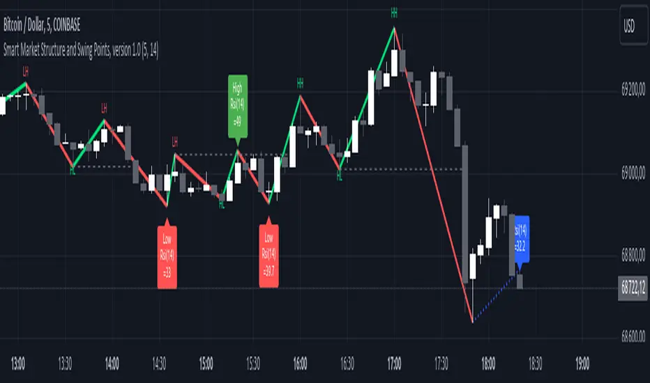
MOST on RSIMOST is applied on this RSI moving average with an extra default option added VAR/VIDYA (Variable Index Dynamic Moving Average)
MOST added on RSI has a Moving Average of RSI and a trailing percent stop level of the Moving Average that can be adjusted by changing the length of the MA and %percent of the stop level.
BUY SIGNAL when the Moving Average Line crosses above the MOST Line
LONG CONDITION when the Moving Average is above the MOST
SELL SIGNAL when Moving Average Line crosses below MOST Line
SHORT CONDITION when the Moving Average is below MOST
-MOST indicator advised to use with Variable Moving Average in the sideways market by its developer Anıl Özekşi, so there are a couple of alternative Moving Average OPTIONS to use in the calculation of MOST:
"SMA", "Bollinger Bands", "EMA", "SMMA (RMA)", "WMA", "VWMA", "VAR"
SMA: Simple Moving Average
EMA: Exponential Movin Average
SMMA (RMA: Smoothed Moving Average, Rolling/Running Moving Average
WMA: Weighted Moving Average
WWMA: Welles Wilder's Moving Average
VAR: Variable Index Dynamic Moving Average aka VIDYA
The Moving Average length and stop loss percent values must be increased for less reliable but late signals. Conversely, it must be decreased to have more and faster signals.
As this indicator is derived from TradingView's built-in RSI, it has Bollinger Bands bounding RSI and a tool that can be used for Bullish & Bearish divergences between the price and RSI. (Show Divergence option)
Finally, users may check the box "Show Signals" to visually see the BUY & SELL signals.
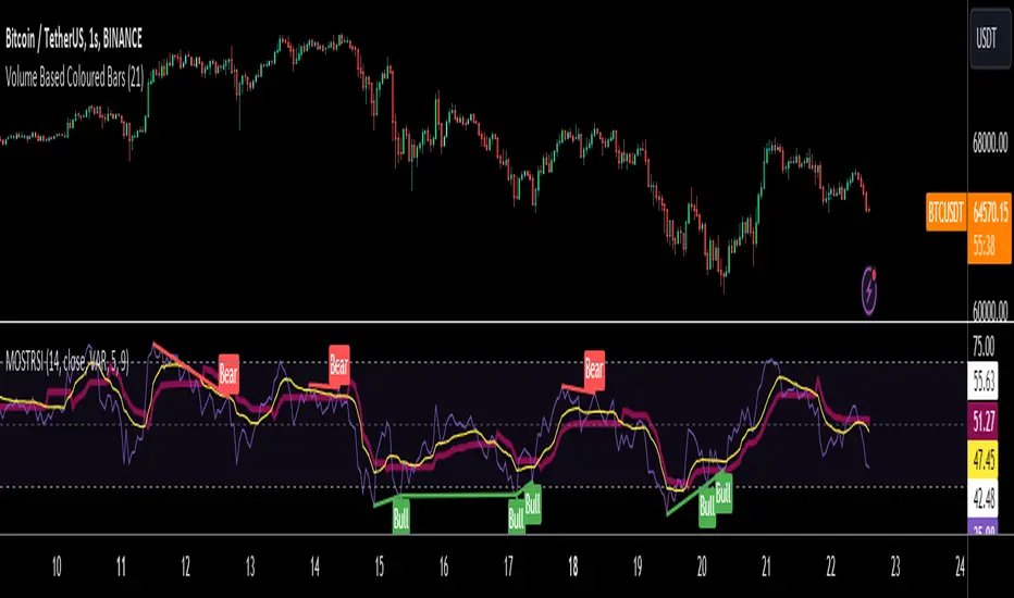
chrono_utilsLibrary "chrono_utils"
📝 Description
Collection of objects and common functions that are related to datetime windows session days and time ranges. The main purpose of this library is to handle time-related functionality and make it easy to reason about a future bar checking if it will be part of a predefined session and/or inside a datetime window. All existing session functionality I found in the documentation e.g. "not na(time(timeframe, session, timezone))" are not suitable for strategy scripts, since the execution of the orders is delayed by one bar, due to the script execution happening at the bar close. Moreover, a history operator with a negative value that looks forward is not allowed in any pinescript expression. So, a prediction for the next bar using the bars_back argument of "time()"" and "time_close()" was necessary. Thus, I created this library to overcome this small but very important limitation. In the meantime, I added useful functionality to handle session-based behavior. An interesting utility that emerged from this development is data anomaly detection where a comparison between the prediction and the actual value is happening. If those two values are different then a data inconsistency happens between the prediction bar and the actual bar (probably due to a holiday, half session day, a timezone change etc..)
🤔 How to Guide
To use the functionality this library provides in your script you have to import it first!
Copy the import statement of the latest release by pressing the copy button below and then paste it into your script. Give a short name to this library so you can refer to it later on. The import statement should look like this:
import jason5480/chrono_utils/2 as chr
To check if a future bar will be inside a window first of all you have to initialize a DateTimeWindow object.
A code example is the following:
var dateTimeWindow = chr.DateTimeWindow.new().init(fromDateTime = timestamp('01 Jan 2023 00:00'), toDateTime = timestamp('01 Jan 2024 00:00'))
Then you have to "ask" the dateTimeWindow if the future bar defined by an offset (default is 1 that corresponds th the next bar), will be inside that window:
// Filter bars outside of the datetime window
bool dateFilterApproval = dateTimeWindow.is_bar_included()
You can visualize the result by drawing the background of the bars that are outside the given window:
bgcolor(color = dateFilterApproval ? na : color.new(color.fuchsia, 90), offset = 1, title = 'Datetime Window Filter')
In the same way, you can "ask" the Session if the future bar defined by an offset it will be inside that session.
First of all, you should initialize a Session object.
A code example is the following:
var sess = chr.Session.new().from_sess_string(sess = '0800-1700:23456', refTimezone = 'UTC')
Then check if the given bar defined by the offset (default is 1 that corresponds th the next bar), will be inside the session like that:
// Filter bars outside the sessions
bool sessionFilterApproval = view.sess.is_bar_included()
You can visualize the result by drawing the background of the bars that are outside the given session:
bgcolor(color = sessionFilterApproval ? na : color.new(color.red, 90), offset = 1, title = 'Session Filter')
In case you want to visualize multiple session ranges you can create a SessionView object like that:
var view = SessionView.new().init(SessionDays.new().from_sess_string('2345'), array.from(SessionTimeRange.new().from_sess_string('0800-1600'), SessionTimeRange.new().from_sess_string('1300-2200')), array.from('London', 'New York'), array.from(color.blue, color.orange))
and then call the draw method of the SessionView object like that:
view.draw()
🏋️♂️ Please refer to the "EXAMPLE DATETIME WINDOW FILTER" and "EXAMPLE SESSION FILTER" regions of the script for more advanced code examples of how to utilize the full potential of this library, including user input settings and advanced visualization!
⚠️ Caveats
As I mentioned in the description there are some cases that the prediction of the next bar is not accurate. A wrong prediction will affect the outcome of the filtering. The main reasons this could happen are the following:
Public holidays when the market is closed
Half trading days usually before public holidays
Change in the daylight saving time (DST)
A data anomaly of the chart, where there are missing and/or inconsistent data.
A bug in this library (Please report by PM sending the symbol, timeframe, and settings)
Special thanks to @robbatt and @skinra for the constructive feedback 🏆. Without them, the exposed API of this library would be very lengthy and complicated to use. Thanks to them, now the user of this library will be able to get the most, with only a few lines of code!
