Trend Filter (2-pole) [BigBeluga]Trend Filter (2-pole)
The Trend Filter (2-pole) is an advanced trend-following indicator based on a two-pole filter, which smooths out market noise while effectively highlighting trends and their strength. It incorporates color gradients and support/resistance dots to enhance trend visualization and decision-making for traders.
SP500:
🔵What is a Two-Pole Filter?
A two-pole filter is a digital signal processing technique widely used in electronics, control systems, and time series data analysis to smooth data and reduce noise.
//@function Two-pole filter
//@param src (series float) Source data (e.g., price)
//@param length (float) Length of the filter (higher value means smoother output)
//@param damping (float) Damping factor for the filter
//@returns (series float) Filtered value
method two_pole_filter(float src, int length, float damping) =>
// Calculate filter coefficients
float omega = 2.0 * math.pi / length
float alpha = damping * omega
float beta = math.pow(omega, 2)
// Initialize the filter variables
var float f1 = na
var float f2 = na
// Update the filter
f1 := nz(f1 ) + alpha * (src - nz(f1 ))
f2 := nz(f2 ) + beta * (f1 - nz(f2 ))
f2
It operates using two cascaded smoothing stages (poles), allowing for a more refined and responsive output compared to simple moving averages or other basic filters.
Two-pole filters are particularly valued for their ability to maintain smooth transitions while reducing lag, making them ideal for applications where precision and responsiveness are critical.
In trading, this filter helps detect trends by smoothing price data while preserving significant directional changes.
🔵Key Features of the Indicator:
Gradient-Colored Trend Filter Line: The main filter line dynamically changes color based on trend strength and direction:
- Green: Strong uptrend.
- Red: Strong downtrend.
- Yellow: Indicates a transition phase, signaling potential trend shifts.
Support and Resistance Dots with Signals:
- Dots are plotted below the filter line during uptrends and above it during downtrends.
- These dots represent consecutive rising or falling conditions of the filter line, which traders can set in the settings (e.g., the number of consecutive rises or falls required).
- The dots often act as dynamic support or resistance levels, providing valuable guidance during trends.
- Trend Signals:
Customizable Sensitivity: The indicator allows traders to adjust the filter length, damping factor, and the threshold for rising/falling conditions, enabling it to adapt to different trading styles and timeframes.
Bar Color Option: The indicator can optionally color bars to match the gradient of the filter line, enhancing visual clarity of trends directly on the price chart.
🔵How It Works:
The Trend Filter (2-pole) smooths price data using a two-pole filter, which reduces noise and highlights the underlying trend.
The gradient coloring of the filter line helps traders visually assess the strength and direction of trends.
Rising and falling conditions of the filter line are tracked, and dots are plotted when consecutive conditions meet the threshold, acting as potential support or resistance levels during trends.
The yellow transition color signals periods of indecision, helping traders anticipate potential reversals or consolidations.
🔵Use Cases:
Identify and follow strong uptrends and downtrends with gradient-based visual cues.
Use the yellow transition color to anticipate trend shifts or consolidation zones.
Leverage the plotted dots as dynamic support and resistance levels to refine entry and exit strategies.
Combine with other indicators for confirmation of trends and reversals.
This indicator is perfect for traders who want a visually intuitive and highly customizable tool to spot trends, gauge their strength, and make informed trading decisions.
Поиск скриптов по запросу "VAR+计量模型+黄金期货"

MTF Countdown with Direction - AynetIndicator Definition and Inputs:
pineCopyindicator('MTF Countdown with Direction - Aynet', overlay = true)
This code creates a Multiple Time Frame (MTF) countdown indicator with direction
The overlay = true parameter places the indicator on top of the price chart
Timeframe Options:
Users can choose to show/hide the following timeframes:
1 minute
5 minutes
15 minutes
30 minutes
1 hour
4 hours
Daily
Time Calculations:
pineCopyget_current_time()
Calculates the current time
Converts Unix timestamp to seconds
Calculates time since midnight
Returns time broken down into hours, minutes, and seconds
Countdown Calculation:
pineCopyget_period_countdown(period_seconds)
Calculates remaining time for each timeframe
Computes elapsed time in current period
Returns remaining time in hours, minutes, and seconds
Direction and Closing Price Calculation:
Separate functions for each timeframe (get_direction_and_close_1m(), get_direction_and_close_5m(), etc.)
Each function:
Gets current closing price
Compares with previous closing price
Determines direction (up: 1, down: -1, sideways: 0)
Returns direction and closing price
Table Creation and Updates:
Creates a table in the top right corner
Table consists of 4 columns:
Period (Timeframe)
Time Left (Remaining time)
Direction (Shown with arrows)
Close (Closing price)
Each row has a different background color
Direction arrows:
Green up arrow (▲): Price rising
Red down arrow (▼): Price falling
Gray line (―): Price sideways
Dynamic Data Structures:
pineCopyvar timeframes = array.new_int()
var timeframe_names = array.new_string()
var show_array = array.new_bool()
Uses dynamic arrays for timeframes
Adds selected timeframes to arrays on first run
Key Features:
Shows remaining time until period close
Displays price direction for each timeframe
Shows current closing prices
All information in a single, easy-to-read table
This indicator helps traders by providing a comprehensive view of:
When each timeframe will close
The direction of price movement
Current closing prices
across multiple timeframes in a single table, making it easier to track market movements across different time periods.
The color-coding and arrow system makes it visually intuitive to understand market direction at a glance, while the countdown timer helps with timing decisions.

TrigWave Suite [InvestorUnknown]The TrigWave Suite combines Sine-weighted, Cosine-weighted, and Hyperbolic Tangent moving averages (HTMA) with a Directional Movement System (DMS) and a Relative Strength System (RSS).
Hyperbolic Tangent Moving Average (HTMA)
The HTMA smooths the price by applying a hyperbolic tangent transformation to the difference between the price and a simple moving average. It also adjusts this value by multiplying it by a standard deviation to create a more stable signal.
// Function to calculate Hyperbolic Tangent
tanh(x) =>
e_x = math.exp(x)
e_neg_x = math.exp(-x)
(e_x - e_neg_x) / (e_x + e_neg_x)
// Function to calculate Hyperbolic Tangent Moving Average
htma(src, len, mul) =>
tanh_src = tanh((src - ta.sma(src, len)) * mul) * ta.stdev(src, len) + ta.sma(src, len)
htma = ta.sma(tanh_src, len)
Sine-Weighted Moving Average (SWMA)
The SWMA applies sine-based weights to historical prices. This gives more weight to the central data points, making it responsive yet less prone to noise.
// Function to calculate the Sine-Weighted Moving Average
f_Sine_Weighted_MA(series float src, simple int length) =>
var float sine_weights = array.new_float(0)
array.clear(sine_weights) // Clear the array before recalculating weights
for i = 0 to length - 1
weight = math.sin((math.pi * (i + 1)) / length)
array.push(sine_weights, weight)
// Normalize the weights
sum_weights = array.sum(sine_weights)
for i = 0 to length - 1
norm_weight = array.get(sine_weights, i) / sum_weights
array.set(sine_weights, i, norm_weight)
// Calculate Sine-Weighted Moving Average
swma = 0.0
if bar_index >= length
for i = 0 to length - 1
swma := swma + array.get(sine_weights, i) * src
swma
Cosine-Weighted Moving Average (CWMA)
The CWMA uses cosine-based weights for data points, which produces a more stable trend-following behavior, especially in low-volatility markets.
f_Cosine_Weighted_MA(series float src, simple int length) =>
var float cosine_weights = array.new_float(0)
array.clear(cosine_weights) // Clear the array before recalculating weights
for i = 0 to length - 1
weight = math.cos((math.pi * (i + 1)) / length) + 1 // Shift by adding 1
array.push(cosine_weights, weight)
// Normalize the weights
sum_weights = array.sum(cosine_weights)
for i = 0 to length - 1
norm_weight = array.get(cosine_weights, i) / sum_weights
array.set(cosine_weights, i, norm_weight)
// Calculate Cosine-Weighted Moving Average
cwma = 0.0
if bar_index >= length
for i = 0 to length - 1
cwma := cwma + array.get(cosine_weights, i) * src
cwma
Directional Movement System (DMS)
DMS is used to identify trend direction and strength based on directional movement. It uses ADX to gauge trend strength and combines +DI and -DI for directional bias.
// Function to calculate Directional Movement System
f_DMS(simple int dmi_len, simple int adx_len) =>
up = ta.change(high)
down = -ta.change(low)
plusDM = na(up) ? na : (up > down and up > 0 ? up : 0)
minusDM = na(down) ? na : (down > up and down > 0 ? down : 0)
trur = ta.rma(ta.tr, dmi_len)
plus = fixnan(100 * ta.rma(plusDM, dmi_len) / trur)
minus = fixnan(100 * ta.rma(minusDM, dmi_len) / trur)
sum = plus + minus
adx = 100 * ta.rma(math.abs(plus - minus) / (sum == 0 ? 1 : sum), adx_len)
dms_up = plus > minus and adx > minus
dms_down = plus < minus and adx > plus
dms_neutral = not (dms_up or dms_down)
signal = dms_up ? 1 : dms_down ? -1 : 0
Relative Strength System (RSS)
RSS employs RSI and an adjustable moving average type (SMA, EMA, or HMA) to evaluate whether the market is in a bullish or bearish state.
// Function to calculate Relative Strength System
f_RSS(rsi_src, rsi_len, ma_type, ma_len) =>
rsi = ta.rsi(rsi_src, rsi_len)
ma = switch ma_type
"SMA" => ta.sma(rsi, ma_len)
"EMA" => ta.ema(rsi, ma_len)
"HMA" => ta.hma(rsi, ma_len)
signal = (rsi > ma and rsi > 50) ? 1 : (rsi < ma and rsi < 50) ? -1 : 0
ATR Adjustments
To minimize false signals, the HTMA, SWMA, and CWMA signals are adjusted with an Average True Range (ATR) filter:
// Calculate ATR adjusted components for HTMA, CWMA and SWMA
float atr = ta.atr(atr_len)
float htma_up = htma + (atr * atr_mult)
float htma_dn = htma - (atr * atr_mult)
float swma_up = swma + (atr * atr_mult)
float swma_dn = swma - (atr * atr_mult)
float cwma_up = cwma + (atr * atr_mult)
float cwma_dn = cwma - (atr * atr_mult)
This adjustment allows for better adaptation to varying market volatility, making the signal more reliable.
Signals and Trend Calculation
The indicator generates a Trend Signal by aggregating the output from each component. Each component provides a directional signal that is combined to form a unified trend reading. The trend value is then converted into a long (1), short (-1), or neutral (0) state.
Backtesting Mode and Performance Metrics
The Backtesting Mode includes a performance metrics table that compares the Buy and Hold strategy with the TrigWave Suite strategy. Key statistics like Sharpe Ratio, Sortino Ratio, and Omega Ratio are displayed to help users assess performance. Note that due to labels and plotchar use, automatic scaling may not function ideally in backtest mode.
Alerts and Visualization
Trend Direction Alerts: Set up alerts for long and short signals
Color Bars and Gradient Option: Bars are colored based on the trend direction, with an optional gradient for smoother visual feedback.
Important Notes
Customization: Default settings are experimental and not intended for trading/investing purposes. Users are encouraged to adjust and calibrate the settings to optimize results according to their trading style.
Backtest Results Disclaimer: Please note that backtest results are not indicative of future performance, and no strategy guarantees success.

FTMO Rules MonitorFTMO Rules Monitor: Stay on Track with Your FTMO Challenge Goals
TLDR; You can test with this template whether your strategy for one asset would pass the FTMO challenges step 1 then step 2, then with real money conditions.
Passing a prop firm challenge is ... challenging.
I believe a toolkit allowing to test in minutes whether a strategy would have passed a prop firm challenge in the past could be very powerful.
The FTMO Rules Monitor is designed to help you stay within FTMO’s strict risk management guidelines directly on your chart. Whether you’re aiming for the $10,000 or the $200,000 account challenge, this tool provides real-time tracking of your performance against FTMO’s rules to ensure you don’t accidentally breach any limits.
NOTES
The connected indicator for this post doesn't matter.
It's just a dummy double supertrends (see below)
The strategy results for this script post does not matter as I'm posting a FTMO rules template on which you can connect any indicator/strategy.
//@version=5
indicator("Supertrends", overlay=true)
// Supertrend 1 Parameters
var string ST1 = "Supertrend 1 Settings"
st1_atrPeriod = input.int(10, "ATR Period", minval=1, maxval=50, group=ST1)
st1_factor = input.float(2, "Factor", minval=0.5, maxval=10, step=0.5, group=ST1)
// Supertrend 2 Parameters
var string ST2 = "Supertrend 2 Settings"
st2_atrPeriod = input.int(14, "ATR Period", minval=1, maxval=50, group=ST2)
st2_factor = input.float(3, "Factor", minval=0.5, maxval=10, step=0.5, group=ST2)
// Calculate Supertrends
= ta.supertrend(st1_factor, st1_atrPeriod)
= ta.supertrend(st2_factor, st2_atrPeriod)
// Entry conditions
longCondition = direction1 == -1 and direction2 == -1 and direction1 == 1
shortCondition = direction1 == 1 and direction2 == 1 and direction1 == -1
// Optional: Plot Supertrends
plot(supertrend1, "Supertrend 1", color = direction1 == -1 ? color.green : color.red, linewidth=3)
plot(supertrend2, "Supertrend 2", color = direction2 == -1 ? color.lime : color.maroon, linewidth=3)
plotshape(series=longCondition, location=location.belowbar, color=color.green, style=shape.triangleup, title="Long")
plotshape(series=shortCondition, location=location.abovebar, color=color.red, style=shape.triangledown, title="Short")
signal = longCondition ? 1 : shortCondition ? -1 : na
plot(signal, "Signal", display = display.data_window)
To connect your indicator to this FTMO rules monitor template, please update it as follow
Create a signal variable to store 1 for the long/buy signal or -1 for the short/sell signal
Plot it in the display.data_window panel so that it doesn't clutter your chart
signal = longCondition ? 1 : shortCondition ? -1 : na
plot(signal, "Signal", display = display.data_window)
In the FTMO Rules Monitor template, I'm capturing this external signal with this input.source variable
entry_connector = input.source(close, "Entry Connector", group="Entry Connector")
longCondition = entry_connector == 1
shortCondition = entry_connector == -1
🔶 USAGE
This indicator displays essential FTMO Challenge rules and tracks your progress toward meeting each one. Here’s what’s monitored:
Max Daily Loss
• 10k Account: $500
• 25k Account: $1,250
• 50k Account: $2,500
• 100k Account: $5,000
• 200k Account: $10,000
Max Total Loss
• 10k Account: $1,000
• 25k Account: $2,500
• 50k Account: $5,000
• 100k Account: $10,000
• 200k Account: $20,000
Profit Target
• 10k Account: $1,000
• 25k Account: $2,500
• 50k Account: $5,000
• 100k Account: $10,000
• 200k Account: $20,000
Minimum Trading Days: 4 consecutive days for all account sizes
🔹 Key Features
1. Real-Time Compliance Check
The FTMO Rules Monitor keeps track of your daily and total losses, profit targets, and trading days. Each metric updates in real-time, giving you peace of mind that you’re within FTMO’s rules.
2. Color-Coded Visual Feedback
Each rule’s status is shown clearly with a ✓ for compliance or ✗ if the limit is breached. When a rule is broken, the indicator highlights it in red, so there’s no confusion.
3. Completion Notification
Once all FTMO requirements are met, the indicator closes all open positions and displays a celebratory message on your chart, letting you know you’ve successfully completed the challenge.
4. Easy-to-Read Table
A table on your chart provides an overview of each rule, your target, current performance, and whether you’re meeting each goal. The table adjusts its color scheme based on your chart settings for optimal visibility.
5. Dynamic Position Sizing
Integrated ATR-based position sizing helps you manage risk and avoid large drawdowns, ensuring each trade aligns with FTMO’s risk management principles.
Daveatt

Prometheus Fractal WaveThe Fractal Wave is an indicator that uses a fractal analysis to determine where reversals may happen. This is done through a Fractal process, making sure a price point is in a certain set and then getting a Distance metric.
Calculation:
A bullish Fractal is defined by the current bar’s high being less than the last bar’s high, and the last bar’s high being greater than the second to last bar’s high, and the last bar’s high being greater than the third to last bar’s high.
A bearish Fractal is defined by the current low being greater than the last bar’s low, and the last bar’s low being less than the second to last bar’s low, and the last bar’s low being less than the third to last bar’s low.
When there is that bullish or bearish fractal the value we store is either the last bar’s high or low respective to bullish or bearish fractal.
Once we have that value stored we either subtract the last bar’s low from the bullish Fractal value, and subtract the last bar’s high from the bearish Fractal value. Those are our Distances.
Code:
isBullishFractal() =>
high > high and high < high and high > high
isBearishFractal() =>
low < low and low > low and low < low
var float lastBullishFractal = na
var float lastBearishFractal = na
if isBullishFractal() and barstate.isconfirmed
lastBullishFractal := high
if isBearishFractal() and barstate.isconfirmed
lastBearishFractal := low
//------------------------------
//-------CACLULATION------------
//------------------------------
bullWaveDistance = na(lastBullishFractal) ? na : lastBullishFractal - low
bearWaveDistance = na(lastBearishFractal) ? na : high - lastBearishFractal
We then plot the bullish distance and the negative bearish distance.
The trade scenarios come from when one breaks the zero line and then goes back above or below. So if the last bullish distance was below 0 and is now above, or if the last negative bearish distance was above 0 and now below. We plot a green label below a candle for a bullish scenario, or a red label above a candle for a bearish one, you can turn them on or off.
Code:
plot(bullWaveDistance, color=color.green, title="Bull Wave Distance", linewidth=2)
plot(-bearWaveDistance, color=color.red, title="Bear Wave Distance", linewidth=2)
plot(0, "Zero Line", color=color.gray, display = display.pane)
bearish_reversal = plot_labels ? bullWaveDistance < 0 and bullWaveDistance > 0 : na
bullish_reversal = plot_labels ? -bearWaveDistance > 0 and -bearWaveDistance < 0 : na
plotshape(bullish_reversal, location=location.belowbar, color=color.green, style=shape.labelup, title="Bullish Fractal", text="↑", display = display.all - display.status_line, force_overlay = true)
plotshape(bearish_reversal, location=location.abovebar, color=color.red, style=shape.labeldown, title="Bearish Fractal", text="↓", display = display.all - display.status_line, force_overlay = true)
We can see in this daily NASDAQ:QQQ chart that the indicator gives us marks that can either be used as Reversal signals or as breathers in the trend.
Since it is designed to provide reversals, on something like Gold where the uptrend has been strong, the signals may be just short breathers, not full blown strong reversal signs.
The indicator works just as well intra day as it does on larger timeframes.
We encourage traders to not follow indicators blindly, none are 100% accurate. Please comment on any desired updates, all criticism is welcome!

PRINT_TYPELibrary "PRINT_TYPE"
Inputs
Inputs objects
Fields:
inbalance_percent (series int) : percentage coefficient to determine the Imbalance of price levels
stacked_input (series int) : minimum number of consecutive Imbalance levels required to draw extended lines
show_summary_footprint (series bool)
procent_volume_area (series int) : definition size Value area
new_imbalance_cond (series bool) : bool input for setup alert on new imbalance buy and sell
new_imbalance_line_cond (series bool) : bool input for setup alert on new imbalance line buy and sell
stop_past_imbalance_line_cond (series bool) : bool input for setup alert on stop past imbalance line buy and sell
Constants
Constants all Constants objects
Fields:
imbalance_high_char (series string) : char for printing buy imbalance
imbalance_low_char (series string) : char for printing sell imbalance
color_title_sell (series color) : color for footprint sell
color_title_buy (series color) : color for footprint buy
color_line_sell (series color) : color for sell line
color_line_buy (series color) : color for buy line
color_title_none (series color) : color None
Calculation_data
Calculation_data data for calculating
Fields:
detail_open (array) : array open from calculation timeframe
detail_high (array) : array high from calculation timeframe
detail_low (array) : array low from calculation timeframe
detail_close (array) : array close from calculation timeframe
detail_vol (array) : array volume from calculation timeframe
previos_detail_close (array) : array close from calculation timeframe
isBuyVolume (series bool) : attribute previosly bar buy or sell
Footprint_row
Footprint_row objects one footprint row
Fields:
price (series float) : row price
buy_vol (series float) : buy volume
sell_vol (series float) : sell volume
imbalance_buy (series bool) : attribute buy inbalance
imbalance_sell (series bool) : attribute sell imbalance
buy_vol_box (series box) : for ptinting buy volume
sell_vol_box (series box) : for printing sell volume
buy_vp_box (series box) : for ptinting volume profile buy
sell_vp_box (series box) : for ptinting volume profile sell
row_line (series label) : for ptinting row price
empty (series bool) : = true attribute row with zero volume buy and zero volume sell
Imbalance_line_var_object
Imbalance_line_var_object var objects printing and calculation imbalance line
Fields:
cum_buy_line (array) : line array for saving all history buy imbalance line
cum_sell_line (array) : line array for saving all history sell imbalance line
Imbalance_line
Imbalance_line objects printing and calculation imbalance line
Fields:
buy_price_line (array) : float array for saving buy imbalance price level
sell_price_line (array) : float array for saving sell imbalance price level
var_imba_line (Imbalance_line_var_object) : var objects this type
Footprint_bar
Footprint_bar all objects one bar with footprint
Fields:
foot_rows (array) : objects one row footprint
imba_line (Imbalance_line) : objects imbalance line
row_size (series float) : size rows
total_vol (series float) : total volume one footprint bar
foot_buy_vol (series float) : buy volume one footprint bar
foot_sell_vol (series float) : sell volume one footprint bar
foot_max_price_vol (map) : map with one value - price row with max volume buy + sell
calc_data (Calculation_data) : objects with detail data from calculation resolution
Support_objects
Support_objects support object for footprint calculation
Fields:
consts (Constants) : all consts objects
inp (Inputs) : all input objects
bar_index_show_condition (series bool) : calculation bool value for show all objects footprint
row_line_color (series color) : calculation value - color for row price
dop_info (series string)
show_table_cond (series bool)
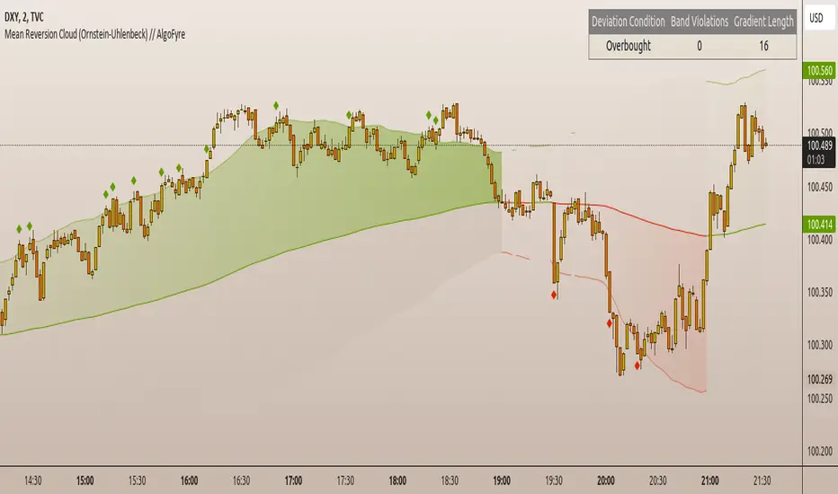
Mean Reversion Cloud (Ornstein-Uhlenbeck) // AlgoFyreThe Mean Reversion Cloud (Ornstein-Uhlenbeck) indicator detects mean-reversion opportunities by applying the Ornstein-Uhlenbeck process. It calculates a dynamic mean using an Exponential Weighted Moving Average, surrounded by volatility bands, signaling potential buy/sell points when prices deviate.
TABLE OF CONTENTS
🔶 ORIGINALITY
🔸Adaptive Mean Calculation
🔸Volatility-Based Cloud
🔸Speed of Reversion (θ)
🔶 FUNCTIONALITY
🔸Dynamic Mean and Volatility Bands
🞘 How it works
🞘 How to calculate
🞘 Code extract
🔸Visualization via Table and Plotshapes
🞘 Table Overview
🞘 Plotshapes Explanation
🞘 Code extract
🔶 INSTRUCTIONS
🔸Step-by-Step Guidelines
🞘 Setting Up the Indicator
🞘 Understanding What to Look For on the Chart
🞘 Possible Entry Signals
🞘 Possible Take Profit Strategies
🞘 Possible Stop-Loss Levels
🞘 Additional Tips
🔸Customize settings
🔶 CONCLUSION
▅▅▅▅▅▅▅▅▅▅▅▅▅▅▅▅▅▅▅▅▅▅▅▅▅▅▅▅▅▅▅▅▅▅▅▅▅▅▅▅▅▅▅▅▅▅
🔶 ORIGINALITY The Mean Reversion Cloud (Ornstein-Uhlenbeck) is a unique indicator that applies the Ornstein-Uhlenbeck stochastic process to identify mean-reverting behavior in asset prices. Unlike traditional moving average-based indicators, this model uses an Exponentially Weighted Moving Average (EWMA) to calculate the long-term mean, dynamically adjusting to recent price movements while still considering all historical data. It also incorporates volatility bands, providing a "cloud" that visually highlights overbought or oversold conditions. By calculating the speed of mean reversion (θ) through the autocorrelation of log returns, this indicator offers traders a more nuanced and mathematically robust tool for identifying mean-reversion opportunities. These innovations make it especially useful for markets that exhibit range-bound characteristics, offering timely buy and sell signals based on statistical deviations from the mean.
🔸Adaptive Mean Calculation Traditional MA indicators use fixed lengths, which can lead to lagging signals or over-sensitivity in volatile markets. The Mean Reversion Cloud uses an Exponentially Weighted Moving Average (EWMA), which adapts to price movements by dynamically adjusting its calculation, offering a more responsive mean.
🔸Volatility-Based Cloud Unlike simple moving averages that only plot a single line, the Mean Reversion Cloud surrounds the dynamic mean with volatility bands. These bands, based on standard deviations, provide traders with a visual cue of when prices are statistically likely to revert, highlighting potential reversal zones.
🔸Speed of Reversion (θ) The indicator goes beyond price averages by calculating the speed at which the price reverts to the mean (θ), using the autocorrelation of log returns. This gives traders an additional tool for estimating the likelihood and timing of mean reversion, making the signals more reliable in practice.
🔶 FUNCTIONALITY The Mean Reversion Cloud (Ornstein-Uhlenbeck) indicator is designed to detect potential mean-reversion opportunities in asset prices by applying the Ornstein-Uhlenbeck stochastic process. It calculates a dynamic mean through the Exponentially Weighted Moving Average (EWMA) and plots volatility bands based on the standard deviation of the asset's price over a specified period. These bands create a "cloud" that represents expected price fluctuations, helping traders to identify overbought or oversold conditions. By calculating the speed of reversion (θ) from the autocorrelation of log returns, the indicator offers a more refined way of assessing how quickly prices may revert to the mean. Additionally, the inclusion of volatility provides a comprehensive view of market conditions, allowing for more accurate buy and sell signals.
Let's dive into the details:
🔸Dynamic Mean and Volatility Bands The dynamic mean (μ) is calculated using the EWMA, giving more weight to recent prices but considering all historical data. This process closely resembles the Ornstein-Uhlenbeck (OU) process, which models the tendency of a stochastic variable (such as price) to revert to its mean over time. Volatility bands are plotted around the mean using standard deviation, forming the "cloud" that signals overbought or oversold conditions. The cloud adapts dynamically to price fluctuations and market volatility, making it a versatile tool for mean-reversion strategies. 🞘 How it works Step one: Calculate the dynamic mean (μ) The Ornstein-Uhlenbeck process describes how a variable, such as an asset's price, tends to revert to a long-term mean while subject to random fluctuations. In this indicator, the EWMA is used to compute the dynamic mean (μ), mimicking the mean-reverting behavior of the OU process. Use the EWMA formula to compute a weighted mean that adjusts to recent price movements. Assign exponentially decreasing weights to older data while giving more emphasis to current prices. Step two: Plot volatility bands Calculate the standard deviation of the price over a user-defined period to determine market volatility. Position the upper and lower bands around the mean by adding and subtracting a multiple of the standard deviation. 🞘 How to calculate Exponential Weighted Moving Average (EWMA)
The EWMA dynamically adjusts to recent price movements:
mu_t = lambda * mu_{t-1} + (1 - lambda) * P_t
Where mu_t is the mean at time t, lambda is the decay factor, and P_t is the price at time t. The higher the decay factor, the more weight is given to recent data.
Autocorrelation (ρ) and Standard Deviation (σ)
To measure mean reversion speed and volatility: rho = correlation(log(close), log(close ), length) Where rho is the autocorrelation of log returns over a specified period.
To calculate volatility:
sigma = stdev(close, length)
Where sigma is the standard deviation of the asset's closing price over a specified length.
Upper and Lower Bands
The upper and lower bands are calculated as follows:
upper_band = mu + (threshold * sigma)
lower_band = mu - (threshold * sigma)
Where threshold is a multiplier for the standard deviation, usually set to 2. These bands represent the range within which the price is expected to fluctuate, based on current volatility and the mean.
🞘 Code extract // Calculate Returns
returns = math.log(close / close )
// Calculate Long-Term Mean (μ) using EWMA over the entire dataset
var float ewma_mu = na // Initialize ewma_mu as 'na'
ewma_mu := na(ewma_mu ) ? close : decay_factor * ewma_mu + (1 - decay_factor) * close
mu = ewma_mu
// Calculate Autocorrelation at Lag 1
rho1 = ta.correlation(returns, returns , corr_length)
// Ensure rho1 is within valid range to avoid errors
rho1 := na(rho1) or rho1 <= 0 ? 0.0001 : rho1
// Calculate Speed of Mean Reversion (θ)
theta = -math.log(rho1)
// Calculate Volatility (σ)
sigma = ta.stdev(close, corr_length)
// Calculate Upper and Lower Bands
upper_band = mu + threshold * sigma
lower_band = mu - threshold * sigma
🔸Visualization via Table and Plotshapes
The table shows key statistics such as the current value of the dynamic mean (μ), the number of times the price has crossed the upper or lower bands, and the consecutive number of bars that the price has remained in an overbought or oversold state.
Plotshapes (diamonds) are used to signal buy and sell opportunities. A green diamond below the price suggests a buy signal when the price crosses below the lower band, and a red diamond above the price indicates a sell signal when the price crosses above the upper band.
The table and plotshapes provide a comprehensive visualization, combining both statistical and actionable information to aid decision-making.
🞘 Code extract // Reset consecutive_bars when price crosses the mean
var consecutive_bars = 0
if (close < mu and close >= mu) or (close > mu and close <= mu)
consecutive_bars := 0
else if math.abs(deviation) > 0
consecutive_bars := math.min(consecutive_bars + 1, dev_length)
transparency = math.max(0, math.min(100, 100 - (consecutive_bars * 100 / dev_length)))
🔶 INSTRUCTIONS
The Mean Reversion Cloud (Ornstein-Uhlenbeck) indicator can be set up by adding it to your TradingView chart and configuring parameters such as the decay factor, autocorrelation length, and volatility threshold to suit current market conditions. Look for price crossovers and deviations from the calculated mean for potential entry signals. Use the upper and lower bands as dynamic support/resistance levels for setting take profit and stop-loss orders. Combining this indicator with additional trend-following or momentum-based indicators can improve signal accuracy. Adjust settings for better mean-reversion detection and risk management.
🔸Step-by-Step Guidelines
🞘 Setting Up the Indicator
Adding the Indicator to the Chart:
Go to your TradingView chart.
Click on the "Indicators" button at the top.
Search for "Mean Reversion Cloud (Ornstein-Uhlenbeck)" in the indicators list.
Click on the indicator to add it to your chart.
Configuring the Indicator:
Open the indicator settings by clicking on the gear icon next to its name on the chart.
Decay Factor: Adjust the decay factor (λ) to control the responsiveness of the mean calculation. A higher value prioritizes recent data.
Autocorrelation Length: Set the autocorrelation length (θ) for calculating the speed of mean reversion. Longer lengths consider more historical data.
Threshold: Define the number of standard deviations for the upper and lower bands to determine how far price must deviate to trigger a signal.
Chart Setup:
Select the appropriate timeframe (e.g., 1-hour, daily) based on your trading strategy.
Consider using other indicators such as RSI or MACD to confirm buy and sell signals.
🞘 Understanding What to Look For on the Chart
Indicator Behavior:
Observe how the price interacts with the dynamic mean and volatility bands. The price staying within the bands suggests mean-reverting behavior, while crossing the bands signals potential entry points.
The indicator calculates overbought/oversold conditions based on deviation from the mean, highlighted by color-coded cloud areas on the chart.
Crossovers and Deviation:
Look for crossovers between the price and the mean (μ) or the bands. A bullish crossover occurs when the price crosses below the lower band, signaling a potential buying opportunity.
A bearish crossover occurs when the price crosses above the upper band, suggesting a potential sell signal.
Deviations from the mean indicate market extremes. A large deviation indicates that the price is far from the mean, suggesting a potential reversal.
Slope and Direction:
Pay attention to the slope of the mean (μ). A rising slope suggests bullish market conditions, while a declining slope signals a bearish market.
The steepness of the slope can indicate the strength of the mean-reversion trend.
🞘 Possible Entry Signals
Bullish Entry:
Crossover Entry: Enter a long position when the price crosses below the lower band with a positive deviation from the mean.
Confirmation Entry: Use additional indicators like RSI (above 50) or increasing volume to confirm the bullish signal.
Bearish Entry:
Crossover Entry: Enter a short position when the price crosses above the upper band with a negative deviation from the mean.
Confirmation Entry: Look for RSI (below 50) or decreasing volume to confirm the bearish signal.
Deviation Confirmation:
Enter trades when the deviation from the mean is significant, indicating that the price has strayed far from its expected value and is likely to revert.
🞘 Possible Take Profit Strategies
Static Take Profit Levels:
Set predefined take profit levels based on historical volatility, using the upper and lower bands as guides.
Place take profit orders near recent support/resistance levels, ensuring you're capitalizing on the mean-reversion behavior.
Trailing Stop Loss:
Use a trailing stop based on a percentage of the price deviation from the mean to lock in profits as the trend progresses.
Adjust the trailing stop dynamically along the calculated bands to protect profits as the price returns to the mean.
Deviation-Based Exits:
Exit when the deviation from the mean starts to decrease, signaling that the price is returning to its equilibrium.
🞘 Possible Stop-Loss Levels
Initial Stop Loss:
Place an initial stop loss outside the lower band (for long positions) or above the upper band (for short positions) to protect against excessive deviations.
Use a volatility-based buffer to avoid getting stopped out during normal price fluctuations.
Dynamic Stop Loss:
Move the stop loss closer to the mean as the price converges back towards equilibrium, reducing risk.
Adjust the stop loss dynamically along the bands to account for sudden market movements.
🞘 Additional Tips
Combine with Other Indicators:
Enhance your strategy by combining the Mean Reversion Cloud with momentum indicators like MACD, RSI, or Bollinger Bands to confirm market conditions.
Backtesting and Practice:
Backtest the indicator on historical data to understand how it performs in various market environments.
Practice using the indicator on a demo account before implementing it in live trading.
Market Awareness:
Keep an eye on market news and events that might cause extreme price movements. The indicator reacts to price data and might not account for news-driven events that can cause large deviations.
🔸Customize settings 🞘 Decay Factor (λ): Defines the weight assigned to recent price data in the calculation of the mean. A value closer to 1 places more emphasis on recent prices, while lower values create a smoother, more lagging mean.
🞘 Autocorrelation Length (θ): Sets the period for calculating the speed of mean reversion and volatility. Longer lengths capture more historical data, providing smoother calculations, while shorter lengths make the indicator more responsive.
🞘 Threshold (σ): Specifies the number of standard deviations used to create the upper and lower bands. Higher thresholds widen the bands, producing fewer signals, while lower thresholds tighten the bands for more frequent signals.
🞘 Max Gradient Length (γ): Determines the maximum number of consecutive bars for calculating the deviation gradient. This setting impacts the transparency of the plotted bands based on the length of deviation from the mean.
🔶 CONCLUSION
The Mean Reversion Cloud (Ornstein-Uhlenbeck) indicator offers a sophisticated approach to identifying mean-reversion opportunities by applying the Ornstein-Uhlenbeck stochastic process. This dynamic indicator calculates a responsive mean using an Exponentially Weighted Moving Average (EWMA) and plots volatility-based bands to highlight overbought and oversold conditions. By incorporating advanced statistical measures like autocorrelation and standard deviation, traders can better assess market extremes and potential reversals. The indicator’s ability to adapt to price behavior makes it a versatile tool for traders focused on both short-term price deviations and longer-term mean-reversion strategies. With its unique blend of statistical rigor and visual clarity, the Mean Reversion Cloud provides an invaluable tool for understanding and capitalizing on market inefficiencies.
Realized Price Oscillator [InvestorUnknown]Overview
The Realized Price Oscillator is a fundamental analysis tool designed to assess Bitcoin's price dynamics relative to its realized price. The indicator calculates various metrics using data from the realized market capitalization and total supply. It applies normalization techniques to scale values within a specified range, helping investors identify overbought or oversold conditions over the long time horizon. The oscillator also features DCA-based signals to assist in strategic market entry and exit.
Key Features
1. Normalization and Scaling:
The indicator scales values using a limit that can be adjusted for decimal precision (Limit). It allows for both positive and negative values, providing flexibility in analysis.
Decay functionality is included to progressively reduce the extreme values over time, ensuring recent data impacts the oscillator more than older data.
f_rescale(float value, float min, float max, float limit, bool negatives) =>
((limit * (negatives ? 2 : 1)) * (value - min) / (max - min)) - (negatives ? limit : 0)
2. Realized Price Oscillator Calculation:
Realized Price Oscillator is computed using logarithmic differences between the open, high, low, and close prices and the realized price. This helps in identifying how the current market price compares with the average cost basis of the Bitcoin supply.
f_realized_price_oscillator(float realized_price) =>
rpo_o = math.log(open / realized_price)
rpo_h = math.log(high / realized_price)
rpo_l = math.log(low / realized_price)
rpo_c = math.log(close / realized_price)
3. Oscillator Normalization:
The normalized oscillator calculates the range between the maximum and minimum values over time. It adjusts the oscillator values based on these bounds, considering a decay factor. This normalized range assists in consistent signal generation.
normalized_oscillator(float x, float b) =>
float oscillator = b
var float min = na
var float max = na
if (oscillator > max or na(max)) and time >= normalization_start_date
max := oscillator
if (min > oscillator or na(min)) and time >= normalization_start_date
min := oscillator
if time >= normalization_start_date
max := max * decay
min := min * decay
normalized_oscillator = f_rescale(x, min, max, lim, neg)
4. Dollar-Cost Averaging (DCA) Signals:
DCA-based signals are generated using user-defined thresholds (DCA IN and DCA OUT). The oscillator triggers buy signals when the normalized low value falls below the DCA IN threshold and sell signals when the normalized high value exceeds the DCA OUT threshold.
5. Visual Representation:
The indicator plots candlestick representations of the normalized Realized Price Oscillator values (open, high, low, close) over time, starting from a specified date (plot_start_date).
Colors are dynamically adjusted using a gradient to represent the state of the oscillator, ranging from green (buy zone) to red (sell zone). Background and bar colors also change based on DCA conditions.
How It Works
Data Sourcing: Realized price data is sourced using Bitcoin’s realized market cap (BTC_MARKETCAPREAL) and total supply (BTC_SUPPLY).
Realized Price Oscillator Metrics: Logarithmic differences between price and realized price are computed to generate Realized Price Oscillator values for open, high, low, and close.
Normalization: The indicator rescales the oscillator values based on a defined limit, adjusting for negative values if allowed. It employs a decay factor to reduce the influence of historical extremes.
Conclusion
The Realized Price Oscillator is a sophisticated tool that combines market price analysis with realized price metrics to offer a robust framework for understanding Bitcoin's valuation. By leveraging normalization techniques and DCA thresholds, it provides actionable insights for long-term investing strategies.

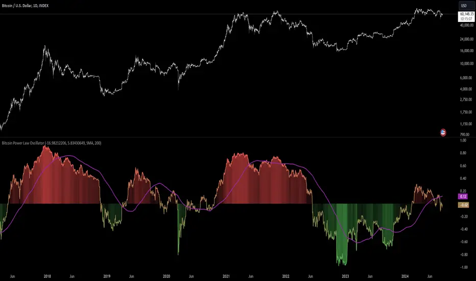
Bitcoin Power Law Oscillator [InvestorUnknown]The Bitcoin Power Law Oscillator is a specialized tool designed for long-term mean-reversion analysis of Bitcoin's price relative to a theoretical midline derived from the Bitcoin Power Law model (made by capriole_charles). This oscillator helps investors identify whether Bitcoin is currently overbought, oversold, or near its fair value according to this mathematical model.
Key Features:
Power Law Model Integration: The oscillator is based on the midline of the Bitcoin Power Law, which is calculated using regression coefficients (A and B) applied to the logarithm of the number of days since Bitcoin’s inception. This midline represents a theoretical fair value for Bitcoin over time.
Midline Distance Calculation: The distance between Bitcoin’s current price and the Power Law midline is computed as a percentage, indicating how far above or below the price is from this theoretical value.
float a = input.float (-16.98212206, 'Regression Coef. A', group = "Power Law Settings")
float b = input.float (5.83430649, 'Regression Coef. B', group = "Power Law Settings")
normalization_start_date = timestamp(2011,1,1)
calculation_start_date = time == timestamp(2010, 7, 19, 0, 0) // First BLX Bitcoin Date
int days_since = request.security('BNC:BLX', 'D', ta.barssince(calculation_start_date))
bar() =>
= request.security('BNC:BLX', 'D', bar())
int offset = 564 // days between 2009/1/1 and "calculation_start_date"
int days = days_since + offset
float e = a + b * math.log10(days)
float y = math.pow(10, e)
float midline_distance = math.round((y / btc_close - 1.0) * 100)
Oscillator Normalization: The raw distance is converted into a normalized oscillator, which fluctuates between -1 and 1. This normalization adjusts the oscillator to account for historical extremes, making it easier to compare current conditions with past market behavior.
float oscillator = -midline_distance
var float min = na
var float max = na
if (oscillator > max or na(max)) and time >= normalization_start_date
max := oscillator
if (min > oscillator or na(min)) and time >= normalization_start_date
min := oscillator
rescale(float value, float min, float max) =>
(2 * (value - min) / (max - min)) - 1
normalized_oscillator = rescale(oscillator, min, max)
Overbought/Oversold Identification: The oscillator provides a clear visual representation, where values near 1 suggest Bitcoin is overbought, and values near -1 indicate it is oversold. This can help identify potential reversal points or areas of significant market imbalance.
Optional Moving Average: Users can overlay a moving average (either SMA or EMA) on the oscillator to smooth out short-term fluctuations and focus on longer-term trends. This is particularly useful for confirming trend reversals or persistent overbought/oversold conditions.
This indicator is particularly useful for long-term Bitcoin investors who wish to gauge the market's mean-reversion tendencies based on a well-established theoretical model. By focusing on the Power Law’s midline, users can gain insights into whether Bitcoin’s current price deviates significantly from what historical trends would suggest as a fair value.
Adaptive Trend Classification: Moving Averages [InvestorUnknown]Adaptive Trend Classification: Moving Averages
Overview
The Adaptive Trend Classification (ATC) Moving Averages indicator is a robust and adaptable investing tool designed to provide dynamic signals based on various types of moving averages and their lengths. This indicator incorporates multiple layers of adaptability to enhance its effectiveness in various market conditions.
Key Features
Adaptability of Moving Average Types and Lengths: The indicator utilizes different types of moving averages (EMA, HMA, WMA, DEMA, LSMA, KAMA) with customizable lengths to adjust to market conditions.
Dynamic Weighting Based on Performance: ] Weights are assigned to each moving average based on the equity they generate, with considerations for a cutout period and decay rate to manage (reduce) the influence of past performances.
Exponential Growth Adjustment: The influence of recent performance is enhanced through an adjustable exponential growth factor, ensuring that more recent data has a greater impact on the signal.
Calibration Mode: Allows users to fine-tune the indicator settings for specific signal periods and backtesting, ensuring optimized performance.
Visualization Options: Multiple customization options for plotting moving averages, color bars, and signal arrows, enhancing the clarity of the visual output.
Alerts: Configurable alert settings to notify users based on specific moving average crossovers or the average signal.
User Inputs
Adaptability Settings
λ (Lambda): Specifies the growth rate for exponential growth calculations.
Decay (%): Determines the rate of depreciation applied to the equity over time.
CutOut Period: Sets the period after which equity calculations start, allowing for a focus on specific time ranges.
Robustness Lengths: Defines the range of robustness for equity calculation with options for Narrow, Medium, or Wide adjustments.
Long/Short Threshold: Sets thresholds for long and short signals.
Calculation Source: The data source used for calculations (e.g., close price).
Moving Averages Settings
Lengths and Weights: Allows customization of lengths and initial weights for each moving average type (EMA, HMA, WMA, DEMA, LSMA, KAMA).
Calibration Mode
Calibration Mode: Enables calibration for fine-tuning inputs.
Calibrate: Specifies which moving average type to calibrate.
Strategy View: Shifts entries and exits by one bar for non-repainting backtesting.
Calculation Logic
Rate of Change (R): Calculates the rate of change in the price.
Set of Moving Averages: Generates multiple moving averages with different lengths for each type.
diflen(length) =>
int L1 = na, int L_1 = na
int L2 = na, int L_2 = na
int L3 = na, int L_3 = na
int L4 = na, int L_4 = na
if robustness == "Narrow"
L1 := length + 1, L_1 := length - 1
L2 := length + 2, L_2 := length - 2
L3 := length + 3, L_3 := length - 3
L4 := length + 4, L_4 := length - 4
else if robustness == "Medium"
L1 := length + 1, L_1 := length - 1
L2 := length + 2, L_2 := length - 2
L3 := length + 4, L_3 := length - 4
L4 := length + 6, L_4 := length - 6
else
L1 := length + 1, L_1 := length - 1
L2 := length + 3, L_2 := length - 3
L3 := length + 5, L_3 := length - 5
L4 := length + 7, L_4 := length - 7
// Function to calculate different types of moving averages
ma_calculation(source, length, ma_type) =>
if ma_type == "EMA"
ta.ema(source, length)
else if ma_type == "HMA"
ta.sma(source, length)
else if ma_type == "WMA"
ta.wma(source, length)
else if ma_type == "DEMA"
ta.dema(source, length)
else if ma_type == "LSMA"
lsma(source,length)
else if ma_type == "KAMA"
kama(source, length)
else
na
// Function to create a set of moving averages with different lengths
SetOfMovingAverages(length, source, ma_type) =>
= diflen(length)
MA = ma_calculation(source, length, ma_type)
MA1 = ma_calculation(source, L1, ma_type)
MA2 = ma_calculation(source, L2, ma_type)
MA3 = ma_calculation(source, L3, ma_type)
MA4 = ma_calculation(source, L4, ma_type)
MA_1 = ma_calculation(source, L_1, ma_type)
MA_2 = ma_calculation(source, L_2, ma_type)
MA_3 = ma_calculation(source, L_3, ma_type)
MA_4 = ma_calculation(source, L_4, ma_type)
Exponential Growth Factor: Computes an exponential growth factor based on the current bar index and growth rate.
// The function `e(L)` calculates an exponential growth factor based on the current bar index and a given growth rate `L`.
e(L) =>
// Calculate the number of bars elapsed.
// If the `bar_index` is 0 (i.e., the very first bar), set `bars` to 1 to avoid division by zero.
bars = bar_index == 0 ? 1 : bar_index
// Define the cuttime time using the `cutout` parameter, which specifies how many bars will be cut out off the time series.
cuttime = time
// Initialize the exponential growth factor `x` to 1.0.
x = 1.0
// Check if `cuttime` is not `na` and the current time is greater than or equal to `cuttime`.
if not na(cuttime) and time >= cuttime
// Use the mathematical constant `e` raised to the power of `L * (bar_index - cutout)`.
// This represents exponential growth over the number of bars since the `cutout`.
x := math.pow(math.e, L * (bar_index - cutout))
x
Equity Calculation: Calculates the equity based on starting equity, signals, and the rate of change, incorporating a natural decay rate.
pine code
// This function calculates the equity based on the starting equity, signals, and rate of change (R).
eq(starting_equity, sig, R) =>
cuttime = time
if not na(cuttime) and time >= cuttime
// Calculate the rate of return `r` by multiplying the rate of change `R` with the exponential growth factor `e(La)`.
r = R * e(La)
// Calculate the depreciation factor `d` as 1 minus the depreciation rate `De`.
d = 1 - De
var float a = 0.0
// If the previous signal `sig ` is positive, set `a` to `r`.
if (sig > 0)
a := r
// If the previous signal `sig ` is negative, set `a` to `-r`.
else if (sig < 0)
a := -r
// Declare the variable `e` to store equity and initialize it to `na`.
var float e = na
// If `e ` (the previous equity value) is not available (first calculation):
if na(e )
e := starting_equity
else
// Update `e` based on the previous equity value, depreciation factor `d`, and adjustment factor `a`.
e := (e * d) * (1 + a)
// Ensure `e` does not drop below 0.25.
if (e < 0.25)
e := 0.25
e
else
na
Signal Generation: Generates signals based on crossovers and computes a weighted signal from multiple moving averages.
Main Calculations
The indicator calculates different moving averages (EMA, HMA, WMA, DEMA, LSMA, KAMA) and their respective signals, applies exponential growth and decay factors to compute equities, and then derives a final signal by averaging weighted signals from all moving averages.
Visualization and Alerts
The final signal, along with additional visual aids like color bars and arrows, is plotted on the chart. Users can also set up alerts based on specific conditions to receive notifications for potential trading opportunities.
Repainting
The indicator does support intra-bar changes of signal but will not repaint once the bar is closed, if you want to get alerts only for signals after bar close, turn on “Strategy View” while setting up the alert.
Conclusion
The Adaptive Trend Classification: Moving Averages Indicator is a sophisticated tool for investors, offering extensive customization and adaptability to changing market conditions. By integrating multiple moving averages and leveraging dynamic weighting based on performance, it aims to provide reliable and timely investing signals.

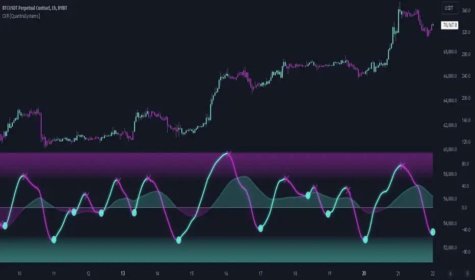
Cosine Kernel Regressions [QuantraSystems]Cosine Kernel Regressions
Introduction
The Cosine Kernel Regressions indicator (CKR) uses mathematical concepts to offer a unique approach to market analysis. This indicator employs Kernel Regressions using bespoke tunable Cosine functions in order to smoothly interpret a variety of market data, providing traders with incredibly clean insights into market trends.
The CKR is particularly useful for traders looking to understand underlying trends without the 'noise' typical in raw price movements. It can serve as a standalone trend analysis tool or be combined with other indicators for more robust trading strategies.
Legend
Fast Trend Signal Line - This is the foreground oscillator, it is colored upon the earliest confirmation of a change in trend direction.
Slow Trend Signal Line - This oscillator is calculated in a similar manner. However, it utilizes a lower frequency within the cosine tuning function, allowing it to capture longer and broader trends in one signal. This allows for tactical trading; the user can trade smaller moves without losing sight of the broader trend.
Case Study
In this case study, the CKR was used alongside the Triple Confirmation Kernel Regression Oscillator (KRO)
Initially, the KRO indicated an oversold condition, which could be interpreted as a signal to enter a long position in anticipation of a price rebound. However, the CKR’s fast trend signal line had not yet confirmed a positive trend direction - suggesting that entering a trade too early and without confirmation could be a mistake.
Waiting for a confirmed positive trend from the CKR proved beneficial for this trade. A few candles after the oversold signal, the CKR's fast trend signal line shifted upwards, indicating a strong upward momentum. This was the optimal entry point suggested by the CKR, occurring after the confirmation of the trend change, which significantly reduced the likelihood of entering during a false recovery or continuation of the downtrend.
This is one of the many uses of the CKR - by timing entries using the fast signal line , traders could avoid unnecessary losses by preventing premature entries.
Methodology
The methodology behind CKR is a multi-layered approach and utilizes many ‘base’ indicators.
Relative Strength Index
Stochastic Oscillator
Bollinger Band Percent
Chande Momentum Oscillator
Commodity Channel Index
Fisher Transform
Volume Zone Oscillator
The calculated output from each indicator is standardized and scaled before being averaged. This prevents any single indicator from overpowering the resulting signal.
// ╔════════════════════════════════╗ //
// ║ Scaling/Range Adjustment ║ //
// ╚════════════════════════════════╝ //
RSI_ReScale (_res ) => ( _res - 50 ) * 2.8
STOCH_ReScale (_stoch ) => ( _stoch - 50 ) * 2
BBPCT_ReScale (_bbpct ) => ( _bbpct - 0.5 ) * 120
CMO_ReScale (_chandeMO ) => ( _chandeMO * 1.15 )
CCI_ReScale (_cci ) => ( _cci / 2 )
FISH_ReScale (_fish1 ) => ( _fish1 * 30 )
VZO_ReScale (_VP, _TV ) => (_VP / _TV) * 110
These outputs are then fed into a customized cosine kernel regression function, which smooths the data, and combines all inputs into a single coherent output.
// ╔════════════════════════════════╗ //
// ║ COSINE KERNEL REGRESSIONS ║ //
// ╚════════════════════════════════╝ //
// Define a function to compute the cosine of an input scaled by a frequency tuner
cosine(x, z) =>
// Where x = source input
// y = function output
// z = frequency tuner
var y = 0.
y := math.cos(z * x)
Y
// Define a kernel that utilizes the cosine function
kernel(x, z) =>
var y = 0.
y := cosine(x, z)
math.abs(x) <= math.pi/(2 * z) ? math.abs(y) : 0. // cos(zx) = 0
// The above restricts the wave to positive values // when x = π / 2z
The tuning of the regression is adjustable, allowing users to fine-tune the sensitivity and responsiveness of the indicator to match specific trading strategies or market conditions. This robust methodology ensures that CKR provides a reliable and adaptable tool for market analysis.
Pine Script Chart ViewerDisplay your custom charts exported from anywhere in TradingView.
Put your candles on candles :
var Candle candles = array.from(...)
For instance:
var Candle candles = array.from(Candle.new(2.0, 4.0, 1.0, 3.0), Candle.new(3.0, 5.0, 2.0, 4.0))
Candle details:
Candle.new(open_1, high_1, low_1, close_1)

Price Cross Time Custom Range Interactive█ OVERVIEW
This indicator was a time-based indicator and intended as educational purpose only based on pine script v5 functions for ta.cross() , ta.crossover() and ta.crossunder() .
I realised that there is some overlap price with the cross functions, hence I integrate them into Custom Range Interactive with value variance and overlap displayed into table.
This was my submission for Pinefest #1 , I decided to share this as public, I may accidentally delete this as long as i keep as private.
█ INSPIRATION
Inspired by design, code and usage of CAGR. Basic usage of custom range / interactive, pretty much explained here . Credits to TradingView.
█ FEATURES
1. Custom Range Interactive
2. Label can be resize and change color.
3. Label show tooltip for price and time.
4. Label can be offset to improve readability.
5. Table can show price variance when any cross is true.
6. Table can show overlap if found crosss is overlap either with crossover and crossunder.
7. Table text color automatically change based on chart background (light / dark mode).
8. Source 2 is drawn as straight line, while Source 1 will draw as label either above line for crossover, below line for crossunder and marked 'X' if crossing with Source 2's line.
9. Cross 'X' label can be offset to improve readability.
10. Both Source 1 and Source 2 can select Open, Close, High and Low, which can be displayed into table.
█ LIMITATIONS
1. Table is limited to intraday timeframe only as time format is not accurate for daily timeframe and above. Example daily timeframe will give result less 1 day from actual date.
2. I did not include other sources such external source or any built in sources such as hl2, hlc3, ohlc4 and hlcc4.
█ CODE EXPLAINATION
I pretty much create custom function with method which returns tuple value.
method crossVariant(float price = na, chart.point ref = na) =>
cross = ta.cross( price, ref.price)
over = ta.crossover( price, ref.price)
under = ta.crossunder(price, ref.price)
Unfortunately, I unable make the labels into array which i plan to return string value by getting the text value from array label, hence i use label.all and add incremental int value as reference.
series label labelCross = na, labelCross.delete()
var int num = 0
if over
num += 1
labelCross := label.new()
if under
num += 1
labelCross := label.new()
if cross
num += 1
labelCross := label.new()
I realised cross value can be overlap with crossover and crossunder, hence I add bool to enable force overlap and add additional bools.
series label labelCross = na, labelCross.delete()
var int num = 0
if forceOverlap
if over
num += 1
labelCross := label.new()
if under
num += 1
labelCross := label.new()
if cross
num += 1
labelCross := label.new()
else
if cross and over
num += 1
labelCross := label.new()
if cross and under
num += 1
labelCross := label.new()
if cross and not over and not under
num += 1
labelCross := label.new()
█ USAGE / EXAMPLES

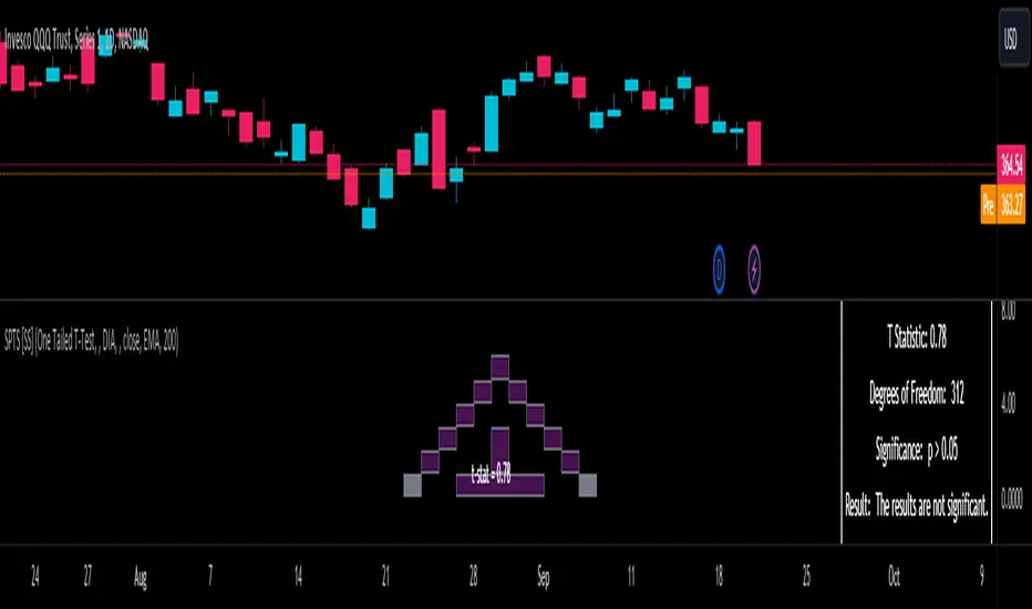
Statistical Package for the Trading Sciences [SS]
This is SPTS.
It stands for Statistical Package for the Trading Sciences.
Its a play on SPSS (Statistical Package for the Social Sciences) by IBM (software that, prior to Pinescript, I would use on a daily basis for trading).
Let's preface this indicator first:
This isn't so much an indicator as it is a project. A passion project really.
This has been in the works for months and I still feel like its incomplete. But the plan here is to continue to add functionality to it and actually have the Pinecoding and Tradingview community contribute to it.
As a math based trader, I relied on Excel, SPSS and R constantly to plan my trades. Since learning a functional amount of Pinescript and coding a lot of what I do and what I relied on SPSS, Excel and R for, I use it perhaps maybe a few times a week.
This indicator, or package, has some of the key things I used Excel and SPSS for on a daily and weekly basis. This also adds a lot of, I would say, fairly complex math functionality to Pinescript. Because this is adding functionality not necessarily native to Pinescript, I have placed most, if not all, of the functionality into actual exportable functions. I have also set it up as a kind of library, with explanations and tips on how other coders can take these functions and implement them into other scripts.
The hope here is that other coders will take it, build upon it, improve it and hopefully share additional functionality that can be added into this package. Hence why I call it a project. Okay, let's get into an overview:
Current Functions of SPTS:
SPTS currently has the following functionality (further explanations will be offered below):
Ability to Perform a One-Tailed, Two-Tailed and Paired Sample T-Test, with corresponding P value.
Standard Pearson Correlation (with functionality to be able to calculate the Pearson Correlation between 2 arrays).
Quadratic (or Curvlinear) correlation assessments.
R squared Assessments.
Standard Linear Regression.
Multiple Regression of 2 independent variables.
Tests of Normality (with Kurtosis and Skewness) and recognition of up to 7 Different Distributions.
ARIMA Modeller (Sort of, more details below)
Okay, so let's go over each of them!
T-Tests
So traditionally, most correlation assessments on Pinescript are done with a generic Pearson Correlation using the "ta.correlation" argument. However, this is not always the best test to be used for correlations and determine effects. One approach to correlation assessments used frequently in economics is the T-Test assessment.
The t-test is a statistical hypothesis test used to determine if there is a significant difference between the means of two groups. It assesses whether the sample means are likely to have come from populations with the same mean. The test produces a t-statistic, which is then compared to a critical value from the t-distribution to determine statistical significance. Lower p-values indicate stronger evidence against the null hypothesis of equal means.
A significant t-test result, indicating the rejection of the null hypothesis, suggests that there is statistical evidence to support that there is a significant difference between the means of the two groups being compared. In practical terms, it means that the observed difference in sample means is unlikely to have occurred by random chance alone. Researchers typically interpret this as evidence that there is a real, meaningful difference between the groups being studied.
Some uses of the T-Test in finance include:
Risk Assessment: The t-test can be used to compare the risk profiles of different financial assets or portfolios. It helps investors assess whether the differences in returns or volatility are statistically significant.
Pairs Trading: Traders often apply the t-test when engaging in pairs trading, a strategy that involves trading two correlated securities. It helps determine when the price spread between the two assets is statistically significant and may revert to the mean.
Volatility Analysis: Traders and risk managers use t-tests to compare the volatility of different assets or portfolios, assessing whether one is significantly more or less volatile than another.
Market Efficiency Tests: Financial researchers use t-tests to test the Efficient Market Hypothesis by assessing whether stock price movements follow a random walk or if there are statistically significant deviations from it.
Value at Risk (VaR) Calculation: Risk managers use t-tests to calculate VaR, a measure of potential losses in a portfolio. It helps assess whether a portfolio's value is likely to fall below a certain threshold.
There are many other applications, but these are a few of the highlights. SPTS permits 3 different types of T-Test analyses, these being the One Tailed T-Test (if you want to test a single direction), two tailed T-Test (if you are unsure of which direction is significant) and a paired sample t-test.
Which T is the Right T?
Generally, a one-tailed t-test is used to determine if a sample mean is significantly greater than or less than a specified population mean, whereas a two-tailed t-test assesses if the sample mean is significantly different (either greater or less) from the population mean. In contrast, a paired sample t-test compares two sets of paired observations (e.g., before and after treatment) to assess if there's a significant difference in their means, typically used when the data points in each pair are related or dependent.
So which do you use? Well, it depends on what you want to know. As a general rule a one tailed t-test is sufficient and will help you pinpoint directionality of the relationship (that one ticker or economic indicator has a significant affect on another in a linear way).
A two tailed is more broad and looks for significance in either direction.
A paired sample t-test usually looks at identical groups to see if one group has a statistically different outcome. This is usually used in clinical trials to compare treatment interventions in identical groups. It's use in finance is somewhat limited, but it is invaluable when you want to compare equities that track the same thing (for example SPX vs SPY vs ES1!) or you want to test a hypothesis about an index and a leveraged share (for example, the relationship between FNGU and, say, MSFT or NVDA).
Statistical Significance
In general, with a t-test you would need to reference a T-Table to determine the statistical significance of the degree of Freedom and the T-Statistic.
However, because I wanted Pinescript to full fledge replace SPSS and Excel, I went ahead and threw the T-Table into an array, so that Pinescript can make the determination itself of the actual P value for a t-test, no cross referencing required :-).
Left tail (Significant):
Both tails (Significant):
Distributed throughout (insignificant):
As you can see in the images above, the t-test will also display a bell-curve analysis of where the significance falls (left tail, both tails or insignificant, distributed throughout).
That said, I have not included this function for the paired sample t-test because that is a bit more nuanced. But for the one and two tailed assessments, the indicator will provide you the P value.
Pearson Correlation Assessment
I don't think I need to go into too much detail on this one.
I have put in functionality to quickly calculate the Pearson Correlation of two array's, which is not currently possible with the "ta.correlation" function.
Quadratic (Curvlinear) Correlation
Not everything in life is linear, sometimes things are curved!
The Pearson Correlation is great for linear assessments, but tends to under-estimate the degree of the relationship in curved relationships. There currently is no native function to t-test for quadratic/curvlinear relationships, so I went ahead and created one.
You can see an example of how Quadratic and Pearson Correlations vary when you look at CME_MINI:ES1! against AMEX:DIA for the past 10 ish months:
Pearson Correlation:
Quadratic Correlation:
One or the other is not always the best, so it is important to check both!
R-Squared Assessments:
The R-squared value, or the square of the Pearson correlation coefficient (r), is used to measure the proportion of variance in one variable that can be explained by the linear relationship with another variable. It represents the goodness-of-fit of a linear regression model with a single predictor variable.
R-Squared is offered in 3 separate forms within this indicator. First, there is the generic R squared which is taking the square root of a Pearson Correlation assessment to assess the variance.
The next is the R-Squared which is calculated from an actual linear regression model done within the indicator.
The first is the R-Squared which is calculated from a multiple regression model done within the indicator.
Regardless of which R-Squared value you are using, the meaning is the same. R-Square assesses the variance between the variables under assessment and can offer an insight into the goodness of fit and the ability of the model to account for the degree of variance.
Here is the R Squared assessment of the SPX against the US Money Supply:
Standard Linear Regression
The indicator contains the ability to do a standard linear regression model. You can convert one ticker or economic indicator into a stock, ticker or other economic indicator. The indicator will provide you with all of the expected information from a linear regression model, including the coefficients, intercept, error assessments, correlation and R2 value.
Here is AAPL and MSFT as an example:
Multiple Regression
Oh man, this was something I really wanted in Pinescript, and now we have it!
I have created a function for multiple regression, which, if you export the function, will permit you to perform multiple regression on any variables available in Pinescript!
Using this functionality in the indicator, you will need to select 2, dependent variables and a single independent variable.
Here is an example of multiple regression for NASDAQ:AAPL using NASDAQ:MSFT and NASDAQ:NVDA :
And an example of SPX using the US Money Supply (M2) and AMEX:GLD :
Tests of Normality:
Many indicators perform a lot of functions on the assumption of normality, yet there are no indicators that actually test that assumption!
So, I have inputted a function to assess for normality. It uses the Kurtosis and Skewness to determine up to 7 different distribution types and it will explain the implication of the distribution. Here is an example of SP:SPX on the Monthly Perspective since 2010:
And NYSE:BA since the 60s:
And NVDA since 2015:
ARIMA Modeller
Okay, so let me disclose, this isn't a full fledge ARIMA modeller. I took some shortcuts.
True ARIMA modelling would involve decomposing the seasonality from the trend. I omitted this step for simplicity sake. Instead, you can select between using an EMA or SMA based approach, and it will perform an autogressive type analysis on the EMA or SMA.
I have tested it on lookback with results provided by SPSS and this actually works better than SPSS' ARIMA function. So I am actually kind of impressed.
You will need to input your parameters for the ARIMA model, I usually would do a 14, 21 and 50 day EMA of the close price, and it will forecast out that range over the length of the EMA.
So for example, if you select the EMA 50 on the daily, it will plot out the forecast for the next 50 days based on an autoregressive model created on the EMA 50. Here is how it looks on AMEX:SPY :
You can also elect to plot the upper and lower confidence bands:
Closing Remarks
So that is the indicator/package.
I do hope to continue expanding its functionality, but as of now, it does already have quite a lot of functionality.
I really hope you enjoy it and find it helpful. This. Has. Taken. AGES! No joke. Between referencing my old statistics textbooks, trying to remember how to calculate some of these things, and wanting to throw my computer against the wall because of errors in the code, this was a task, that's for sure. So I really hope you find some usefulness in it all and enjoy the ability to be able to do functions that previously could really only be done in external software.
As always, leave your comments, suggestions and feedback below!
Take care!
libHTF[without request.security()]Library "libHTF"
libHTF: use HTF values without request.security()
This library enables to use HTF candles without request.security().
Basic data structure
Using to access values in the same manner as series variable.
The last member of HTF array is always latest current TF's data.
If new bar in HTF(same as last bar closes), new member is pushed to HTF array.
2nd from the last member of HTF array is latest fixed(closed) bar.
HTF: How to use
1. set TF
tf_higher() function selects higher TF. TF steps are ("1","5","15","60","240","D","W","M","3M","6M","Y").
example:
tfChart = timeframe.period
htf1 = tf_higher(tfChart)
2. set HTF matrix
htf_candle() function returns 1 bool and 1 matrix.
bool is a flag for start of new candle in HTF context.
matrix is HTF candle data(0:open,1:time_open,2:close,3:time_close,4:high,5:time:high,6:low,7:time_low).
example:
=htf_candle(htf1)
3. how to access HTF candle data
you can get values using .lastx() method.
please be careful, return value is always float evenif it is "time". you need to cast to int time value when using for xloc.bartime.
example:
htf1open=m1.lastx("open")
htf1close=m1.lastx("close")
//if you need to use histrical value.
lastopen=open
lasthtf1open=m1.lastx("open",1)
4. how to store Data of HTF context
you have to use array to store data of HTF context.
array.htf_push() method handles the last member of array. if new_bar in HTF, it push new member. otherwise it set value to the last member.
example:
array a_close=array.new(1,na)
a_close.htf_push(b_new_bar1,m1.lastx("close"))
HTFsrc: How to use
1. how to setup src.
set_src() function is set current tf's src from string(open/high/low/close/hl2/hlc3/ohlc4/hlcc4).
set_htfsrc() function returns src array of HTF candle.
example:
_src="ohlc4"
src=set_src(_src)
htf1src=set_htfsrc(_src,b_new_bar1,m1)
(if you need to use HTF src in series float)
s_htf1src=htf1src.lastx()
HighLow: How to use
1. set HTF arrays
highlow() and htfhighlow() function calculates high/low and return high/low prices and time.
the functions return 1 int and 8arrays.
int is a flag for new high(1) or new low(-1).
arrays are high/low and return high/low data. float for price, int for time.
example
=
highlow()
=
htfhighlow(m1)
2. how to access HighLow data
you can get values using .lastx() method.
example:
if i_renew==1
myhigh=a_high.lastx()
//if you need to use histrical value.
myhigh=a_high.lastx(1)
other functions
functions for HTF candle matrix or HTF src array in this script are
htf_sma()/htf_ema()/htf_rma()
htf_rsi()/htf_rci()/htf_dmi()
method lastx(arrayid, lastindex)
method like array.last. it returns lastindex from the last member, if parameter is set.
Namespace types: float
Parameters:
arrayid (float )
lastindex (int) : (int) default value is "0"(the last member). if you need to access historical value, increment it(same manner as series vars).
Returns: float value of lastindex from the last member of the array. returns na, if fail.
method lastx(arrayid, lastindex)
method like array.last. it returns lastindex from the last member, if parameter is set.
Namespace types: int
Parameters:
arrayid (int )
lastindex (int) : (int) default value is "0"(the last member). if you need to access historical value, increment it(same manner as series vars).
Returns: int value of lastindex from the last member of the array. returns na, if fail.
method lastx(m, _type, lastindex)
method for handling htf matrix.
Namespace types: matrix
Parameters:
m (matrix) : (matrix) matrix for htf candle.
_type (string) : (string) value type of htf candle:
lastindex (int) : (int) default value is "0"(the last member).
Returns: (float) value of htf candle. (caution: need to cast float to int to use time values!)
method set_last(arrayid, val)
method to set a value of the last member of the array. it sets value to the last member.
Namespace types: float
Parameters:
arrayid (float )
val (float) : (float) value to set.
Returns: nothing
method htf_push(arrayid, b, val)
method to push new member to htf context. if new bar in htf, it works as push. else it works as set_last.
Namespace types: float
Parameters:
arrayid (float )
b (bool) : (bool) true:push,false:set_last
val (float) : (float) _f the value to set.
Returns: nothing
method tf_higher(tf)
method to set higher tf from tf string. TF steps are .
Namespace types: series string, simple string, input string, const string
Parameters:
tf (string) : (string) tf string
Returns: (string) string of higher tf.
htf_candle(_tf, _TZ)
build htf candles
Parameters:
_tf (string) : (string) tf string.
_TZ (string) : of timezone. default value is "GMT+3".
Returns: bool for new bar@htf and matrix for snapshot of htf candle
set_src(_src_type)
set src.
Parameters:
_src_type (string) : (string) type of source:
Returns: (series float) src value
set_htfsrc(_src_type, _nb, _m)
set htf src.
Parameters:
_src_type (string) : (string) type of source:
_nb (bool) : (bool) flag of new bar
_m (matrix) : (matrix) matrix for htf candle.
Returns: (array) array of src value
is_up()
last_is_up()
peak_bottom(_latest, _last)
Parameters:
_latest (bool)
_last (bool)
htf_is_up(_m)
Parameters:
_m (matrix)
htf_last_is_up(_m)
Parameters:
_m (matrix)
highlow(_b_bartime_price)
Parameters:
_b_bartime_price (bool)
htfhighlow(_m, _b_bartime_price)
Parameters:
_m (matrix)
_b_bartime_price (bool)
htf_sma(_a_src, _len)
Parameters:
_a_src (float )
_len (int)
htf_rma(_a_src, _new_bar, _len)
Parameters:
_a_src (float )
_new_bar (bool)
_len (int)
htf_ema(_a_src, _new_bar, _len)
Parameters:
_a_src (float )
_new_bar (bool)
_len (int)
htf_rsi(_a_src, _new_bar, _len)
Parameters:
_a_src (float )
_new_bar (bool)
_len (int)
rci(_src, _len)
Parameters:
_src (float)
_len (int)
htf_rci(_a_src, _len)
Parameters:
_a_src (float )
_len (int)
htf_dmi(_m, _new_bar, _len, _ma_type)
Parameters:
_m (matrix)
_new_bar (bool)
_len (int)
_ma_type (string)

JavaScript-style Debug ConsoleThis library provides a JavaScript-style debug console to Pine Coders. It supports the most commonly used utilities from the WHATWG Console Standard including the following:
• console.log
• console.debug
• console.info
• console.warn
• console.error
• console.assert
• console.count
• console.countReset
• console.group
• console.groupEnd
• console.clear
In addition to the WHATWG standard, this library also supports the following methods:
• console.show
• console.hide
FEATURES
• Follows the WHATWG Console Standard, which is widely adopted by all major JavaScript runtimes including browsers and Node.js.
• Provides an out-of-box UI with pre-configured theming, ensuring a clean and professional-looking console.
• Allows for easy UI customizations to fit your personal preferences.
• Has extremely simple import and initialization, making it easy to integrate with your existing codebase.
USAGE
1. Import this library:
import algotraderdev/Console/1
2. Initialize the console object:
var console = Console.new()
// You can also specify optional params to customize the look & feel.
var console = Console.new(
position = position.bottom_right,
max_rows = 50,
width = 0,
text_size = size.normal,
background_color = #000000CC,
timestamp_color = #AAAAAA,
info_message_color = #DDDDDD,
debug_message_color = #AAAAAA,
warn_message_color = #FFEB3B,
error_message_color = #ff3c00)
3. Use the console object to debug your code. Here are some examples:
// Basic logging
console.log('hello world!') // prints 'hello world'
console.warn('warn') // prints 'warn' in yellow
console.error('error') // prints 'error' in red
console.clear() // clears the console
// Assertion
console.assert(a.isEmpty(), 'array should be empty') // prints 'assertion failed: array should be empty' if the array is not empty
// Counter
console.count('fooFunction') // prints 'fooFunction: 1'
console.count('fooFunction') // prints 'fooFunction: 2'
console.countReset('fooFunction') // resets the counter
console.count('fooFunction') // prints 'fooFunction: 1'
// Group
console.log('A')
console.group()
console.log('B')
console.group()
console.log('C')
console.log('D')
console.groupEnd()
console.log('E')
console.groupEnd()
console.log('F')
// prints
// A
// B
// C
// D
// E
// F
// Hide and show
console.hide()
console.show()
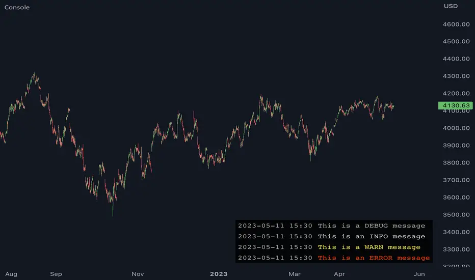
libhs.log.DEMO◼ Overview
This is a demonstration of dual logging library I have ported from my personal use for public use. Please start bar replay from Bar#4, and progress automatically slowly or manually.You would need to go through 450+ bars to see the full capability.
Logger=A dual logging library for developers. Tradingview lacks logging capability. This library provided logging while developing your scripts and is to be used by developers when developing and debugging their scripts.
Using this library would potentially slow down you scripts. Hence, use this for debugging only. Once your code is as you would like it to be, remove the logging code.
◼︎ Usage (Console):
Console = A sleek single cell logging with a limit of 4096 characters. When you dont need a large logging capability.
//@version=5
indicator("demo.Console", overlay=true)
plot(na)
import GETpacman/log/2 as logger
var console = logger.log.new()
console.init() // init() should be called as first line after variable declaration
console.FrameColor:=color.green
console.log('\n')
console.log('\n')
console.log('Hello World')
console.log('\n')
console.log('\n')
console.ShowStatusBar:=true
console.StatusBarAtBottom:=true
console.FrameColor:=color.blue //settings can be changed anytime before show method is called. Even twice. The last call will set the final value
console.ShowHeader:=false //this wont throw error but is not used for console
console.show(position=position.bottom_right) //this should be the last line of your code, after all methods and settings have been dealt with.
◼︎ Usage (Logx):
Logx = Multiple columns logging with a limit of 4096 characters each message. When you need to log large number of messages.
//@version=5
indicator("demo.Logx", overlay=true)
plot(na)
import GETpacman/log/2 as logger
var logx = logger.log.new()
logx.init() // init() should be called as first line after variable declaration
logx.FrameColor:=color.green
logx.log('\n')
logx.log('\n')
logx.log('Hello World')
logx.log('\n')
logx.log('\n')
logx.ShowStatusBar:=true
logx.StatusBarAtBottom:=true
logx.ShowQ3:=false
logx.ShowQ4:=false
logx.ShowQ5:=false
logx.ShowQ6:=false
logx.FrameColor:=color.olive //settings can be changed anytime before show method is called. Even twice. The last call will set the final value
logx.show(position=position.top_right) //this should be the last line of your code, after all methods and settings have been dealt with.
◼︎ Fields (with default settings)
▶︎ IsConsole = True Log will act as Console if true, otherwise it will act as Logx
▶︎ ShowHeader = True (Log only) Will show a header at top or bottom of logx.
▶︎ HeaderAtTop = True (Log only) Will show the header at the top, or bottom if false, if ShowHeader is true.
▶︎ ShowStatusBar = True Will show a status bar at the bottom
▶︎ StatusBarAtBottom = True Will show the status bar at the bottom, or top if false, if ShowHeader is true.
▶︎ ShowMetaStatus = True Will show the meta info within status bar (Current Bar, characters left in console, Paging On Every Bar, Console dumped data etc)
▶︎ ShowBarIndex = True Logx will show column for Bar Index when the message was logged. Console will add Bar index at the front of logged messages
▶︎ ShowDateTime = True Logx will show column for Date/Time passed with the logged message logged. Console will add Date/Time at the front of logged messages
▶︎ ShowLogLevels = True Logx will show column for Log levels corresponding to error codes. Console will log levels in the status bar
▶︎ ReplaceWithErrorCodes = True (Log only) Logx will show error codes instead of log levels, if ShowLogLevels is switched on
▶︎ RestrictLevelsToKey7 = True Log levels will be restricted to Ley 7 codes - TRACE, DEBUG, INFO, WARNING, ERROR, CRITICAL, FATAL
▶︎ ShowQ1 = True (Log only) Show the column for Q1
▶︎ ShowQ2 = True (Log only) Show the column for Q2
▶︎ ShowQ3 = True (Log only) Show the column for Q3
▶︎ ShowQ4 = True (Log only) Show the column for Q4
▶︎ ShowQ5 = True (Log only) Show the column for Q5
▶︎ ShowQ6 = True (Log only) Show the column for Q6
▶︎ ColorText = True Log/Console will color text as per error codes
▶︎ HighlightText = True Log/Console will highlight text (like denoting) as per error codes
▶︎ AutoMerge = True (Log only) Merge the queues towards the right if there is no data in those queues.
▶︎ PageOnEveryBar = True Clear data from previous bars on each new bar, in conjuction with PageHistory setting.
▶︎ MoveLogUp = True Move log in up direction. Setting to false will push logs down.
▶︎ MarkNewBar = True On each change of bar, add a marker to show the bar has changed
▶︎ PrefixLogLevel = True (Console only) Prefix all messages with the log level corresponding to error code.
▶︎ MinWidth = 40 Set the minimum width needed to be seen. Prevents logx/console shrinking below these number of characters.
▶︎ TabSizeQ1 = 0 If set to more than one, the messages on Q1 or Console messages will indent by this size based on error code (Max 4 used)
▶︎ TabSizeQ2 = 0 If set to more than one, the messages on Q2 will indent by this size based on error code (Max 4 used)
▶︎ TabSizeQ3 = 0 If set to more than one, the messages on Q2 will indent by this size based on error code (Max 4 used)
▶︎ TabSizeQ4 = 0 If set to more than one, the messages on Q2 will indent by this size based on error code (Max 4 used)
▶︎ TabSizeQ5 = 0 If set to more than one, the messages on Q2 will indent by this size based on error code (Max 4 used)
▶︎ TabSizeQ6 = 0 If set to more than one, the messages on Q2 will indent by this size based on error code (Max 4 used)
▶︎ PageHistory = 0 Used with PageOnEveryBar. Determines how many historial pages to keep.
▶︎ HeaderQbarIndex = 'Bar#' (Logx only) The header to show for Bar Index
▶︎ HeaderQdateTime = 'Date' (Logx only) The header to show for Date/Time
▶︎ HeaderQerrorCode = 'eCode' (Logx only) The header to show for Error Codes
▶︎ HeaderQlogLevel = 'State' (Logx only) The header to show for Log Level
▶︎ HeaderQ1 = 'h.Q1' (Logx only) The header to show for Q1
▶︎ HeaderQ2 = 'h.Q2' (Logx only) The header to show for Q2
▶︎ HeaderQ3 = 'h.Q3' (Logx only) The header to show for Q3
▶︎ HeaderQ4 = 'h.Q4' (Logx only) The header to show for Q4
▶︎ HeaderQ5 = 'h.Q5' (Logx only) The header to show for Q5
▶︎ HeaderQ6 = 'h.Q6' (Logx only) The header to show for Q6
▶︎ Status = '' Set the status to this text.
▶︎ HeaderColor Set the color for the header
▶︎ HeaderColorBG Set the background color for the header
▶︎ StatusColor Set the color for the status bar
▶︎ StatusColorBG Set the background color for the status bar
▶︎ TextColor Set the color for the text used without error code or code 0.
▶︎ TextColorBG Set the background color for the text used without error code or code 0.
▶︎ FrameColor Set the color for the frame around Logx/Console
▶︎ FrameSize = 1 Set the size of the frame around Logx/Console
▶︎ CellBorderSize = 0 Set the size of the border around cells.
▶︎ CellBorderColor Set the color for the border around cells within Logx/Console
▶︎ SeparatorColor = gray Set the color of separate in between Console/Logx Attachment
◼︎ Methods (summary)
● init ▶︎ Initialise the log
● log ▶︎ Log the messages. Use method show to display the messages
● page ▶︎ Clear messages from previous bar while logging messages on this bar.
● show ▶︎ Shows a table displaying the logged messages
● clear ▶︎ Clears the log of all messages
● resize ▶︎ Resizes the log. If size is for reduction then oldest messages are lost first.
● turnPage ▶︎ When called, all messages marked with previous page, or from start are cleared
● dateTimeFormat ▶︎ Sets the date time format to be used when displaying date/time info.
● resetTextColor ▶︎ Reset Text Color to library default
● resetTextBGcolor ▶︎ Reset Text BG Color to library default
● resetHeaderColor ▶︎ Reset Header Color to library default
● resetHeaderBGcolor ▶︎ Reset Header BG Color to library default
● resetStatusColor ▶︎ Reset Status Color to library default
● resetStatusBGcolor ▶︎ Reset Status BG Color to library default
● setColors ▶︎ Sets the colors to be used for corresponding error codes
● setColorsBG ▶︎ Sets the background colors to be used for corresponding error codes. If not match of error code, then text color used.
● setColorsHC ▶︎ Sets the highlight colors to be used for corresponding error codes.If not match of error code, then text bg color used.
● resetColors ▶︎ Reset the colors to library default (Total 36, not including error code 0)
● resetColorsBG ▶︎ Reset the background colors to library default
● resetColorsHC ▶︎ Reset the highlight colors to library default
● setLevelNames ▶︎ Set the log level names to be used for corresponding error codes. If not match of error code, then empty string used.
● resetLevelNames ▶︎ Reset the log level names to library default. (Total 36) 1=TRACE, 2=DEBUG, 3=INFO, 4=WARNING, 5=ERROR, 6=CRITICAL, 7=FATAL
● attach ▶︎ Attaches a console to an existing Logx, allowing to have dual logging system independent of each other
● detach ▶︎ Detaches an already attached console from Logx
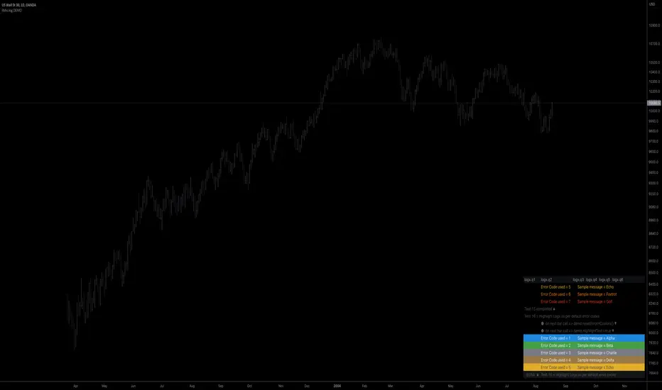
loggerLibrary "logger"
◼ Overview
A dual logging library for developers. Tradingview lacks logging capability. This library provides logging while developing your scripts and is to be used by developers when developing and debugging their scripts.
Using this library would potentially slow down you scripts. Hence, use this for debugging only. Once your code is as you would like it to be, remove the logging code.
◼︎ Usage (Console):
Console = A sleek single cell logging with a limit of 4096 characters. When you dont need a large logging capability.
//@version=5
indicator("demo.Console", overlay=true)
plot(na)
import GETpacman/logger/1 as logger
var console = logger.log.new()
console.init() // init() should be called as first line after variable declaration
console.FrameColor:=color.green
console.log('\n')
console.log('\n')
console.log('Hello World')
console.log('\n')
console.log('\n')
console.ShowStatusBar:=true
console.StatusBarAtBottom:=true
console.FrameColor:=color.blue //settings can be changed anytime before show method is called. Even twice. The last call will set the final value
console.ShowHeader:=false //this wont throw error but is not used for console
console.show(position=position.bottom_right) //this should be the last line of your code, after all methods and settings have been dealt with.
◼︎ Usage (Logx):
Logx = Multiple columns logging with a limit of 4096 characters each message. When you need to log large number of messages.
//@version=5
indicator("demo.Logx", overlay=true)
plot(na)
import GETpacman/logger/1 as logger
var logx = logger.log.new()
logx.init() // init() should be called as first line after variable declaration
logx.FrameColor:=color.green
logx.log('\n')
logx.log('\n')
logx.log('Hello World')
logx.log('\n')
logx.log('\n')
logx.ShowStatusBar:=true
logx.StatusBarAtBottom:=true
logx.ShowQ3:=false
logx.ShowQ4:=false
logx.ShowQ5:=false
logx.ShowQ6:=false
logx.FrameColor:=color.olive //settings can be changed anytime before show method is called. Even twice. The last call will set the final value
logx.show(position=position.top_right) //this should be the last line of your code, after all methods and settings have been dealt with.
◼︎ Fields (with default settings)
▶︎ IsConsole = True Log will act as Console if true, otherwise it will act as Logx
▶︎ ShowHeader = True (Log only) Will show a header at top or bottom of logx.
▶︎ HeaderAtTop = True (Log only) Will show the header at the top, or bottom if false, if ShowHeader is true.
▶︎ ShowStatusBar = True Will show a status bar at the bottom
▶︎ StatusBarAtBottom = True Will show the status bar at the bottom, or top if false, if ShowHeader is true.
▶︎ ShowMetaStatus = True Will show the meta info within status bar (Current Bar, characters left in console, Paging On Every Bar, Console dumped data etc)
▶︎ ShowBarIndex = True Logx will show column for Bar Index when the message was logged. Console will add Bar index at the front of logged messages
▶︎ ShowDateTime = True Logx will show column for Date/Time passed with the logged message logged. Console will add Date/Time at the front of logged messages
▶︎ ShowLogLevels = True Logx will show column for Log levels corresponding to error codes. Console will log levels in the status bar
▶︎ ReplaceWithErrorCodes = True (Log only) Logx will show error codes instead of log levels, if ShowLogLevels is switched on
▶︎ RestrictLevelsToKey7 = True Log levels will be restricted to Ley 7 codes - TRACE, DEBUG, INFO, WARNING, ERROR, CRITICAL, FATAL
▶︎ ShowQ1 = True (Log only) Show the column for Q1
▶︎ ShowQ2 = True (Log only) Show the column for Q2
▶︎ ShowQ3 = True (Log only) Show the column for Q3
▶︎ ShowQ4 = True (Log only) Show the column for Q4
▶︎ ShowQ5 = True (Log only) Show the column for Q5
▶︎ ShowQ6 = True (Log only) Show the column for Q6
▶︎ ColorText = True Log/Console will color text as per error codes
▶︎ HighlightText = True Log/Console will highlight text (like denoting) as per error codes
▶︎ AutoMerge = True (Log only) Merge the queues towards the right if there is no data in those queues.
▶︎ PageOnEveryBar = True Clear data from previous bars on each new bar, in conjuction with PageHistory setting.
▶︎ MoveLogUp = True Move log in up direction. Setting to false will push logs down.
▶︎ MarkNewBar = True On each change of bar, add a marker to show the bar has changed
▶︎ PrefixLogLevel = True (Console only) Prefix all messages with the log level corresponding to error code.
▶︎ MinWidth = 40 Set the minimum width needed to be seen. Prevents logx/console shrinking below these number of characters.
▶︎ TabSizeQ1 = 0 If set to more than one, the messages on Q1 or Console messages will indent by this size based on error code (Max 4 used)
▶︎ TabSizeQ2 = 0 If set to more than one, the messages on Q2 will indent by this size based on error code (Max 4 used)
▶︎ TabSizeQ3 = 0 If set to more than one, the messages on Q2 will indent by this size based on error code (Max 4 used)
▶︎ TabSizeQ4 = 0 If set to more than one, the messages on Q2 will indent by this size based on error code (Max 4 used)
▶︎ TabSizeQ5 = 0 If set to more than one, the messages on Q2 will indent by this size based on error code (Max 4 used)
▶︎ TabSizeQ6 = 0 If set to more than one, the messages on Q2 will indent by this size based on error code (Max 4 used)
▶︎ PageHistory = 0 Used with PageOnEveryBar. Determines how many historial pages to keep.
▶︎ HeaderQbarIndex = 'Bar#' (Logx only) The header to show for Bar Index
▶︎ HeaderQdateTime = 'Date' (Logx only) The header to show for Date/Time
▶︎ HeaderQerrorCode = 'eCode' (Logx only) The header to show for Error Codes
▶︎ HeaderQlogLevel = 'State' (Logx only) The header to show for Log Level
▶︎ HeaderQ1 = 'h.Q1' (Logx only) The header to show for Q1
▶︎ HeaderQ2 = 'h.Q2' (Logx only) The header to show for Q2
▶︎ HeaderQ3 = 'h.Q3' (Logx only) The header to show for Q3
▶︎ HeaderQ4 = 'h.Q4' (Logx only) The header to show for Q4
▶︎ HeaderQ5 = 'h.Q5' (Logx only) The header to show for Q5
▶︎ HeaderQ6 = 'h.Q6' (Logx only) The header to show for Q6
▶︎ Status = '' Set the status to this text.
▶︎ HeaderColor Set the color for the header
▶︎ HeaderColorBG Set the background color for the header
▶︎ StatusColor Set the color for the status bar
▶︎ StatusColorBG Set the background color for the status bar
▶︎ TextColor Set the color for the text used without error code or code 0.
▶︎ TextColorBG Set the background color for the text used without error code or code 0.
▶︎ FrameColor Set the color for the frame around Logx/Console
▶︎ FrameSize = 1 Set the size of the frame around Logx/Console
▶︎ CellBorderSize = 0 Set the size of the border around cells.
▶︎ CellBorderColor Set the color for the border around cells within Logx/Console
▶︎ SeparatorColor = gray Set the color of separate in between Console/Logx Attachment
◼︎ Methods (summary)
● init ▶︎ Initialise the log
● log ▶︎ Log the messages. Use method show to display the messages
● page ▶︎ Clear messages from previous bar while logging messages on this bar.
● show ▶︎ Shows a table displaying the logged messages
● clear ▶︎ Clears the log of all messages
● resize ▶︎ Resizes the log. If size is for reduction then oldest messages are lost first.
● turnPage ▶︎ When called, all messages marked with previous page, or from start are cleared
● dateTimeFormat ▶︎ Sets the date time format to be used when displaying date/time info.
● resetTextColor ▶︎ Reset Text Color to library default
● resetTextBGcolor ▶︎ Reset Text BG Color to library default
● resetHeaderColor ▶︎ Reset Header Color to library default
● resetHeaderBGcolor ▶︎ Reset Header BG Color to library default
● resetStatusColor ▶︎ Reset Status Color to library default
● resetStatusBGcolor ▶︎ Reset Status BG Color to library default
● setColors ▶︎ Sets the colors to be used for corresponding error codes
● setColorsBG ▶︎ Sets the background colors to be used for corresponding error codes. If not match of error code, then text color used.
● setColorsHC ▶︎ Sets the highlight colors to be used for corresponding error codes.If not match of error code, then text bg color used.
● resetColors ▶︎ Reset the colors to library default (Total 36, not including error code 0)
● resetColorsBG ▶︎ Reset the background colors to library default
● resetColorsHC ▶︎ Reset the highlight colors to library default
● setLevelNames ▶︎ Set the log level names to be used for corresponding error codes. If not match of error code, then empty string used.
● resetLevelNames ▶︎ Reset the log level names to library default. (Total 36) 1=TRACE, 2=DEBUG, 3=INFO, 4=WARNING, 5=ERROR, 6=CRITICAL, 7=FATAL
● attach ▶︎ Attaches a console to an existing Logx, allowing to have dual logging system independent of each other
● detach ▶︎ Detaches an already attached console from Logx
method clear(this)
Clears all the queue, including bar_index and time queues, of existing messages
Namespace types: log
Parameters:
this (log)
method resize(this, rows)
Resizes the message queues. If size is decreased then removes the oldest messages
Namespace types: log
Parameters:
this (log)
rows (int) : The new size needed for the queues. Default value is 40.
method dateTimeFormat(this, format)
Re/set the date time format used for displaying date and time. Default resets to dd.MMM.yy HH:mm
Namespace types: log
Parameters:
this (log)
format (string)
method resetTextColor(this)
Resets the text color of the log to library default.
Namespace types: log
Parameters:
this (log)
method resetTextColorBG(this)
Resets the background color of the log to library default.
Namespace types: log
Parameters:
this (log)
method resetHeaderColor(this)
Resets the color used for Headers, to library default.
Namespace types: log
Parameters:
this (log)
method resetHeaderColorBG(this)
Resets the background color used for Headers, to library default.
Namespace types: log
Parameters:
this (log)
method resetStatusColor(this)
Resets the text color of the status row, to library default.
Namespace types: log
Parameters:
this (log)
method resetStatusColorBG(this)
Resets the background color of the status row, to library default.
Namespace types: log
Parameters:
this (log)
method resetFrameColor(this)
Resets the color used for the frame around the log table, to library default.
Namespace types: log
Parameters:
this (log)
method resetColorsHC(this)
Resets the color used for the highlighting when Highlight Text option is used, to library default
Namespace types: log
Parameters:
this (log)
method resetColorsBG(this)
Resets the background color used for setting the background color, when the Color Text option is used, to library default
Namespace types: log
Parameters:
this (log)
method resetColors(this)
Resets the color used for respective error codes, when the Color Text option is used, to library default
Namespace types: log
Parameters:
this (log)
method setColors(this, c)
Sets the colors corresponding to error codes
Index 0 of input array c is color is reserved for future use.
Index 1 of input array c is color for debug code 1.
Index 2 of input array c is color for debug code 2.
There are 2 modes of coloring
1 . Using the Foreground color
2 . Using the Foreground color as background color and a white/black/gray color as foreground color
This is denoting or highlighting. Which effectively puts the foreground color as background color
Namespace types: log
Parameters:
this (log)
c (color ) : Array of colors to be used for corresponding error codes. If the corresponding code is not found, then text color is used
method setColorsHC(this, c)
Sets the highlight colors corresponding to error codes
Index 0 of input array c is color is reserved for future use.
Index 1 of input array c is color for debug code 1.
Index 2 of input array c is color for debug code 2.
There are 2 modes of coloring
1 . Using the Foreground color
2 . Using the Foreground color as background color and a white/black/gray color as foreground color
This is denoting or highlighting. Which effectively puts the foreground color as background color
Namespace types: log
Parameters:
this (log)
c (color ) : Array of highlight colors to be used for corresponding error codes. If the corresponding code is not found, then text color BG is used
method setColorsBG(this, c)
Sets the highlight colors corresponding to debug codes
Index 0 of input array c is color is reserved for future use.
Index 1 of input array c is color for debug code 1.
Index 2 of input array c is color for debug code 2.
There are 2 modes of coloring
1 . Using the Foreground color
2 . Using the Foreground color as background color and a white/black/gray color as foreground color
This is denoting or highlighting. Which effectively puts the foreground color as background color
Namespace types: log
Parameters:
this (log)
c (color ) : Array of background colors to be used for corresponding error codes. If the corresponding code is not found, then text color BG is used
method resetLevelNames(this, prefix, suffix)
Resets the log level names used for corresponding error codes
With prefix/suffix, the default Level name will be like => prefix + Code + suffix
Namespace types: log
Parameters:
this (log)
prefix (string) : Prefix to use when resetting level names
suffix (string) : Suffix to use when resetting level names
method setLevelNames(this, names)
Resets the log level names used for corresponding error codes
Index 0 of input array names is reserved for future use.
Index 1 of input array names is name used for error code 1.
Index 2 of input array names is name used for error code 2.
Namespace types: log
Parameters:
this (log)
names (string ) : Array of log level names be used for corresponding error codes. If the corresponding code is not found, then an empty string is used
method init(this, rows, isConsole)
Sets up data for logging. It consists of 6 separate message queues, and 3 additional queues for bar index, time and log level/error code. Do not directly alter the contents, as library could break.
Namespace types: log
Parameters:
this (log)
rows (int) : Log size, excluding the header/status. Default value is 50.
isConsole (bool) : Whether to init the log as console or logx. True= as console, False = as Logx. Default is true, hence init as console.
method log(this, ec, m1, m2, m3, m4, m5, m6, tv, log)
Logs messages to the queues , including, time/date, bar_index, and error code
Namespace types: log
Parameters:
this (log)
ec (int) : Error/Code to be assigned.
m1 (string) : Message needed to be logged to Q1, or for console.
m2 (string) : Message needed to be logged to Q2. Not used/ignored when in console mode
m3 (string) : Message needed to be logged to Q3. Not used/ignored when in console mode
m4 (string) : Message needed to be logged to Q4. Not used/ignored when in console mode
m5 (string) : Message needed to be logged to Q5. Not used/ignored when in console mode
m6 (string) : Message needed to be logged to Q6. Not used/ignored when in console mode
tv (int) : Time to be used. Default value is time, which logs the start time of bar.
log (bool) : Whether to log the message or not. Default is true.
method page(this, ec, m1, m2, m3, m4, m5, m6, tv, page)
Logs messages to the queues , including, time/date, bar_index, and error code. All messages from previous bars are cleared
Namespace types: log
Parameters:
this (log)
ec (int) : Error/Code to be assigned.
m1 (string) : Message needed to be logged to Q1, or for console.
m2 (string) : Message needed to be logged to Q2. Not used/ignored when in console mode
m3 (string) : Message needed to be logged to Q3. Not used/ignored when in console mode
m4 (string) : Message needed to be logged to Q4. Not used/ignored when in console mode
m5 (string) : Message needed to be logged to Q5. Not used/ignored when in console mode
m6 (string) : Message needed to be logged to Q6. Not used/ignored when in console mode
tv (int) : Time to be used. Default value is time, which logs the start time of bar.
page (bool) : Whether to log the message or not. Default is true.
method turnPage(this, turn)
Set the messages to be on a new page, clearing messages from previous page.
This is not dependent on PageHisotry option, as this method simply just clears all the messages, like turning old pages to a new page.
Namespace types: log
Parameters:
this (log)
turn (bool)
method show(this, position, hhalign, hvalign, hsize, thalign, tvalign, tsize, show, attach)
Display Message Q, Index Q, Time Q, and Log Levels
All options for postion/alignment accept TV values, such as position.bottom_right, text.align_left, size.auto etc.
Namespace types: log
Parameters:
this (log)
position (string) : Position of the table used for displaying the messages. Default is Bottom Right.
hhalign (string) : Horizontal alignment of Header columns
hvalign (string) : Vertical alignment of Header columns
hsize (string) : Size of Header text Options
thalign (string) : Horizontal alignment of all messages
tvalign (string) : Vertical alignment of all messages
tsize (string) : Size of text across the table
show (bool) : Whether to display the logs or not. Default is true.
attach (log) : Console that has been attached via attach method. If na then console will not be shown
method attach(this, attach, position)
Attaches a console to Logx, or moves already attached console around Logx
All options for position/alignment accept TV values, such as position.bottom_right, text.align_left, size.auto etc.
Namespace types: log
Parameters:
this (log)
attach (log) : Console object that has been previously attached.
position (string) : Position of Console in relation to Logx. Can be Top, Right, Bottom, Left. Default is Bottom. If unknown specified then defaults to bottom.
method detach(this, attach)
Detaches the attached console from Logx.
All options for position/alignment accept TV values, such as position.bottom_right, text.align_left, size.auto etc.
Namespace types: log
Parameters:
this (log)
attach (log) : Console object that has been previously attached.
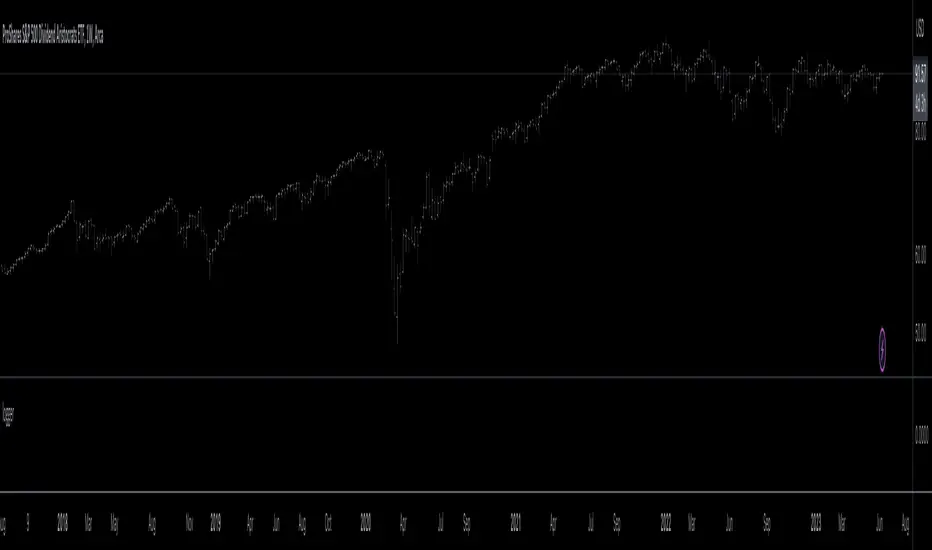
Chatterjee CorrelationThis is my first attempt on implementing a statistical method. This problem was given to me by @lejmer (who also helped me later on building more efficient code to achieve this) when we were debating on the need for higher resource allocation to run scripts so it can run longer and faster. The major problem faced by those who want to implement statistics based methods is that they run out of processing time or need to limit the data samples. My point was that such things need be implemented with an algorithm which suits pine instead of trying to port a python code directly. And yes, I am able to demonstrate that by using this implementation of Chatterjee Correlation.
🎲 What is Chatterjee Correlation?
The Chatterjee rank Correlation Coefficient (CCC) is a method developed by Sourav Chatterjee which can be used to study non linear correlation between two series.
Full documentation on the method can be found here:
arxiv.org
In short, the formula which we are implementing here is:
Algorithm can be simplified as follows:
1. Get the ranks of X
2. Get the ranks of Y
3. Sort ranks of Y in the order of X (Lets call this SortedYIndices)
4. Calculate the sum of adjacent Y ranks in SortedYIndices (Lets call it as SumOfAdjacentSortedIndices)
5. And finally the correlation coefficient can be calculated by using simple formula
CCC = 1 - (3*SumOfAdjacentSortedIndices)/(n^2 - 1)
🎲 Looks simple? What is the catch?
Mistake many people do here is that they think in Python/Java/C etc while coding in Pine. This makes code less efficient if it involves arrays and loops. And the simple code may look something like this.
var xArray = array.new()
var yArray = array.new()
array.push(xArray, x)
array.push(yArray, y)
sortX = array.sort_indices(xArray)
sortY = array.sort_indices(yArray)
SumOfAdjacentSortedIndices = 0.0
index = array.get(xSortIndices, 0)
for i=1 to n > 1? n -1 : na
indexNext = array.get(sortX, i)
SumOfAdjacentSortedIndices += math.abs(array.get(sortY, indexNext)-array.get(sortY, index))
index := indexNext
correlation := 1 - 3*SumOfAdjacentSortedIndices/(math.pow(n,2)-1)
But, problem here is the number of loops run. Remember pine executes the code on every bar. There are loops run in array.sort_indices and another loop we are running to calculate SumOfAdjacentSortedIndices. Due to this, chances of program throwing runtime errors due to script running for too long are pretty high. This limits greatly the number of samples against which we can run the study. The options to overcome are
Limit the sample size and calculate only between certain bars - this is not ideal as smaller sets are more likely to yield false or inconsistent results.
Start thinking in pine instead of python and code in such a way that it is optimised for pine. - This is exactly what we have done in the published code.
🎲 How to think in Pine?
In order to think in pine, you should try to eliminate the loops as much as possible. Specially on the data which is continuously growing.
My first thought was that sorting takes lots of time and need to find a better way to sort series - specially when it is a growing data set. Hence, I came up with this library which implements Binary Insertion Sort.
Replacing array.sort_indices with binary insertion sort will greatly reduce the number of loops run on each bar. In binary insertion sort, the array will remain sorted and any item we add, it will keep adding it in the existing sort order so that there is no need to run separate sort. This allows us to work with bigger data sets and can utilise full 20,000 bars for calculation instead of few 100s.
However, last loop where we calculate SumOfAdjacentSortedIndices is not replaceable easily. Hence, we only limit these iterations to certain bars (Even though we use complete sample size). Plots are made for only those bars where the results need to be printed.
🎲 Implementation
Current implementation is limited to few combinations of x and fixed y. But, will be converting this into library soon - which means, programmers can plug any x and y and get the correlation.
Our X here can be
Average volume
ATR
And our Y is distance of price from moving average - which identifies trend.
Thus, the indicator here helps to understand the correlation coefficient between volume and trend OR volatility and trend for given ticker and timeframe. Value closer to 1 means highly correlated and value closer to 0 means least correlated. Please note that this method will not tell how these values are correlated. That is, we will not be able to know if higher volume leads to higher trend or lower trend. But, we can say whether volume impacts trend or not.
Please note that values can differ by great extent for different timeframes. For example, if you look at 1D timeframe, you may get higher value of correlation coefficient whereas lower value for 1m timeframe. This means, volume to trend correlation is higher in 1D timeframe and lower in lower timeframes.

FrizBugLibrary "FrizBug"
Debug Tools | Pinescript Debugging Tool Kit
All in one Debugger - the benefit of wrapper functions to simply wrap variables or outputs and have the code still execute the same. Perfect for Debugging on Pine
str(inp)
Overloaded tostring like Function for all type+including Object Variables will also do arrays and matricies of all Types
Parameters:
inp : All types
Returns: string
print_label(str, x_offset, y, barstate, style, color, textcolor, text_align, size)
Label Helper Function - only needs the Str input to work
Parameters:
str :
x_offset : offset from last bar + or -
y : price of label
barstate : barstate built in variable
style : label style settin7
color : color setting
textcolor : textcolor
text_align : text align setting
size : text_sise
Returns: label
init()
initializes the database arrays
Returns: tuple | 2 matrix (1 matrix is varip(live) the other is reagular var (Bar))
update(log, live, live_console, log_console, live_lbl, log_lbl)
Put at the very end of your code / This updates all of the consoles
Parameters:
log : This matrix is the one used for Bar updates
live : This matrix is the one used for Real Time updates
live_console : on_offs for the consoles and lbls - call in the update function
log_console : on_offs for the consoles and lbls - call in the update function
live_lbl : on_offs for the consoles and lbls - call in the update function
log_lbl : on_offs for the consoles and lbls - call in the update function
Returns: void
log(log, inp, str_label, off, rows, index_cols, bars_back)
Function Will push to the Console offset to the right of Current bar, This is the main Console - it has 2 Feeds left and right (changeable)"
Parameters:
log : Matrix - Log or Live
inp : All types
str_label : (optional) This input will label it on the feed
off : Useful for when you don't want to remove the function"
rows : when printing or logging a matrix this will shorten the output will show last # of rows"
index_cols : When printing or logging a array or matrix this will shorten the array or the columns of a matrix by the #"
bars_back : Adjustment for Bars Back - Default is 1 (0 for barstate.islast)"
Returns: inp - all types (The log and print functions can be used as wrapper functions see usage below for examples)
Print(log, str_label, off, bars_back)
Function can be used to send information to a label style Console, Can be used as a wrapper function, Similar to str.format use with str()
Parameters:
log :
str_label : (optional) Can be used to label Data sent to the Console
off : Useful for when you don't want to remove the function
bars_back : Adjustment for Bars Back - Default is 1 (0 for barstate.islast)
Returns: string
print(inp, str_label, off, bars_back)
This Function can be used to send information to a label style Console, Can be used as a wrapper function, Overload print function
Parameters:
inp : All types
str_label : string (optional) Can be used to label Data sent to the Console
off : Useful for when you don't want to remove the function
bars_back : Adjustment for Bars Back - Default is 1 (0 for barstate.islast)
Returns: inp - all types (The log and print functions can be used as wrapper functions see usage below for examples)
Credits:
@kaigouthro - for the font library
@RicardoSantos - for the concept I used to make this
Thanks!
Use cases at the bottom
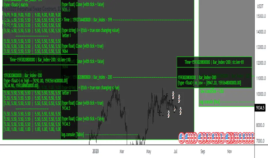
chart visible bar timeWith the latest added features chart.left_visible_bar_time and chart.right_visible_bar_time it is now possible to
place label.new() positions at the equivalent of 'location.top' and 'location.bottom'
The following are examples of functions which enables to find the visible chart highest/lowest bars:
highest_visible_chart() =>
var float highs = na
highs := time == chart.left_visible_bar_time ? high :
time > chart.left_visible_bar_time and high > highs ? high : highs
lowest_visible_chart() =>
var float lows = na
lows := time == chart.left_visible_bar_time ? low :
time > chart.left_visible_bar_time and low < lows ? low : lows
In this example labels are plotted when a sma crosses another sma
Also combined with 3 boxes, scrolling gives insights how the features work
To all who make Tradingview the way it is, lots and lots of thanks!
Cheers!

LutrewMTF// ————— Plots
var cMarkerUp = color.new(color.lime, 0)
var cMarkerDn = color.new(color.red, 0)
plotshape(A1U, "Marker 1 Up", shape.triangleup, location.belowbar, cMarkerUp, size = size.tiny, text = "1")
plotshape(A2D, "Marker 2 Dn", shape.triangledown, location.abovebar, cMarkerDn, size = size.tiny, text = "2")
plotshape(A3U, "Marker 3 Up", shape.triangleup, location.belowbar, cMarkerUp, size = size.tiny, text = "\n3")
plotshape(A4D, "Marker 4 Dn", shape.triangledown, location.abovebar, cMarkerDn, size = size.tiny, text = "4\n")
plotshape(A5U, "Marker 5 Up", shape.triangleup, location.belowbar, cMarkerUp, size = size.tiny, text = "\n\n5")
plotshape(A6D, "Marker 6 Dn", shape.triangledown, location.abovebar, cMarkerDn, size = size.tiny, text = "6\n\n")
plotshape(A7U, "Marker 7 Up", shape.triangleup, location.belowbar, cMarkerUp, size = size.tiny, text = "\n\n7")
plotshape(A8D, "Marker 8 Dn", shape.triangledown, location.abovebar, cMarkerDn, size = size.tiny, text = "8\n\n")
// ————— Alert
alertcondition( A1U or A2D or A3U or A4D or A5U or A6D or A7U or A8D, "Pivots MTF: Configured Markers", "Pivots MTF Alert")
// }
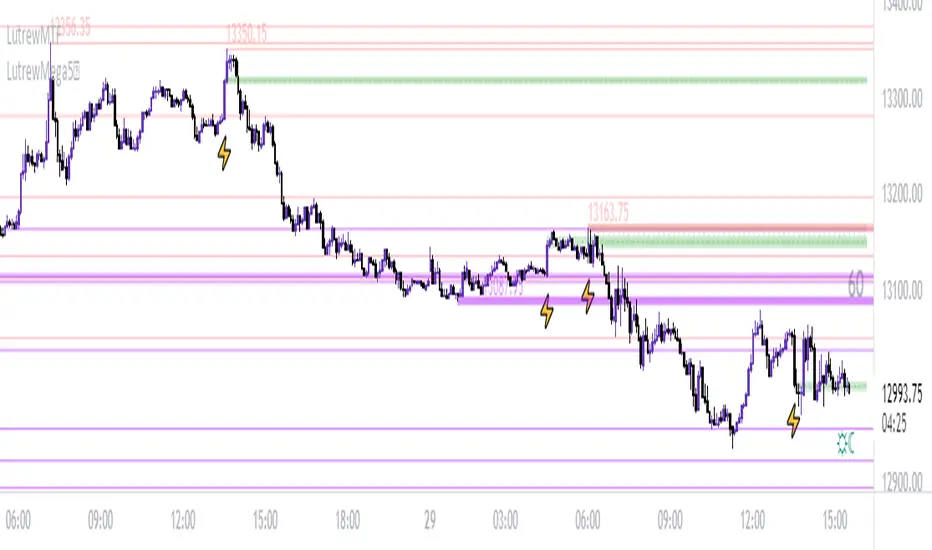
HOTT and LOTTA brand new indicator adaptation via ott from OTT developer Anıl Özekşi.
Optimized Trend Tracker, OTT is an indicator that provides traders to find an existing trend or in another words to ser which side of the current trend we are on. Kıvanç Özbilgiç coded OTT from the matrix program and adapted it to tradingview.
This indicator adaptation works with patch logic. Ott is created with the support of 10 bars Highest High and Lowest Low. The settings that the creator uses are the standard existing settings.
Here is the HighestOTT (HOTT) Line,
In general, what you need to see here is that prices tend to touch prices as they go up.
If the prices are rising, it tries to go below them, if it cannot, at least it tries to move within it.
When the price is flat or falling, it stays above the prices without touching them. This shows that our patch can do its job, which we wanted at the beginning, to protect us from horizontals and falls during purchase.
Here is the LowestOTT (LOTT) Line,
As you can notice, it uses similar construction as a structure. The only difference is that what we just did with Highest High, we are now trying to bring out the opposite effect by doing it with Lowest Low.
Now let's see hott and lott together. The places I want to draw your attention to are that prices are always above LOTT where they are on the up and sideways, and below HOTT when they are on the downtrend.
In this case, you must have understood the working principles of our patches.
If the prices are above the blue line, that is, HOTT, our buying door is opened, and as long as it is below, the buying door will remain closed.
Likewise, if the prices are below the purple line, that is, LOTT, our sales door is opened, and as long as it is above the sales door will remain closed.
Bar colors are also designed accordingly.
There is an Extra Plot Candle option in the settings tab of the indicator. This option is designed so that you can use bar colors efficiently while using normal candles. In order to use this option properly, you need to turn off the candle, border and wick colors in the symbol section of the graphic settings.
Built in Moving Average type defaultly set as VAR but users can choose from 8 different Moving Average types like:
SMA : Simple Moving Average
EMA : Exponential Moving Average
WMA : Weighted Moving Average
TMA : Triangular Moving Average
VAR : Variable Index Dynamic Moving Average a.k.a. VIDYA
WWMA : Welles Wilder's Moving Average
ZLEMA : Zero Lag Exponential Moving Average
TSF : True Strength Force
Best regards to Anıl Özekşi and Kıvanç Özbilgiç.
