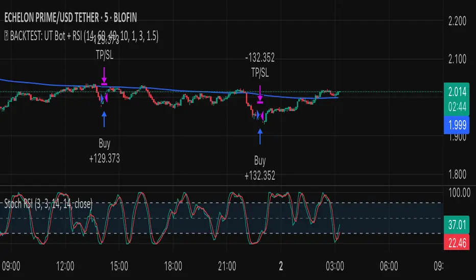
Поиск скриптов по запросу "backtest"
Moving Averages Cross - MTF - StrategyBacktesting Script for the following strategy
Strategy Injector Source: github.com
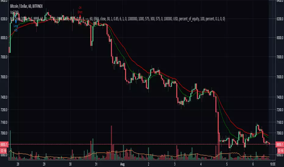
4H CCI Strategy 1.5Included adaptive lot size based on ATR, and also ATR based stop and take profit levels.
Risk/reward increased to 1:2 and should work in all ranging FX pairs as long as they are not trending.
Once the market starts trending it'll eat this bot alive.
Cheers,
Ivan Labrie
Time at Mode FX
[SM-021-v1.1] Gaussian Channel Strategy - Long & ShortThis is a trend-following breakout strategy that combines a sophisticated Moving Average (the Gaussian Channel) with a momentum oscillator (Stochastic RSI).
It aims to catch strong trend moves when the price breaks outside of the volatility bands, using the Stochastic RSI to confirm sufficient momentum exists.
Here is a detailed breakdown of how the strategy works:
1. Primary Indicator: The Gaussian Channel
The core of this strategy is a custom indicator originally developed by DonovanWall. It is designed to reduce the "lag" (delay) typically found in standard moving averages while remaining very smooth.
The Filter (Middle Line): It calculates a "Pole" based Gaussian filter. If the line is sloping up, it paints green (bullish); if sloping down, it paints red (bearish).
The Bands (Volatility): It calculates a True Range (volatility) multiplier to create an Upper Band (hband) and a Lower Band (lband).
Lag Reduction: The script includes logic to artificially reduce lag or increase response speed (modeLag and modeFast inputs).
2. Secondary Indicator: Stochastic RSI
The strategy uses standard Stochastic RSI settings (14, 100, 3, 3 inputs) to measure momentum.
K Line: The primary line used for decision-making in this script.
3. Strategy Logic
Long Trade Setup (Buying)
The strategy enters a Long position when ALL of the following conditions are met:
Trend is Bullish: The Gaussian Filter is sloping upwards (Green).
Breakout: The Closing Price is above the Gaussian Upper Band (hband).
Momentum Validation: The Stoch RSI k line is at an extreme reading (either > 80 or < 20). This implies the script looks for high volatility/momentum, regardless of whether it is traditionally "overbought" or "oversold."
Date & Toggle: The current date is within the backtesting range, and "Enable Long Trading" is turned on.
Long Exit (Selling)
The strategy closes the Long position when the Price crosses under the Gaussian Upper Band.
Interpretation: It rides the breakout wave, but as soon as price weakens and falls back inside the volatility channel, the trade is closed.
Short Trade Setup (Selling)
The strategy enters a Short position when ALL of the following conditions are met:
Trend is Bearish: The Gaussian Filter is sloping downwards (Red).
Breakout: The Closing Price is below the Gaussian Lower Band (lband).
Momentum Validation: The Stoch RSI k line is at an extreme reading (either > 80 or < 20).
Date & Toggle: The current date is within the backtesting range, and "Enable Short Trading" is turned on.
Short Exit (Covering)
The strategy closes the Short position when the Price crosses over the Gaussian Lower Band.
4. Visuals & Settings
Chart Overlay: The bands and the middle line are plotted on the chart.
Bar Colors: The candlesticks change color based on their position relative to the bands and the previous candle (e.g., bright green for strong bullish breakouts, bright red for strong bearish breakouts).
Backtesting Inputs:
Capital: Starts with $1,000.
Position Size: Uses 100% of equity per trade.
Date Range: Filters trades between 2018 and 2069.
Summary
This is a momentum breakout strategy . It does not try to buy the bottom or sell the top. Instead, it waits for the trend to establish itself (Gaussian slope) and for the price to explode outside of normal volatility ranges (Bands). It uses the Stoch RSI to ensure the move has enough "juice" behind it, and it exits quickly if the price retreats back into the normal range.
Hash Ratings EngineHash Ratings Engine - Technical Consensus Strategy
A systematic trading strategy that harnesses TradingView's Technical Ratings to generate high-conviction entries with institutional-grade risk management.
What It Does
This strategy aggregates the consensus of 26+ technical indicators (RSI, MACD, Stochastics, multiple Moving Averages, etc.) into a single actionable signal. When enough indicators align bullish or bearish, the engine triggers an entry. Built-in trend filtering and ATR-based exits keep you on the right side of the market.
Key Features
Trend Filter - Only takes longs in uptrends, shorts in downtrends. This single filter typically improves results by 20-40% by avoiding counter-trend trades.
ATR-Based Risk Management - Stop loss and trailing stops adapt to current market volatility. Tight stops in calm markets, wider stops in volatile conditions.
Cooldown System - After a losing trade, the strategy waits before re-entering. This prevents the consecutive loss streaks that destroy accounts.
Clean Visuals - Fluorescent entry/exit signals with price level references. See exactly where you got in and out.
Settings Guide
Indicator Timeframe: Leave blank for current chart. Use higher timeframe for fewer, higher-quality signals.
Rating Source: "All" for balanced approach. "MAs" for trend-following. "Oscillators" for mean-reversion.
Entry Thresholds
Strong Signal Threshold: Higher = fewer trades but better conviction. Start at 0.5, test 0.4-0.6.
Risk Management
ATR Period: 12 is responsive, 14 is standard, 20+ is smoother.
Stop Loss: 2-3x ATR for tight stops, 3.5-4x for moderate, 5x+ for wide.
Trail Activation: How far price must move in profit before trailing begins.
Trail Offset: How closely the trail follows price.
Trend Filter
EMA Length: 150 works well on 4H charts. Use 100 for lower timeframes, 200 for daily.
Trade Timing
Cooldown: Keep enabled. 5 bars is a good starting point.
Best Practices
Start with default settings and backtest on your preferred instrument. Adjust the Strong Signal Threshold first - this has the biggest impact on trade frequency. Then tune the EMA length to match your timeframe. Finally, optimize the ATR multipliers for your risk tolerance.
Works on any liquid market - crypto, forex, stocks, futures. Higher timeframes (4H, Daily) tend to produce cleaner signals than lower timeframes.
Disclaimer
Past performance does not guarantee future results. Always backtest thoroughly and use proper position sizing. This strategy is for educational purposes - trade at your own risk.
Asset Rotation System [InvestorUnknown]Overview
This system creates a comprehensive trend "matrix" by analyzing the performance of six assets against both the US Dollar and each other. The objective is to identify and hold the asset that is currently outperforming all others, thereby focusing on maintaining an investment in the most "optimal" asset at any given time.
- - - Key Features - - -
1. Trend Classification:
The system evaluates the trend for each of the six assets, both individually against USD and in pairs (assetX/assetY), to determine which asset is currently outperforming others.
Utilizes five distinct trend indicators: RSI (50 crossover), CCI, SuperTrend, DMI, and Parabolic SAR.
Users can customize the trend analysis by selecting all indicators or choosing a single one via the "Trend Classification Method" input setting.
2. Backtesting:
Calculates an equity curve for each asset and for the system itself, which assumes holding only the asset deemed optimal at any time.
Customizable start date for backtesting; by default, it begins either 5000 bars ago (the maximum in TradingView) or at the inception of the youngest asset included, whichever is shorter. If the youngest asset's history exceeds 5000 bars, the system uses 5000 bars to prevent errors.
The equity curve is dynamically colored based on the asset held at each point, with this coloring also reflected on the chart via barcolor().
Performance metrics like returns, standard deviation of returns, Sharpe, Sortino, and Omega ratios, along with maximum drawdown, are computed for each asset and the system's equity curve.
3 Alerts:
Supports alerts for when a new, confirmed optimal asset is identified. However, due to TradingView limitations, the specific asset cannot be included in the alert message.
- - - Usage - - -
1. Select Assets/Tickers:
Choose which assets or tickers you want to include in the rotation system. Ensure that all selected tickers are denominated in USD to maintain consistency in analysis.
2. Configure Trend Classification:
Decide on the trend classification method from the available options (RSI, CCI, SuperTrend, DMI, or Parabolic SAR, All) and adjust the settings to your preferences. This customization allows you to tailor the system to different market conditions or your specific trading strategy.
3. Utilize Backtesting for Calibration:
Use the backtesting results, including equity curves and performance metrics, to fine-tune your chosen trend indicators.
Be cautious not to overemphasize performance maximization, as this can lead to overfitting. The goal is to achieve a robust system that performs well across various market conditions, rather than just optimizing for past data.
- - - Parameters - - -
Tickers:
Asset 1: Select the symbol for the first asset.
Asset 2: Select the symbol for the second asset.
Asset 3: Select the symbol for the third asset.
Asset 4: Select the symbol for the fourth asset.
Asset 5: Select the symbol for the fifth asset.
Asset 6: Select the symbol for the sixth asset.
General Settings:
Trend Classification Method: Choose from RSI, CCI, SuperTrend, DMI, PSAR, or "All" to determine how trends are analyzed.
Use Custom Starting Date for Backtest: Toggle to use a custom date for beginning the backtest.
Custom Starting Date: Set the custom start date for backtesting.
Plot Perf. Metrics Table: Option to display performance metrics in a table on the chart.
RSI (Relative Strength Index):
RSI Source: Choose the price data source for RSI calculation.
RSI Length: Set the period for the RSI calculation.
CCI (Commodity Channel Index):
CCI Source: Select the price data source for CCI calculation.
CCI Length: Determine the period for the CCI.
SuperTrend:
SuperTrend Factor: Adjust the sensitivity of the SuperTrend indicator.
SuperTrend Length: Set the period for the SuperTrend calculation.
DMI (Directional Movement Index):
DMI Length: Define the period for DMI calculations.
Parabolic SAR:
PSAR Start: Initial acceleration factor for the Parabolic SAR.
PSAR Increment: Increment value for the acceleration factor.
PSAR Max Value: Maximum value the acceleration factor can reach.
Notes/Recommendations:
While this system is operational, it's important to recognize that it relies on "basic" indicators, which may not be ideal for generating trading signals on their own. I strongly suggest that users delve into the code to grasp the underlying logic of the system. Consider customizing it by integrating more sophisticated and higher-quality trend-following indicators to enhance its performance and reliability.
Disclaimer:
This system's backtest results are historical and do not predict future performance. Use for educational purposes only; not investment advice.
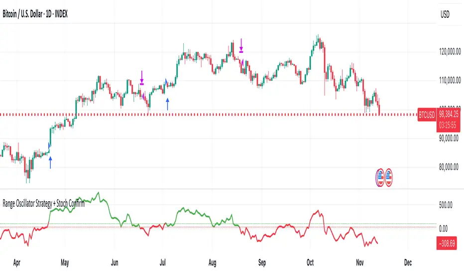
Range Oscillator Strategy + Stoch Confirm🔹 Short summary
This is a free, educational long-only strategy built on top of the public “Range Oscillator” by Zeiierman (used under CC BY-NC-SA 4.0), combined with a Stochastic timing filter, an EMA-based exit filter and an optional risk-management layer (SL/TP and R-multiple exits). It is NOT financial advice and it is NOT a magic money machine. It’s a structured framework to study how range-expansion + momentum + trend slope can be combined into one rule-based system, often with intentionally RARE trades.
────────────────────────
0. Legal / risk disclaimer
────────────────────────
• This script is FREE and public. I do not charge any fee for it.
• It is for EDUCATIONAL PURPOSES ONLY.
• It is NOT financial advice and does NOT guarantee profits.
• Backtest results can be very different from live results.
• Markets change over time; past performance is NOT indicative of future performance.
• You are fully responsible for your own trades and risk.
Please DO NOT use this script with money you cannot afford to lose. Always start in a demo / paper trading environment and make sure you understand what the logic does before you risk any capital.
────────────────────────
1. About default settings and risk (very important)
────────────────────────
The script is configured with the following defaults in the `strategy()` declaration:
• `initial_capital = 10000`
→ This is only an EXAMPLE account size.
• `default_qty_type = strategy.percent_of_equity`
• `default_qty_value = 100`
→ This means 100% of equity per trade in the default properties.
→ This is AGGRESSIVE and should be treated as a STRESS TEST of the logic, not as a realistic way to trade.
TradingView’s House Rules recommend risking only a small part of equity per trade (often 1–2%, max 5–10% in most cases). To align with these recommendations and to get more realistic backtest results, I STRONGLY RECOMMEND you to:
1. Open **Strategy Settings → Properties**.
2. Set:
• Order size: **Percent of equity**
• Order size (percent): e.g. **1–2%** per trade
3. Make sure **commission** and **slippage** match your own broker conditions.
• By default this script uses `commission_value = 0.1` (0.1%) and `slippage = 3`, which are reasonable example values for many crypto markets.
If you choose to run the strategy with 100% of equity per trade, please treat it ONLY as a stress-test of the logic. It is NOT a sustainable risk model for live trading.
────────────────────────
2. What this strategy tries to do (conceptual overview)
────────────────────────
This is a LONG-ONLY strategy designed to explore the combination of:
1. **Range Oscillator (Zeiierman-based)**
- Measures how far price has moved away from an adaptive mean.
- Uses an ATR-based range to normalize deviation.
- High positive oscillator values indicate strong price expansion away from the mean in a bullish direction.
2. **Stochastic as a timing filter**
- A classic Stochastic (%K and %D) is used.
- The logic requires %K to be below a user-defined level and then crossing above %D.
- This is intended to catch moments when momentum turns up again, rather than chasing every extreme.
3. **EMA Exit Filter (trend slope)**
- An EMA with configurable length (default 70) is calculated.
- The slope of the EMA is monitored: when the slope turns negative while in a long position, and the filter is enabled, it triggers an exit condition.
- This acts as a trend-protection exit: if the medium-term trend starts to weaken, the strategy exits even if the oscillator has not yet fully reverted.
4. **Optional risk-management layer**
- Percentage-based Stop Loss and Take Profit (SL/TP).
- Risk/Reward (R-multiple) exit based on the distance from entry to SL.
- Implemented as OCO orders that work *on top* of the logical exits.
The goal is not to create a “holy grail” system but to serve as a transparent, configurable framework for studying how these concepts behave together on different markets and timeframes.
────────────────────────
3. Components and how they work together
────────────────────────
(1) Range Oscillator (based on “Range Oscillator (Zeiierman)”)
• The script computes a weighted mean price and then measures how far price deviates from that mean.
• Deviation is normalized by an ATR-based range and expressed as an oscillator.
• When the oscillator is above the **entry threshold** (default 100), it signals a strong move away from the mean in the bullish direction.
• When it later drops below the **exit threshold** (default 30), it can trigger an exit (if enabled).
(2) Stochastic confirmation
• Classic Stochastic (%K and %D) is calculated.
• An entry requires:
- %K to be below a user-defined “Cross Level”, and
- then %K to cross above %D.
• This is a momentum confirmation: the strategy tries to enter when momentum turns up from a pullback rather than at any random point.
(3) EMA Exit Filter
• The EMA length is configurable via `emaLength` (default 70).
• The script monitors the EMA slope: it computes the relative change between the current EMA and the previous EMA.
• If the slope turns negative while the strategy holds a long position and the filter is enabled, it triggers an exit condition.
• This is meant to help protect profits or cut losses when the medium-term trend starts to roll over, even if the oscillator conditions are not (yet) signalling exit.
(4) Risk management (optional)
• Stop Loss (SL) and Take Profit (TP):
- Defined as percentages relative to average entry price.
- Both are disabled by default, but you can enable them in the Inputs.
• Risk/Reward Exit:
- Uses the distance from entry to SL to project a profit target at a configurable R-multiple.
- Also optional and disabled by default.
These exits are implemented as `strategy.exit()` OCO orders and can close trades independently of oscillator/EMA conditions if hit first.
────────────────────────
4. Entry & Exit logic (high level)
────────────────────────
A) Time filter
• You can choose a **Start Year** in the Inputs.
• Only candles between the selected start date and 31 Dec 2069 are used for backtesting (`timeCondition`).
• This prevents accidental use of tiny cherry-picked windows and makes tests more honest.
B) Entry condition (long-only)
A long entry is allowed when ALL the following are true:
1. `timeCondition` is true (inside the backtest window).
2. If `useOscEntry` is true:
- Range Oscillator value must be above `entryLevel`.
3. If `useStochEntry` is true:
- Stochastic condition (`stochCondition`) must be true:
- %K < `crossLevel`, then %K crosses above %D.
If these filters agree, the strategy calls `strategy.entry("Long", strategy.long)`.
C) Exit condition (logical exits)
A position can be closed when:
1. `timeCondition` is true AND a long position is open, AND
2. At least one of the following is true:
- If `useOscExit` is true: Oscillator is below `exitLevel`.
- If `useMagicExit` (EMA Exit Filter) is true: EMA slope is negative (`isDown = true`).
In that case, `strategy.close("Long")` is called.
D) Risk-management exits
While a position is open:
• If SL or TP is enabled:
- `strategy.exit("Long Risk", ...)` places an OCO stop/limit order based on the SL/TP percentages.
• If Risk/Reward exit is enabled:
- `strategy.exit("RR Exit", ...)` places an OCO order using a projected R-multiple (`rrMult`) of the SL distance.
These risk-based exits can trigger before the logical oscillator/EMA exits if price hits those levels.
────────────────────────
5. Recommended backtest configuration (to avoid misleading results)
────────────────────────
To align with TradingView House Rules and avoid misleading backtests:
1. **Initial capital**
- 10 000 (or any value you personally want to work with).
2. **Order size**
- Type: **Percent of equity**
- Size: **1–2%** per trade is a reasonable starting point.
- Avoid risking more than 5–10% per trade if you want results that could be sustainable in practice.
3. **Commission & slippage**
- Commission: around 0.1% if that matches your broker.
- Slippage: a few ticks (e.g. 3) to account for real fills.
4. **Timeframe & markets**
- Volatile symbols (e.g. crypto like BTCUSDT, or major indices).
- Timeframes: 1H / 4H / **1D (Daily)** are typical starting points.
- I strongly recommend trying the strategy on **different timeframes**, for example 1D, to see how the behaviour changes between intraday and higher timeframes.
5. **No “caution warning”**
- Make sure your chosen symbol + timeframe + settings do not trigger TradingView’s caution messages.
- If you see warnings (e.g. “too few trades”), adjust timeframe/symbol or the backtest period.
────────────────────────
5a. About low trade count and rare signals
────────────────────────
This strategy is intentionally designed to trade RARELY:
• It is **long-only**.
• It uses strict filters (Range Oscillator threshold + Stochastic confirmation + optional EMA Exit Filter).
• On higher timeframes (especially **1D / Daily**) this can result in a **low total number of trades**, sometimes WELL BELOW 100 trades over the whole backtest.
TradingView’s House Rules mention 100+ trades as a guideline for more robust statistics. In this specific case:
• The **low trade count is a conscious design choice**, not an attempt to cherry-pick a tiny, ultra-profitable window.
• The goal is to study a **small number of high-conviction long entries** on higher timeframes, not to generate frequent intraday signals.
• Because of the low trade count, results should NOT be interpreted as statistically strong or “proven” – they are only one sample of how this logic would have behaved on past data.
Please keep this in mind when you look at the equity curve and performance metrics. A beautiful curve with only a handful of trades is still just a small sample.
────────────────────────
6. How to use this strategy (step-by-step)
────────────────────────
1. Add the script to your chart.
2. Open the **Inputs** tab:
- Set the backtest start year.
- Decide whether to use Oscillator-based entry/exit, Stochastic confirmation, and EMA Exit Filter.
- Optionally enable SL, TP, and Risk/Reward exits.
3. Open the **Properties** tab:
- Set a realistic account size if you want.
- Set order size to a realistic % of equity (e.g. 1–2%).
- Confirm that commission and slippage are realistic for your broker.
4. Run the backtest:
- Look at Net Profit, Max Drawdown, number of trades, and equity curve.
- Remember that a low trade count means the statistics are not very strong.
5. Experiment:
- Tweak thresholds (`entryLevel`, `exitLevel`), Stochastic settings, EMA length, and risk params.
- See how the metrics and trade frequency change.
6. Forward-test:
- Before using any idea in live trading, forward-test on a demo account and observe behaviour in real time.
────────────────────────
7. Originality and usefulness (why this is more than a mashup)
────────────────────────
This script is not intended to be a random visual mashup of indicators. It is designed as a coherent, testable strategy with clear roles for each component:
• Range Oscillator:
- Handles mean vs. range-expansion states via an adaptive, ATR-normalized metric.
• Stochastic:
- Acts as a timing filter to avoid entering purely on extremes and instead waits for momentum to turn.
• EMA Exit Filter:
- Trend-slope-based safety net to exit when the medium-term direction changes against the position.
• Risk module:
- Provides practical, rule-based exits: SL, TP, and R-multiple exit, which are useful for structuring risk even if you modify the core logic.
It aims to give traders a ready-made **framework to study and modify**, not a black box or “signals” product.
────────────────────────
8. Limitations and good practices
────────────────────────
• No single strategy works on all markets or in all regimes.
• This script is long-only; it does not short the market.
• Performance can degrade when market structure changes.
• Overfitting (curve fitting) is a real risk if you endlessly tweak parameters to maximise historical profit.
Good practices:
- Test on multiple symbols and timeframes.
- Focus on stability and drawdown, not only on how high the profit line goes.
- View this as a learning tool and a basis for your own research.
────────────────────────
9. Licensing and credits
────────────────────────
• Core oscillator idea & base code:
- “Range Oscillator (Zeiierman)”
- © Zeiierman, licensed under CC BY-NC-SA 4.0.
• Strategy logic, Stochastic confirmation, EMA Exit Filter, and risk-management layer:
- Modifications by jokiniemi.
Please respect both the original license and TradingView House Rules if you fork or republish any part of this script.
────────────────────────
10. No payments / no vendor pitch
────────────────────────
• This script is completely FREE to use on TradingView.
• There is no paid subscription, no external payment link, and no private signals group attached to it.
• If you have questions, please use TradingView’s comment system or private messages instead of expecting financial advice.
Use this script as a tool to learn, experiment, and build your own understanding of markets.
────────────────────────
11. Example backtest settings used in screenshots
────────────────────────
To avoid any confusion about how the results shown in screenshots were produced, here is one concrete example configuration:
• Symbol: BTCUSDT (or similar major BTC pair)
• Timeframe: 1D (Daily)
• Backtest period: from 2018 to the most recent data
• Initial capital: 10 000
• Order size type: Percent of equity
• Order size: 2% per trade
• Commission: 0.1%
• Slippage: 3 ticks
• Risk settings: Stop Loss and Take Profit disabled by default, Risk/Reward exit disabled by default
• Filters: Range Oscillator entry/exit enabled, Stochastic confirmation enabled, EMA Exit Filter enabled
If you change any of these settings (symbol, timeframe, risk per trade, commission, slippage, filters, etc.), your results will look different. Please always adapt the configuration to your own risk tolerance, market, and trading style.
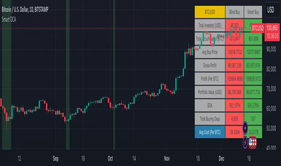
Smart DCA Strategy (Public)INSPIRATION
While Dollar Cost Averaging (DCA) is a popular and stress-free investment approach, I noticed an opportunity for enhancement. Standard DCA involves buying consistently, regardless of market conditions, which can sometimes mean missing out on optimal investment opportunities. This led me to develop the Smart DCA Strategy – a 'set and forget' method like traditional DCA, but with an intelligent twist to boost its effectiveness.
The goal was to build something more profitable than a standard DCA strategy so it was equally important that this indicator could backtest its own results in an A/B test manner against the regular DCA strategy.
WHY IS IT SMART?
The key to this strategy is its dynamic approach: buying aggressively when the market shows signs of being oversold, and sitting on the sidelines when it's not. This approach aims to optimize entry points, enhancing the potential for better returns while maintaining the simplicity and low stress of DCA.
WHAT THIS STRATEGY IS, AND IS NOT
This is an investment style strategy. It is designed to improve upon the common standard DCA investment strategy. It is therefore NOT a day trading strategy. Feel free to experiment with various timeframes, but it was designed to be used on a daily timeframe and that's how I recommend it to be used.
You may also go months without any buy signals during bull markets, but remember that is exactly the point of the strategy - to keep your buying power on the sidelines until the markets have significantly pulled back. You need to be patient and trust in the historical backtesting you have performed.
HOW IT WORKS
The Smart DCA Strategy leverages a creative approach to using Moving Averages to identify the most opportune moments to buy. A trigger occurs when a daily candle, in its entirety including the high wick, closes below the threshold line or box plotted on the chart. The indicator is designed to facilitate both backtesting and live trading.
HOW TO USE
Settings:
The input parameters for tuning have been intentionally simplified in an effort to prevent users falling into the overfitting trap.
The main control is the Buying strictness scale setting. Setting this to a lower value will provide more buying days (less strict) while higher values mean less buying days (more strict). In my testing I've found level 9 to provide good all round results.
Validation days is a setting to prevent triggering entries until the asset has spent a given number of days (candles) in the overbought state. Increasing this makes entries stricter. I've found 0 to give the best results across most assets.
In the backtest settings you can also configure how much to buy for each day an entry triggers. Blind buy size is the amount you would buy every day in a standard DCA strategy. Smart buy size is the amount you would buy each day a Smart DCA entry is triggered.
You can also experiment with backtesting your strategy over different historical datasets by using the Start date and End date settings. The results table will not calculate for any trades outside what you've set in the date range settings.
Backtesting:
When backtesting you should use the results table on the top right to tune and optimise the results of your strategy. As with all backtests, be careful to avoid overfitting the parameters. It's better to have a setup which works well across many currencies and historical periods than a setup which is excellent on one dataset but bad on most others. This gives a much higher probability that it will be effective when you move to live trading.
The results table provides a clear visual representation as to which strategy, standard or smart, is more profitable for the given dataset. You will notice the columns are dynamically coloured red and green. Their colour changes based on which strategy is more profitable in the A/B style backtest - green wins, red loses. The key metrics to focus on are GOA (Gain on Account) and Avg Cost.
Live Trading:
After you've finished backtesting you can proceed with configuring your alerts for live trading.
But first, you need to estimate the amount you should buy on each Smart DCA entry. We can use the Total invested row in the results table to calculate this. Assuming we're looking to trade on
BTCUSD
Decide how much USD you would spend each day to buy BTC if you were using a standard DCA strategy. Lets say that is $5 per day
Enter that USD amount in the Blind buy size settings box
Check the Blind Buy column in the results table. If we set the backtest date range to the last 10 years, we would expect the amount spent on blind buys over 10 years to be $18,250 given $5 each day
Next we need to tweak the value of the Smart buy size parameter in setting to get it as close as we can to the Total Invested amount for Blind Buy
By following this approach it means we will invest roughly the same amount into our Smart DCA strategy as we would have into a standard DCA strategy over any given time period.
After you have calculated the Smart buy size, you can go ahead and set up alerts on Smart DCA buy triggers.
BOT AUTOMATION
In an effort to maintain the 'set and forget' stress-free benefits of a standard DCA strategy, I have set my personal Smart DCA Strategy up to be automated. The bot runs on AWS and I have a fully functional project for the bot on my GitHub account. Just reach out if you would like me to point you towards it. You can also hook this into any other 3rd party trade automation system of your choice using the pre-configured alerts within the indicator.
PLANNED FUTURE DEVELOPMENTS
Currently this is purely an accumulation strategy. It does not have any sell signals right now but I have ideas on how I will build upon it to incorporate an algorithm for selling. The strategy should gradually offload profits in bull markets which generates more USD which gives more buying power to rinse and repeat the same process in the next cycle only with a bigger starting capital. Watch this space!
MARKETS
Crypto:
This strategy has been specifically built to work on the crypto markets. It has been developed, backtested and tuned against crypto markets and I personally only run it on crypto markets to accumulate more of the coins I believe in for the long term. In the section below I will provide some backtest results from some of the top crypto assets.
Stocks:
I've found it is generally more profitable than a standard DCA strategy on the majority of stocks, however the results proved to be a lot more impressive on crypto. This is mainly due to the volatility and cycles found in crypto markets. The strategy makes its profits from capitalising on pullbacks in price. Good stocks on the other hand tend to move up and to the right with less significant pullbacks, therefore giving this strategy less opportunity to flourish.
Forex:
As this is an accumulation style investment strategy, I do not recommend that you use it to trade Forex.
For more info about this strategy including backtest results, please see the full description on the invite only version of this strategy named "Smart DCA Strategy"
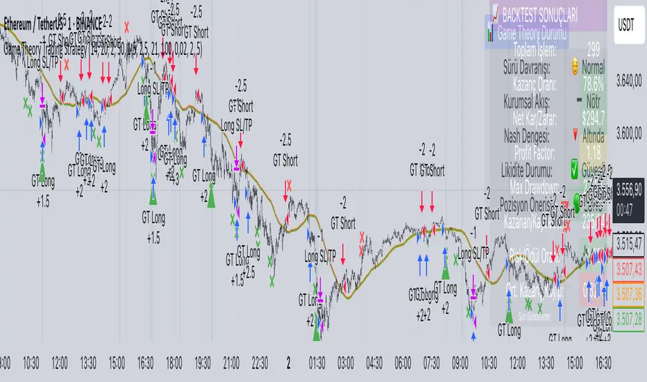
Game Theory Trading StrategyGame Theory Trading Strategy: Explanation and Working Logic
This Pine Script (version 5) code implements a trading strategy named "Game Theory Trading Strategy" in TradingView. Unlike the previous indicator, this is a full-fledged strategy with automated entry/exit rules, risk management, and backtesting capabilities. It uses Game Theory principles to analyze market behavior, focusing on herd behavior, institutional flows, liquidity traps, and Nash equilibrium to generate buy (long) and sell (short) signals. Below, I'll explain the strategy's purpose, working logic, key components, and usage tips in detail.
1. General Description
Purpose: The strategy identifies high-probability trading opportunities by combining Game Theory concepts (herd behavior, contrarian signals, Nash equilibrium) with technical analysis (RSI, volume, momentum). It aims to exploit market inefficiencies caused by retail herd behavior, institutional flows, and liquidity traps. The strategy is designed for automated trading with defined risk management (stop-loss/take-profit) and position sizing based on market conditions.
Key Features:
Herd Behavior Detection: Identifies retail panic buying/selling using RSI and volume spikes.
Liquidity Traps: Detects stop-loss hunting zones where price breaks recent highs/lows but reverses.
Institutional Flow Analysis: Tracks high-volume institutional activity via Accumulation/Distribution and volume spikes.
Nash Equilibrium: Uses statistical price bands to assess whether the market is in equilibrium or deviated (overbought/oversold).
Risk Management: Configurable stop-loss (SL) and take-profit (TP) percentages, dynamic position sizing based on Game Theory (minimax principle).
Visualization: Displays Nash bands, signals, background colors, and two tables (Game Theory status and backtest results).
Backtesting: Tracks performance metrics like win rate, profit factor, max drawdown, and Sharpe ratio.
Strategy Settings:
Initial capital: $10,000.
Pyramiding: Up to 3 positions.
Position size: 10% of equity (default_qty_value=10).
Configurable inputs for RSI, volume, liquidity, institutional flow, Nash equilibrium, and risk management.
Warning: This is a strategy, not just an indicator. It executes trades automatically in TradingView's Strategy Tester. Always backtest thoroughly and use proper risk management before live trading.
2. Working Logic (Step by Step)
The strategy processes each bar (candle) to generate signals, manage positions, and update performance metrics. Here's how it works:
a. Input Parameters
The inputs are grouped for clarity:
Herd Behavior (🐑):
RSI Period (14): For overbought/oversold detection.
Volume MA Period (20): To calculate average volume for spike detection.
Herd Threshold (2.0): Volume multiplier for detecting herd activity.
Liquidity Analysis (💧):
Liquidity Lookback (50): Bars to check for recent highs/lows.
Liquidity Sensitivity (1.5): Volume multiplier for trap detection.
Institutional Flow (🏦):
Institutional Volume Multiplier (2.5): For detecting large volume spikes.
Institutional MA Period (21): For Accumulation/Distribution smoothing.
Nash Equilibrium (⚖️):
Nash Period (100): For calculating price mean and standard deviation.
Nash Deviation (0.02): Multiplier for equilibrium bands.
Risk Management (🛡️):
Use Stop-Loss (true): Enables SL at 2% below/above entry price.
Use Take-Profit (true): Enables TP at 5% above/below entry price.
b. Herd Behavior Detection
RSI (14): Checks for extreme conditions:
Overbought: RSI > 70 (potential herd buying).
Oversold: RSI < 30 (potential herd selling).
Volume Spike: Volume > SMA(20) x 2.0 (herd_threshold).
Momentum: Price change over 10 bars (close - close ) compared to its SMA(20).
Herd Signals:
Herd Buying: RSI > 70 + volume spike + positive momentum = Retail buying frenzy (red background).
Herd Selling: RSI < 30 + volume spike + negative momentum = Retail selling panic (green background).
c. Liquidity Trap Detection
Recent Highs/Lows: Calculated over 50 bars (liquidity_lookback).
Psychological Levels: Nearest round numbers (e.g., $100, $110) as potential stop-loss zones.
Trap Conditions:
Up Trap: Price breaks recent high, closes below it, with a volume spike (volume > SMA x 1.5).
Down Trap: Price breaks recent low, closes above it, with a volume spike.
Visualization: Traps are marked with small red/green crosses above/below bars.
d. Institutional Flow Analysis
Volume Check: Volume > SMA(20) x 2.5 (inst_volume_mult) = Institutional activity.
Accumulation/Distribution (AD):
Formula: ((close - low) - (high - close)) / (high - low) * volume, cumulated over time.
Smoothed with SMA(21) (inst_ma_length).
Accumulation: AD > MA + high volume = Institutions buying.
Distribution: AD < MA + high volume = Institutions selling.
Smart Money Index: (close - open) / (high - low) * volume, smoothed with SMA(20). Positive = Smart money buying.
e. Nash Equilibrium
Calculation:
Price mean: SMA(100) (nash_period).
Standard deviation: stdev(100).
Upper Nash: Mean + StdDev x 0.02 (nash_deviation).
Lower Nash: Mean - StdDev x 0.02.
Conditions:
Near Equilibrium: Price between upper and lower Nash bands (stable market).
Above Nash: Price > upper band (overbought, sell potential).
Below Nash: Price < lower band (oversold, buy potential).
Visualization: Orange line (mean), red/green lines (upper/lower bands).
f. Game Theory Signals
The strategy generates three types of signals, combined into long/short triggers:
Contrarian Signals:
Buy: Herd selling + (accumulation or down trap) = Go against retail panic.
Sell: Herd buying + (distribution or up trap).
Momentum Signals:
Buy: Below Nash + positive smart money + no herd buying.
Sell: Above Nash + negative smart money + no herd selling.
Nash Reversion Signals:
Buy: Below Nash + rising close (close > close ) + volume > MA.
Sell: Above Nash + falling close + volume > MA.
Final Signals:
Long Signal: Contrarian buy OR momentum buy OR Nash reversion buy.
Short Signal: Contrarian sell OR momentum sell OR Nash reversion sell.
g. Position Management
Position Sizing (Minimax Principle):
Default: 1.0 (10% of equity).
In Nash equilibrium: Reduced to 0.5 (conservative).
During institutional volume: Increased to 1.5 (aggressive).
Entries:
Long: If long_signal is true and no existing long position (strategy.position_size <= 0).
Short: If short_signal is true and no existing short position (strategy.position_size >= 0).
Exits:
Stop-Loss: If use_sl=true, set at 2% below/above entry price.
Take-Profit: If use_tp=true, set at 5% above/below entry price.
Pyramiding: Up to 3 concurrent positions allowed.
h. Visualization
Nash Bands: Orange (mean), red (upper), green (lower).
Background Colors:
Herd buying: Red (90% transparency).
Herd selling: Green.
Institutional volume: Blue.
Signals:
Contrarian buy/sell: Green/red triangles below/above bars.
Liquidity traps: Red/green crosses above/below bars.
Tables:
Game Theory Table (Top-Right):
Herd Behavior: Buying frenzy, selling panic, or normal.
Institutional Flow: Accumulation, distribution, or neutral.
Nash Equilibrium: In equilibrium, above, or below.
Liquidity Status: Trap detected or safe.
Position Suggestion: Long (green), Short (red), or Wait (gray).
Backtest Table (Bottom-Right):
Total Trades: Number of closed trades.
Win Rate: Percentage of winning trades.
Net Profit/Loss: In USD, colored green/red.
Profit Factor: Gross profit / gross loss.
Max Drawdown: Peak-to-trough equity drop (%).
Win/Loss Trades: Number of winning/losing trades.
Risk/Reward Ratio: Simplified Sharpe ratio (returns / drawdown).
Avg Win/Loss Ratio: Average win per trade / average loss per trade.
Last Update: Current time.
i. Backtesting Metrics
Tracks:
Total trades, winning/losing trades.
Win rate (%).
Net profit ($).
Profit factor (gross profit / gross loss).
Max drawdown (%).
Simplified Sharpe ratio (returns / drawdown).
Average win/loss ratio.
Updates metrics on each closed trade.
Displays a label on the last bar with backtest period, total trades, win rate, and net profit.
j. Alerts
No explicit alertconditions defined, but you can add them for long_signal and short_signal (e.g., alertcondition(long_signal, "GT Long Entry", "Long Signal Detected!")).
Use TradingView's alert system with Strategy Tester outputs.
3. Usage Tips
Timeframe: Best for H1-D1 timeframes. Shorter frames (M1-M15) may produce noisy signals.
Settings:
Risk Management: Adjust sl_percent (e.g., 1% for volatile markets) and tp_percent (e.g., 3% for scalping).
Herd Threshold: Increase to 2.5 for stricter herd detection in choppy markets.
Liquidity Lookback: Reduce to 20 for faster markets (e.g., crypto).
Nash Period: Increase to 200 for longer-term analysis.
Backtesting:
Use TradingView's Strategy Tester to evaluate performance.
Check win rate (>50%), profit factor (>1.5), and max drawdown (<20%) for viability.
Test on different assets/timeframes to ensure robustness.
Live Trading:
Start with a demo account.
Combine with other indicators (e.g., EMAs, support/resistance) for confirmation.
Monitor liquidity traps and institutional flow for context.
Risk Management:
Always use SL/TP to limit losses.
Adjust position_size for risk tolerance (e.g., 5% of equity for conservative trading).
Avoid over-leveraging (pyramiding=3 can amplify risk).
Troubleshooting:
If no trades are executed, check signal conditions (e.g., lower herd_threshold or liquidity_sensitivity).
Ensure sufficient historical data for Nash and liquidity calculations.
If tables overlap, adjust position.top_right/bottom_right coordinates.
4. Key Differences from the Previous Indicator
Indicator vs. Strategy: The previous code was an indicator (VP + Game Theory Integrated Strategy) focused on visualization and alerts. This is a strategy with automated entries/exits and backtesting.
Volume Profile: Absent in this strategy, making it lighter but less focused on high-volume zones.
Wick Analysis: Not included here, unlike the previous indicator's heavy reliance on wick patterns.
Backtesting: This strategy includes detailed performance metrics and a backtest table, absent in the indicator.
Simpler Signals: Focuses on Game Theory signals (contrarian, momentum, Nash reversion) without the "Power/Ultra Power" hierarchy.
Risk Management: Explicit SL/TP and dynamic position sizing, not present in the indicator.
5. Conclusion
The "Game Theory Trading Strategy" is a sophisticated system leveraging herd behavior, institutional flows, liquidity traps, and Nash equilibrium to trade market inefficiencies. It’s designed for traders who understand Game Theory principles and want automated execution with robust risk management. However, it requires thorough backtesting and parameter optimization for specific markets (e.g., forex, crypto, stocks). The backtest table and visual aids make it easy to monitor performance, but always combine with other analysis tools and proper capital management.
If you need help with backtesting, adding alerts, or optimizing parameters, let me know!
Live Market - Performance MonitorLive Market — Performance Monitor
Study material (no code) — step-by-step training guide for learners
________________________________________
1) What this tool is — short overview
This indicator is a live market performance monitor designed for learning. It scans price, volume and volatility, detects order blocks and trendline events, applies filters (volume & ATR), generates trade signals (BUY/SELL), creates simple TP/SL trade management, and renders a compact dashboard summarizing market state, risk and performance metrics.
Use it to learn how multi-factor signals are constructed, how Greeks-style sensitivity is replaced by volatility/ATR reasoning, and how a live dashboard helps monitor trade quality.
________________________________________
2) Quick start — how a learner uses it (step-by-step)
1. Add the indicator to a chart (any ticker / timeframe).
2. Open inputs and review the main groups: Order Block, Trendline, Signal Filters, Display.
3. Start with defaults (OB periods ≈ 7, ATR multiplier 0.5, volume threshold 1.2) and observe the dashboard on the last bar.
4. Walk the chart back in time (use the last-bar update behavior) and watch how signals, order blocks, trendlines, and the performance counters change.
5. Run the hands-on labs below to build intuition.
________________________________________
3) Main configurable inputs (what you can tweak)
• Order Block Relevant Periods (default ~7): number of consecutive candles used to define an order block.
• Min. Percent Move for Valid OB (threshold): minimum percent move required for a valid order block.
• Number of OB Channels: how many past order block lines to keep visible.
• Trendline Period (tl_period): pivot lookback for detecting highs/lows used to draw trendlines.
• Use Wicks for Trendlines: whether pivot uses wicks or body.
• Extension Bars: how far trendlines are projected forward.
• Use Volume Filter + Volume Threshold Multiplier (e.g., 1.2): requires volume to be greater than multiplier × average volume.
• Use ATR Filter + ATR Multiplier: require bar range > ATR × multiplier to filter noise.
• Show Targets / Table settings / Colors for visualization.
________________________________________
4) Core building blocks — what the script computes (plain language)
Price & trend:
• Spot / LTP: current close price.
• EMA 9 / 21 / 50: fast, medium, slow moving averages to define short/medium trend.
o trend_bullish: EMA9 > EMA21 > EMA50
o trend_bearish: EMA9 < EMA21 < EMA50
o trend_neutral: otherwise
Volatility & noise:
• ATR (14): average true range used for dynamic target and filter sizing.
• dynamic_zone = ATR × atr_multiplier: minimum bar range required for meaningful move.
• Annualized volatility: stdev of price changes × sqrt(252) × 100 — used to classify volatility (HIGH/MEDIUM/LOW).
Momentum & oscillators:
• RSI 14: overbought/oversold indicator (thresholds 70/30).
• MACD: EMA(12)-EMA(26) and a 9-period signal line; histogram used for momentum direction and strength.
• Momentum (ta.mom 10): raw momentum over 10 bars.
Mean reversion / band context:
• Bollinger Bands (20, 2σ): upper, mid, lower.
o price_position measures where price sits inside the band range as 0–100.
Volume metrics:
• avg_volume = SMA(volume, 20) and volume_spike = volume > avg_volume × volume_threshold
o volume_ratio = volume / avg_volume
Support & Resistance:
• support_level = lowest low over 20 bars
• resistance_level = highest high over 20 bars
• current_position = percent of price between support & resistance (0–100)
________________________________________
5) Order Block detection — concept & logic
What it tries to find: a bar (the base) followed by N candles in the opposite direction (a classical order block setup), with a minimum % move to qualify. The script records the high/low of the base candle, averages them, and plots those levels as OB channels.
How learners should think about it (conceptual):
1. An order block is a signature area where institutions (theory) left liquidity — often seen as a large bar followed by a sequence of directional candles.
2. This indicator uses a configurable number of subsequent candles to confirm that the pattern exists.
3. When found, it stores and displays the base candle’s high/low area so students can see how price later reacts to those zones.
Implementation note for learners: the tool keeps a limited history of OB lines (ob_channels). When new OBs exceed the count, the oldest lines are removed — good practice to avoid clutter.
________________________________________
6) Trendline detection — idea & interpretation
• The script finds pivot highs and lows using a symmetric lookback (tl_period and half that as right/left).
• It then computes a trendline slope from successive pivots and projects the line forward (extension_bars).
• Break detection: Resistance break = close crosses above the projected resistance line; Support break = close crosses below projected support.
Learning tip: trendlines here are computed from pivot points and time. Watch how changing tl_period (bigger = smoother, fewer pivots) alters the trendlines and break signals.
________________________________________
7) Signal generation & filters — step-by-step
1. Primary triggers:
o Bullish trigger: order block bullish OR resistance trendline break.
o Bearish trigger: bearish order block OR support trendline break.
2. Filters applied (both must pass unless disabled):
o Volume filter: volume must be > avg_volume × volume_threshold.
o ATR filter: bar range (high-low) must exceed ATR × atr_multiplier.
o Not in an existing trade: new trades only start if trade_active is false.
3. Trend confirmation:
o The primary trigger is only confirmed if trend is bullish/neutral for buys or bearish/neutral for sells (EMA alignment).
4. Result:
o When confirmed, a long or short trade is activated with TP/SL calculated from ATR multiples.
________________________________________
8) Trade management — what the tool does after a signal
• Entry management: the script marks a trade as trade_active and sets long_trade or short_trade flags.
• TP & SL rules:
o Long: TP = high + 2×ATR ; SL = low − 1×ATR
o Short: TP = low − 2×ATR ; SL = high + 1×ATR
• Monitoring & exit:
o A trade closes when price reaches TP or SL.
o When TP/SL hit, the indicator updates win_count and total_pnl using a very simple calculation (difference between TP/SL and previous close).
o Visual lines/labels are drawn for TP and updated as the trade runs.
Important learner notes:
• The script does not store a true entry price (it uses close in its P&L math), so PnL is an approximation — treat this as a learning proxy, not a position accounting system.
• There’s no sizing, slippage, or fee accounted — students must manually factor these when translating to real trades.
• This indicator is not a backtesting strategy; strategy.* functions would be needed for rigorous backtest results.
________________________________________
9) Signal strength & helper utilities
• Signal strength is a composite score (0–100) made up of four signals worth 25 points each:
1. RSI extreme (overbought/oversold) → 25
2. Volume spike → 25
3. MACD histogram magnitude increasing → 25
4. Trend existence (bull or bear) → 25
• Progress bars (text glyphs) are used to visually show RSI and signal strength on the table.
Learning point: composite scoring is a way to combine orthogonal signals — study how changing weights changes outcomes.
________________________________________
10) Dashboard — how to read each section (walkthrough)
The dashboard is split into sections; here's how to interpret them:
1. Market Overview
o LTP / Change%: immediate price & daily % change.
2. RSI & MACD
o RSI value plus progress bar (overbought 70 / oversold 30).
o MACD histogram sign indicates bullish/bearish momentum.
3. Volume Analysis
o Volume ratio (current / average) and whether there’s a spike.
4. Order Block Status
o Buy OB / Sell OB: the average base price of detected order blocks or “No Signal.”
5. Signal Status
o 🔼 BUY or 🔽 SELL if confirmed, or ⚪ WAIT.
o No-trade vs Active indicator summarizing market readiness.
6. Trend Analysis
o Trend direction (from EMAs), market sentiment score (composite), volatility level and band/position metrics.
7. Performance
o Win Rate = wins / signals (percentage)
o Total PnL = cumulative PnL (approximate)
o Bull / Bear Volume = accumulated volumes attributable to signals
8. Support & Resistance
o 20-bar highest/lowest — use as nearby reference points.
9. Risk & R:R
o Risk Level from ATR/price as a percent.
o R:R Ratio computed from TP/SL if a trade is active.
10. Signal Strength & Active Trade Status
• Numeric strength + progress bar and whether a trade is currently active with TP/SL display.
________________________________________
11) Alerts — what will notify you
The indicator includes pre-built alert triggers for:
• Bullish confirmed signal
• Bearish confirmed signal
• TP hit (long/short)
• SL hit (long/short)
• No-trade zone
• High signal strength (score > 75%)
Training use: enable alerts during a replay session to be notified when the indicator would have signalled.
________________________________________
12) Labs — hands-on exercises for learners (step-by-step)
Lab A — Order Block recognition
1. Pick a 15–30 minute timeframe on a liquid ticker.
2. Use default OB periods (7). Mark each time the dashboard shows a Buy/Sell OB.
3. Manually inspect the chart at the base candle and the following sequence — draw the OB zone by hand and watch later price reactions to it.
4. Repeat with OB periods 5 and 10; note stability vs noise.
Lab B — Trendline break confirmation
1. Increase trendline period (e.g., 20), watch trendlines form from pivots.
2. When a resistance break is flagged, compare with MACD & volume: was momentum aligned?
3. Note false breaks vs confirmed moves — change extension_bars to see projection effects.
Lab C — Filter sensitivity
1. Toggle Use Volume Filter off, and record the number and quality of signals in a 2-day window.
2. Re-enable volume filter and change threshold from 1.2 → 1.6; note how many low-quality signals are filtered out.
Lab D — Trade management simulation
1. For each signalled trade, record the time, close entry approximation, TP, SL, and eventual hit/miss.
2. Compute actual PnL if you had entered at the open of the next bar to compare with the script’s PnL math.
3. Tabulate win rate and average R:R.
Lab E — Performance review & improvement
1. Build a spreadsheet of signals over 30–90 periods with columns: Date, Signal type, Entry price (real), TP, SL, Exit, PnL, Notes.
2. Analyze which filters or indicators contributed most to winners vs losers and adjust weights.
________________________________________
13) Common pitfalls, assumptions & implementation notes (things to watch)
• P&L simplification: total_pnl uses close as a proxy entry price. Real entry/exit prices and slippage are not recorded — so PnL is approximate.
• No position sizing or money management: the script doesn’t compute position size from equity or risk percent.
• Signal confirmation logic: composite "signal_strength" is a simple 4×25 point scheme — explore different weights or additional signals.
• Order block detection nuance: the script defines the base candle and checks the subsequent sequence. Be sure to verify whether the intended candle direction (base being bullish vs bearish) aligns with academic/your trading definition — read the code carefully and test.
• Trendline slope over time: slope is computed using timestamps; small differences may make lines sensitive on very short timeframes — using bar_index differences is usually more stable.
• Not a true backtester: to evaluate performance statistically you must transform the logic into a strategy script that places hypothetical orders and records exact entry/exit prices.
________________________________________
14) Suggested improvements for advanced learners
• Record true entry price & timestamp for accurate PnL.
• Add position sizing: risk % per trade using SL distance and account size.
• Convert to strategy. (Pine Strategy)* to run formal backtests with equity curves, drawdowns, and metrics (Sharpe, Sortino).
• Log trades to an external spreadsheet (via alerts + webhook) for offline analysis.
• Add statistics: average win/loss, expectancy, max drawdown.
• Add additional filters: news time blackout, market session filters, multi-timeframe confirmation.
• Improve OB detection: combine wick/body, volume spike at base bar, and liquidity sweep detection.
________________________________________
15) Glossary — quick definitions
• ATR (Average True Range): measure of typical range; used to size targets and stops.
• EMA (Exponential Moving Average): trend smoothing giving more weight to recent prices.
• RSI (Relative Strength Index): momentum oscillator; >70 overbought, <30 oversold.
• MACD: momentum oscillator using difference of two EMAs.
• Bollinger Bands: volatility bands around SMA.
• Order Block: a base candle area with subsequent confirmation candles; a zone of institutional interest (learning model).
• Pivot High/Low: local turning point defined by candles on both sides.
• Signal Strength: combined score from multiple indicators.
• Win Rate: proportion of signals that hit TP vs total signals.
• R:R (Risk:Reward): ratio of potential reward (TP distance) to risk (entry to SL).
________________________________________
16) Limitations & assumptions (be explicit)
• This is an indicator for learning — not a trading robot or broker connection.
• No slippage, fees, commissions or tie-in to real orders are considered.
• The logic is heuristic (rule-of-thumb), not a guarantee of performance.
• Results are sensitive to timeframe, market liquidity, and parameter choices.
________________________________________
17) Practical classroom / study plan (4 sessions)
• Session 1 — Foundations: Understand EMAs, ATR, RSI, MACD, Bollinger Bands. Run the indicator and watch how these numbers change on a single day.
• Session 2 — Zones & Filters: Study order blocks and trendlines. Test volume & ATR filters and note changes in false signals.
• Session 3 — Simulated trading: Manually track 20 signals, compute real PnL and compare to the dashboard.
• Session 4 — Improvement plan: Propose changes (e.g., better PnL accounting, alternative OB rule) and test their impact.
________________________________________
18) Quick reference checklist for each signal
1. Was an order block or trendline break detected? (primary trigger)
2. Did volume meet threshold? (filter)
3. Did ATR filter (bar size) show a real move? (filter)
4. Was trend aligned (EMA 9/21/50)? (confirmation)
5. Signal confirmed → mark entry approximation, TP, SL.
6. Monitor dashboard (Signal Strength, Volatility, No-trade zone, R:R).
7. After exit, log real entry/exit, compute actual PnL, update spreadsheet.
________________________________________
19) Educational caveat & final note
This tool is built for training and analysis: it helps you see how common technical building blocks combine into trade ideas, but it is not a trading recommendation. Use it to develop judgment, to test hypotheses, and to design robust systems with proper backtesting and risk control before risking capital.
________________________________________
20) Disclaimer (must include)
Training & Educational Only — This material and the indicator are provided for educational purposes only. Nothing here is investment advice or a solicitation to buy or sell financial instruments. Past simulated or historical performance does not predict future results. Always perform full backtesting and risk management, and consider seeking advice from a qualified financial professional before trading with real capital.
________________________________________
Canuck Trading Trader StrategyCanuck Trading Trader Strategy
Overview
The Canuck Trading Trader Strategy is a high-performance, trend-following trading system designed for NASDAQ:TSLA on a 15-minute timeframe. Optimized for precision and profitability, this strategy leverages short-term price trends to capture consistent gains while maintaining robust risk management. Ideal for traders seeking an automated, data-driven approach to trading Tesla’s volatile market, it delivers strong returns with controlled drawdowns.
Key Features
Trend-Based Entries: Identifies short-term trends using a 2-candle lookback period and a minimum trend strength of 0.2%, ensuring responsive trade signals.
Risk Management: Includes a configurable 3.0% stop-loss to cap losses and a 2.0% take-profit to lock in gains, balancing risk and reward.
High Precision: Utilizes bar magnification for accurate backtesting, reflecting realistic trade execution with 1-tick slippage and 0.1 commission.
Clean Interface: No on-chart indicators, providing a distraction-free trading experience focused on performance.
Flexible Sizing: Allocates 10% of equity per trade with support for up to 2 simultaneous positions (pyramiding).
Performance Highlights
Backtested from March 1, 2024, to June 20, 2025, on NASDAQ:TSLA (15-minute timeframe) with $1,000,000 initial capital:
Net Profit: $2,279,888.08 (227.99%)
Win Rate: 52.94% (3,039 winning trades out of 5,741)
Profit Factor: 3.495
Max Drawdown: 2.20%
Average Winning Trade: $1,050.91 (0.55%)
Average Losing Trade: $338.20 (0.18%)
Sharpe Ratio: 2.468
Note: Past performance is not indicative of future results. Always validate with your own backtesting and forward testing.
Usage Instructions
Setup:
Apply the strategy to a NASDAQ:TSLA 15-minute chart.
Ensure your TradingView account supports bar magnification for accurate results.
Configuration:
Lookback Candles: Default is 2 (recommended).
Min Trend Strength: Set to 0.2% for optimal trade frequency.
Stop Loss: Default 3.0% to cap losses.
Take Profit: Default 2.0% to secure gains.
Order Size: 10% of equity per trade.
Pyramiding: Allows up to 2 orders.
Commission: Set to 0.1.
Slippage: Set to 1 tick.
Enable "Recalculate After Order is Filled" and "Recalculate on Every Tick" in backtest settings.
Backtesting:
Run backtests over March 1, 2024, to June 20, 2025, to verify performance.
Adjust stop-loss (e.g., 2.5%) or take-profit (e.g., 1–3%) to suit your risk tolerance.
Live Trading:
Use with a compatible broker or TradingView alerts for automated execution.
Monitor execution for slippage or latency, especially given the high trade frequency (5,741 trades).
Validate in a demo account before deploying with real capital.
Risk Disclosure
Trading involves significant risk and may result in losses exceeding your initial capital. The Canuck Trading Trader Strategy is provided for educational and informational purposes only. Users are responsible for their own trading decisions and should conduct thorough testing before using in live markets. The strategy’s high trade frequency requires reliable execution infrastructure to minimize slippage and latency.
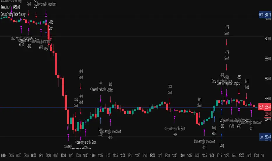
ICT Master Suite [Trading IQ]Hello Traders!
We’re excited to introduce the ICT Master Suite by TradingIQ, a new tool designed to bring together several ICT concepts and strategies in one place.
The Purpose Behind the ICT Master Suite
There are a few challenges traders often face when using ICT-related indicators:
Many available indicators focus on one or two ICT methods, which can limit traders who apply a broader range of ICT related techniques on their charts.
There aren't many indicators for ICT strategy models, and we couldn't find ICT indicators that allow for testing the strategy models and setting alerts.
Many ICT related concepts exist in the public domain as indicators, not strategies! This makes it difficult to verify that the ICT concept has some utility in the market you're trading and if it's worth trading - it's difficult to know if it's working!
Some users might not have enough chart space to apply numerous ICT related indicators, which can be restrictive for those wanting to use multiple ICT techniques simultaneously.
The ICT Master Suite is designed to offer a comprehensive option for traders who want to apply a variety of ICT methods. By combining several ICT techniques and strategy models into one indicator, it helps users maximize their chart space while accessing multiple tools in a single slot.
Additionally, the ICT Master Suite was developed as a strategy . This means users can backtest various ICT strategy models - including deep backtesting. A primary goal of this indicator is to let traders decide for themselves what markets to trade ICT concepts in and give them the capability to figure out if the strategy models are worth trading!
What Makes the ICT Master Suite Different
There are many ICT-related indicators available on TradingView, each offering valuable insights. What the ICT Master Suite aims to do is bring together a wider selection of these techniques into one tool. This includes both key ICT methods and strategy models, allowing traders to test and activate strategies all within one indicator.
Features
The ICT Master Suite offers:
Multiple ICT strategy models, including the 2022 Strategy Model and Unicorn Model, which can be built, tested, and used for live trading.
Calculation and display of key price areas like Breaker Blocks, Rejection Blocks, Order Blocks, Fair Value Gaps, Equal Levels, and more.
The ability to set alerts based on these ICT strategies and key price areas.
A comprehensive, yet practical, all-inclusive ICT indicator for traders.
Customizable Timeframe - Calculate ICT concepts on off-chart timeframes
Unicorn Strategy Model
2022 Strategy Model
Liquidity Raid Strategy Model
OTE (Optimal Trade Entry) Strategy Model
Silver Bullet Strategy Model
Order blocks
Breaker blocks
Rejection blocks
FVG
Strong highs and lows
Displacements
Liquidity sweeps
Power of 3
ICT Macros
HTF previous bar high and low
Break of Structure indications
Market Structure Shift indications
Equal highs and lows
Swings highs and swing lows
Fibonacci TPs and SLs
Swing level TPs and SLs
Previous day high and low TPs and SLs
And much more! An ongoing project!
How To Use
Many traders will already be familiar with the ICT related concepts listed above, and will find using the ICT Master Suite quite intuitive!
Despite this, let's go over the features of the tool in-depth and how to use the tool!
The image above shows the ICT Master Suite with almost all techniques activated.
ICT 2022 Strategy Model
The ICT Master suite provides the ability to test, set alerts for, and live trade the ICT 2022 Strategy Model.
The image above shows an example of a long position being entered following a complete setup for the 2022 ICT model.
A liquidity sweep occurs prior to an upside breakout. During the upside breakout the model looks for the FVG that is nearest 50% of the setup range. A limit order is placed at this FVG for entry.
The target entry percentage for the range is customizable in the settings. For instance, you can select to enter at an FVG nearest 33% of the range, 20%, 66%, etc.
The profit target for the model generally uses the highest high of the range (100%) for longs and the lowest low of the range (100%) for shorts. Stop losses are generally set at 0% of the range.
The image above shows the short model in action!
Whether you decide to follow the 2022 model diligently or not, you can still set alerts when the entry condition is met.
ICT Unicorn Model
The image above shows an example of a long position being entered following a complete setup for the ICT Unicorn model.
A lower swing low followed by a higher swing high precedes the overlap of an FVG and breaker block formed during the sequence.
During the upside breakout the model looks for an FVG and breaker block that formed during the sequence and overlap each other. A limit order is placed at the nearest overlap point to current price.
The profit target for this example trade is set at the swing high and the stop loss at the swing low. However, both the profit target and stop loss for this model are configurable in the settings.
For Longs, the selectable profit targets are:
Swing High
Fib -0.5
Fib -1
Fib -2
For Longs, the selectable stop losses are:
Swing Low
Bottom of FVG or breaker block
The image above shows the short version of the Unicorn Model in action!
For Shorts, the selectable profit targets are:
Swing Low
Fib -0.5
Fib -1
Fib -2
For Shorts, the selectable stop losses are:
Swing High
Top of FVG or breaker block
The image above shows the profit target and stop loss options in the settings for the Unicorn Model.
Optimal Trade Entry (OTE) Model
The image above shows an example of a long position being entered following a complete setup for the OTE model.
Price retraces either 0.62, 0.705, or 0.79 of an upside move and a trade is entered.
The profit target for this example trade is set at the -0.5 fib level. This is also adjustable in the settings.
For Longs, the selectable profit targets are:
Swing High
Fib -0.5
Fib -1
Fib -2
The image above shows the short version of the OTE Model in action!
For Shorts, the selectable profit targets are:
Swing Low
Fib -0.5
Fib -1
Fib -2
Liquidity Raid Model
The image above shows an example of a long position being entered following a complete setup for the Liquidity Raid Modell.
The user must define the session in the settings (for this example it is 13:30-16:00 NY time).
During the session, the indicator will calculate the session high and session low. Following a “raid” of either the session high or session low (after the session has completed) the script will look for an entry at a recently formed breaker block.
If the session high is raided the script will look for short entries at a bearish breaker block. If the session low is raided the script will look for long entries at a bullish breaker block.
For Longs, the profit target options are:
Swing high
User inputted Lib level
For Longs, the stop loss options are:
Swing low
User inputted Lib level
Breaker block bottom
The image above shows the short version of the Liquidity Raid Model in action!
For Shorts, the profit target options are:
Swing Low
User inputted Lib level
For Shorts, the stop loss options are:
Swing High
User inputted Lib level
Breaker block top
Silver Bullet Model
The image above shows an example of a long position being entered following a complete setup for the Silver Bullet Modell.
During the session, the indicator will determine the higher timeframe bias. If the higher timeframe bias is bullish the strategy will look to enter long at an FVG that forms during the session. If the higher timeframe bias is bearish the indicator will look to enter short at an FVG that forms during the session.
For Longs, the profit target options are:
Nearest Swing High Above Entry
Previous Day High
For Longs, the stop loss options are:
Nearest Swing Low
Previous Day Low
The image above shows the short version of the Silver Bullet Model in action!
For Shorts, the profit target options are:
Nearest Swing Low Below Entry
Previous Day Low
For Shorts, the stop loss options are:
Nearest Swing High
Previous Day High
Order blocks
The image above shows indicator identifying and labeling order blocks.
The color of the order blocks, and how many should be shown, are configurable in the settings!
Breaker Blocks
The image above shows indicator identifying and labeling order blocks.
The color of the breaker blocks, and how many should be shown, are configurable in the settings!
Rejection Blocks
The image above shows indicator identifying and labeling rejection blocks.
The color of the rejection blocks, and how many should be shown, are configurable in the settings!
Fair Value Gaps
The image above shows indicator identifying and labeling fair value gaps.
The color of the fair value gaps, and how many should be shown, are configurable in the settings!
Additionally, you can select to only show fair values gaps that form after a liquidity sweep. Doing so reduces "noisy" FVGs and focuses on identifying FVGs that form after a significant trading event.
The image above shows the feature enabled. A fair value gap that occurred after a liquidity sweep is shown.
Market Structure
The image above shows the ICT Master Suite calculating market structure shots and break of structures!
The color of MSS and BoS, and whether they should be displayed, are configurable in the settings.
Displacements
The images above show indicator identifying and labeling displacements.
The color of the displacements, and how many should be shown, are configurable in the settings!
Equal Price Points
The image above shows the indicator identifying and labeling equal highs and equal lows.
The color of the equal levels, and how many should be shown, are configurable in the settings!
Previous Custom TF High/Low
The image above shows the ICT Master Suite calculating the high and low price for a user-defined timeframe. In this case the previous day’s high and low are calculated.
To illustrate the customizable timeframe function, the image above shows the indicator calculating the previous 4 hour high and low.
Liquidity Sweeps
The image above shows the indicator identifying a liquidity sweep prior to an upside breakout.
The image above shows the indicator identifying a liquidity sweep prior to a downside breakout.
The color and aggressiveness of liquidity sweep identification are adjustable in the settings!
Power Of Three
The image above shows the indicator calculating Po3 for two user-defined higher timeframes!
Macros
The image above shows the ICT Master Suite identifying the ICT macros!
ICT Macros are only displayable on the 5 minute timeframe or less.
Strategy Performance Table
In addition to a full-fledged TradingView backtest for any of the ICT strategy models the indicator offers, a quick-and-easy strategy table exists for the indicator!
The image above shows the strategy performance table in action.
Keep in mind that, because the ICT Master Suite is a strategy script, you can perform fully automatic backtests, deep backtests, easily add commission and portfolio balance and look at pertinent metrics for the ICT strategies you are testing!
Lite Mode
Traders who want the cleanest chart possible can toggle on “Lite Mode”!
In Lite Mode, any neon or “glow” like effects are removed and key levels are marked as strict border boxes. You can also select to remove box borders if that’s what you prefer!
Settings Used For Backtest
For the displayed backtest, a starting balance of $1000 USD was used. A commission of 0.02%, slippage of 2 ticks, a verify price for limit orders of 2 ticks, and 5% of capital investment per order.
A commission of 0.02% was used due to the backtested asset being a perpetual future contract for a crypto currency. The highest commission (lowest-tier VIP) for maker orders on many exchanges is 0.02%. All entered positions take place as maker orders and so do profit target exits. Stop orders exist as stop-market orders.
A slippage of 2 ticks was used to simulate more realistic stop-market orders. A verify limit order settings of 2 ticks was also used. Even though BTCUSDT.P on Binance is liquid, we just want the backtest to be on the safe side. Additionally, the backtest traded 100+ trades over the period. The higher the sample size the better; however, this example test can serve as a starting point for traders interested in ICT concepts.
Community Assistance And Feedback
Given the complexity and idiosyncratic applications of ICT concepts amongst its proponents, the ICT Master Suite’s built-in strategies and level identification methods might not align with everyone's interpretation.
That said, the best we can do is precisely define ICT strategy rules and concepts to a repeatable process, test, and apply them! Whether or not an ICT strategy is trading precisely how you would trade it, seeing the model in action, taking trades, and with performance statistics is immensely helpful in assessing predictive utility.
If you think we missed something, you notice a bug, have an idea for strategy model improvement, please let us know! The ICT Master Suite is an ongoing project that will, ideally, be shaped by the community.
A big thank you to the @PineCoders for their Time Library!
Thank you!
Trailing Take Profit - Close Based📝 Description
This script demonstrates a new approach to the trailing take profit.
Trailing Take Profit is a price-following technique. When used, instead of setting a limit order for the take profit target exiting from your position at the specified price, a stop order is conditionally set when the take profit target is reached. Then, the stop price (a.k.a trailing price), is placed below the take profit target at a distance defined by the user percentagewise. On regular time intervals, the stop price gets updated by following the "Trail Barrier" price (high by default) upwards. When the current price hits the stop price you exit the trade. Check the chart for more details.
This script demonstrates how to implement the close-based Trailing Take Profit logic for long positions, but it can also be applied for short positions if the logic is "reversed".
📢 NOTE
To generate some entries and showcase the "Trailing Take Profit" technique, this script uses the crossing of two moving averages. Please keep in mind that you should not relate the Backtesting results you see in the "Strategy Tester" tab with the success of the technique itself.
This is not a complete strategy per se, and the backtest results are affected by many parameters that are outside of the scope of this publication. If you choose to use this new approach of the "Trailing Take Profit" in your logic you have to make sure that you are backtesting the whole strategy.
⚔️ Comparison
In contrast to my older "Trailing Take Profit" publication where the trailing take profit implementation was tick-based, this new approach is close-based, meaning that the update of the stop price occurs at the bar close instead of every tick.
While comparing the real-time results of the two implementations is like comparing apples to oranges, because they have different dynamic behavior, the new approach offers better consistency between the backtesting results and the real-time results.
By updating the stop price on every bar close, you do not rely on the backtester assumptions anymore (check the Reasoning section below for more info).
The new approach resembles the conditional "Trailing Exit" technique, where the condition is true when the current price crosses over the take profit target. Then, the stop order is placed at the trailing price and it gets updated on every bar close to "follow" the barrier price (high). On the other hand, the older tick-based approach had more "tight" dynamics since the trailing price gets updated on every tick leaving less room for price fluctuations by making it more probable to reach the trailing price.
🤔 Reasoning
This new close-based approach addresses several practical issues the older tick-based approach had. Those issues arise mainly from the technicalities of the TV Backtester. More specifically, due to the assumptions the Broker Emulator makes for the price action of the history bars, the backtesting results in the TV Backtester are exaggerated, and depending on the timeframe, the backtesting results look way better than they are in reality.
The effect above, and the inability to reason about the performance of a strategy separated people into two groups. Those who never use this feature, because they couldn't know for sure the actual effect it might have in their strategy, (even if it turned out to be more profitable) and those who abused this type of "repainting" behavior to show off, and hijack some boosts from the community by boasting about the "fake" results of their strategies.
Even if there are ways to evaluate the effectiveness of the tick-based approach that is applied in an existing strategy (this is out of the topic of this publication), it requires extra effort to do the analysis. Using this closed-based approach we can have more predictable results, without surprises.
⚠️ Caveats
Since this approach updates the trailing price on bar close, you must wait for at least one bar to close after the price crosses over the take profit target.
Alert(), alertcondition() or strategy alerts?Variety of possibilities offered by PineScript, especially thanks to recent additions, created some confusion. Especially one question repeats quite often - which method to use to trigger alerts?
I'm posting this to clarify and give some syntax examples. I'll discuss these 3 methods in chronological order, meaning - in the order they were introduced to PineScript.
ALERTCONDITION() - it is a function call, which can be used only in study-type script. Since years ago, you could create 2 types of a script: strategy and study. First one enables creating a backtest of a strategy. Second was to develop scripts which didn't require backtesting and could trigger alerts. alertcondition() calls in strategy-type scripts were rejected by Pine compiler. On the other hand compiling study-type scripts rejected all strategy...() calls. That created difficulties, because once you had a nice and backtested strategy, you had to rip it off from all strategy...() function calls to convert your script to study-type so you could produce alerts. Maintenance of two versions of each script was necessary and it was painful.
"STRATEGY ALERTS" were introduced because of alertcondition() pains. To create strategy alert, you need to click "Add alert" button inside Strategy Tester (backtester) and only there. Alerts set-up this way are bound with the backtester - whenever backtester triggers an order, which is visible on the chart, alert is also fired. And you can customize alert message using some placeholders like {{strategy.order.contracts}} or {{ticker}}.
ALERT() was added last. This is an alerts-triggering function call, which can be run from strategy-type script. Finally it is doable! You can connect it to any event coded in PineScript and generate any alert message you want, thanks to concatenation of strings and wrapping variables into tostring() function.
Out of these three alertcondition() is obviously archaic and probably will be discontinued. There is a chance this makes strategy/study distinction not making sense anymore, so I wouldn't be surprised if "studies" are deprecated at some point.
But what are the differences between "Strategy alerts" and alert()? "Strategy alerts" seem easier to set-up with just a few clicks and probably easier to understand and verify, because they go in sync with the backtester and on-chart trade markers. It is especially important to understand how they work if you're building strategy based on pending orders (stop and limit) - events in your code might trigger placing pending order, but alert will be triggered only (and when) such order is executed.
But "Strategy Alerts" have some limitations - not every variable you'd like to include in alert message is available from PineScript. And maybe you don't need the alert fired when the trade hit a stop-loss or take-profit, because you have already forwarded info about closing conditions in entry alert to your broker/exchange.
Alert() was added to PineScript to fill all these gaps. Is allows concatenating any alert message you want, with any variable you want inside it and you can attach alert() function at any event in your PineScript code. For example - when placing orders, crossing variables, exiting trades, but not explicitly at pending orders execution.
The Verdict
"Strategy Alerts" might seem a better fit - easier to set-up and verify, flexible and they fire only when a trade really happens, not producing unnecessary mess when each pending order is placed. But these advantages are illusionary, because they don't give you the full-control which is needed when trading with real money. Especially when using pending orders. If an alert is fired when price actually hit a stop-order or limit-order level, and even if you are executing such alert within 1 second thanks to a tool like TradingConnector, you might already be late and you are making entry at a market price. Slippage will play a great role here. You need to send ordering alert when logical conditions are met - then it will be executed at the price you want. Even if you need to cancel all the pending orders which were not executed. Because of that I strongly recommend sticking to ALERT() when building your alerts system.
Below is an example strategy, showing syntax to manage placing the orders and cancelling them. Yes, this is another spin-off from my TradingView Alerts to MT4 MT5 . As usual, please don't pay attention to backtest results, as this is educational script only.
P.S. For the last time - farewell alertcondition(). You served us well.
Zero Lag Trend Signals (MTF) [Quant Trading] V7Overview
The Zero Lag Trend Signals (MTF) V7 is a comprehensive trend-following strategy that combines Zero Lag Exponential Moving Average (ZLEMA) with volatility-based bands to identify high-probability trade entries and exits. This strategy is designed to reduce lag inherent in traditional moving averages while incorporating dynamic risk management through ATR-based stops and multiple exit mechanisms.
This is a longer term horizon strategy that takes limited trades. It is not a high frequency trading and therefore will also have limited data and not > 100 trades.
How It Works
Core Signal Generation:
The strategy uses a Zero Lag EMA (ZLEMA) calculated by applying an EMA to price data that has been adjusted for lag:
Calculate lag period: floor((length - 1) / 2)
Apply lag correction: src + (src - src )
Calculate ZLEMA: EMA of lag-corrected price
Volatility bands are created using the highest ATR over a lookback period multiplied by a band multiplier. These bands are added to and subtracted from the ZLEMA line to create upper and lower boundaries.
Trend Detection:
The strategy maintains a trend variable that switches between bullish (1) and bearish (-1):
Long Signal: Triggers when price crosses above ZLEMA + volatility band
Short Signal: Triggers when price crosses below ZLEMA - volatility band
Optional ZLEMA Trend Confirmation:
When enabled, this filter requires ZLEMA to show directional momentum before entry:
Bullish Confirmation: ZLEMA must increase for 4 consecutive bars
Bearish Confirmation: ZLEMA must decrease for 4 consecutive bars
This additional filter helps avoid false signals in choppy or ranging markets.
Risk Management Features:
The strategy includes multiple stop-loss and take-profit mechanisms:
Volatility-Based Stops: Default stop-loss is placed at ZLEMA ± volatility band
ATR-Based Stops: Dynamic stop-loss calculated as entry price ± (ATR × multiplier)
ATR Trailing Stop: Ratcheting stop-loss that follows price but never moves against position
Risk-Reward Profit Target: Take-profit level set as a multiple of stop distance
Break-Even Stop: Moves stop to entry price after reaching specified R:R ratio
Trend-Based Exit: Closes position when price crosses EMA in opposite direction
Performance Tracking:
The strategy includes optional features for monitoring and analyzing trades:
Floating Statistics Table: Displays key metrics including win rate, GOA (Gain on Account), net P&L, and max drawdown
Trade Log Labels: Shows entry/exit prices, P&L, bars held, and exit reason for each closed trade
CSV Export Fields: Outputs trade data for external analysis
Default Strategy Settings
Commission & Slippage:
Commission: 0.1% per trade
Slippage: 3 ticks
Initial Capital: $1,000
Position Size: 100% of equity per trade
Main Calculation Parameters:
Length: 70 (range: 70-7000) - Controls ZLEMA calculation period
Band Multiplier: 1.2 - Adjusts width of volatility bands
Entry Conditions (All Disabled by Default):
Use ZLEMA Trend Confirmation: OFF - Requires ZLEMA directional momentum
Re-Enter on Long Trend: OFF - Allows multiple entries during sustained trends
Short Trades:
Allow Short Trades: OFF - Strategy is long-only by default
Performance Settings (All Disabled by Default):
Use Profit Target: OFF
Profit Target Risk-Reward Ratio: 2.0 (when enabled)
Dynamic TP/SL (All Disabled by Default):
Use ATR-Based Stop-Loss & Take-Profit: OFF
ATR Length: 14
Stop-Loss ATR Multiplier: 1.5
Profit Target ATR Multiplier: 2.5
Use ATR Trailing Stop: OFF
Trailing Stop ATR Multiplier: 1.5
Use Break-Even Stop-Loss: OFF
Move SL to Break-Even After RR: 1.5
Use Trend-Based Take Profit: OFF
EMA Exit Length: 9
Trade Data Display (All Disabled by Default):
Show Floating Stats Table: OFF
Show Trade Log Labels: OFF
Enable CSV Export: OFF
Trade Label Vertical Offset: 0.5
Backtesting Date Range:
Start Date: January 1, 2018
End Date: December 31, 2069
Important Usage Notes
Default Configuration: The strategy operates in its most basic form with default settings - using only ZLEMA crossovers with volatility bands and volatility-based stop-losses. All advanced features must be manually enabled.
Stop-Loss Priority: If multiple stop-loss methods are enabled simultaneously, the strategy will use whichever condition is hit first. ATR-based stops override volatility-based stops when enabled.
Long-Only by Default: Short trading is disabled by default. Enable "Allow Short Trades" to trade both directions.
Performance Monitoring: Enable the floating stats table and trade log labels to visualize strategy performance during backtesting.
Exit Mechanisms: The strategy can exit trades through multiple methods: stop-loss hit, take-profit reached, trend reversal, or trailing stop activation. The trade log identifies which exit method was used.
Re-Entry Logic: When "Re-Enter on Long Trend" is enabled with ZLEMA trend confirmation, the strategy can take multiple long positions during extended uptrends as long as all entry conditions remain valid.
Capital Efficiency: Default setting uses 100% of equity per trade. Adjust "default_qty_value" to manage position sizing based on risk tolerance.
Realistic Backtesting: Strategy includes commission (0.1%) and slippage (3 ticks) to provide realistic performance expectations. These values should be adjusted based on your broker and market conditions.
Recommended Use Cases
Trending Markets: Best suited for markets with clear directional moves where trend-following strategies excel
Medium to Long-Term Trading: The default length of 70 makes this strategy more appropriate for swing trading rather than scalping
Risk-Conscious Traders: Multiple stop-loss options allow traders to customize risk management to their comfort level
Backtesting & Optimization: Comprehensive performance tracking features make this strategy ideal for testing different parameter combinations
Limitations & Considerations
Like all trend-following strategies, performance may suffer in choppy or ranging markets
Default 100% position sizing means full capital exposure per trade - consider reducing for conservative risk management
Higher length values (70+) reduce signal frequency but may improve signal quality
Multiple simultaneous risk management features may create conflicting exit signals
Past performance shown in backtests does not guarantee future results
Customization Tips
For more aggressive trading:
Reduce length parameter (minimum 70)
Decrease band multiplier for tighter bands
Enable short trades
Use lower profit target R:R ratios
For more conservative trading:
Increase length parameter
Enable ZLEMA trend confirmation
Use wider ATR stop-loss multipliers
Enable break-even stop-loss
Reduce position size from 100% default
For optimal choppy market performance:
Enable ZLEMA trend confirmation
Increase band multiplier
Use tighter profit targets
Avoid re-entry on trend continuation
Visual Elements
The strategy plots several elements on the chart:
ZLEMA line (color-coded by trend direction)
Upper and lower volatility bands
Long entry markers (green triangles)
Short entry markers (red triangles, when enabled)
Stop-loss levels (when positions are open)
Take-profit levels (when enabled and positions are open)
Trailing stop lines (when enabled and positions are open)
Optional ZLEMA trend markers (triangles at highs/lows)
Optional trade log labels showing complete trade information
Exit Reason Codes (for CSV Export)
When CSV export is enabled, exit reasons are coded as:
0 = Manual/Other
1 = Trailing Stop-Loss
2 = Profit Target
3 = ATR Stop-Loss
4 = Trend Change
Conclusion
Zero Lag Trend Signals V7 provides a robust framework for trend-following with extensive customization options. The strategy balances simplicity in its core logic with sophisticated risk management features, making it suitable for both beginner and advanced traders. By reducing moving average lag while incorporating volatility-based signals, it aims to capture trends earlier while managing risk through multiple configurable exit mechanisms.
The modular design allows traders to start with basic trend-following and progressively add complexity through ZLEMA confirmation, multiple stop-loss methods, and advanced exit strategies. Comprehensive performance tracking and export capabilities make this strategy an excellent tool for systematic testing and optimization.
Note: This strategy is provided for educational and backtesting purposes. All trading involves risk. Past performance does not guarantee future results. Always test thoroughly with paper trading before risking real capital, and adjust position sizing and risk parameters according to your risk tolerance and account size.
================================================================================
TAGS:
================================================================================
trend following, ZLEMA, zero lag, volatility bands, ATR stops, risk management, swing trading, momentum, trend confirmation, backtesting
================================================================================
CATEGORY:
================================================================================
Strategies
================================================================================
CHART SETUP RECOMMENDATIONS:
================================================================================
For optimal visualization when publishing:
Use a clean chart with no other indicators overlaid
Select a timeframe that shows multiple trade signals (4H or Daily recommended)
Choose a trending asset (crypto, forex major pairs, or trending stocks work well)
Show at least 6-12 months of data to demonstrate strategy across different market conditions
Enable the floating stats table to display key performance metrics
Ensure all indicator lines (ZLEMA, bands, stops) are clearly visible
Use the default chart type (candlesticks) - avoid Heikin Ashi, Renko, etc.
Make sure symbol information and timeframe are clearly visible
================================================================================
COMPLIANCE NOTES:
================================================================================
✅ Open-source publication with complete code visibility
✅ English-only title and description
✅ Detailed explanation of methodology and calculations
✅ Realistic commission (0.1%) and slippage (3 ticks) included
✅ All default parameters clearly documented
✅ Performance limitations and risks disclosed
✅ No unrealistic claims about performance
✅ No guaranteed results promised
✅ Appropriate for public library (original trend-following implementation with ZLEMA)
✅ Educational disclaimers included
✅ All features explained in detail
================================================================================
Markov Chain [3D] | FractalystWhat exactly is a Markov Chain?
This indicator uses a Markov Chain model to analyze, quantify, and visualize the transitions between market regimes (Bull, Bear, Neutral) on your chart. It dynamically detects these regimes in real-time, calculates transition probabilities, and displays them as animated 3D spheres and arrows, giving traders intuitive insight into current and future market conditions.
How does a Markov Chain work, and how should I read this spheres-and-arrows diagram?
Think of three weather modes: Sunny, Rainy, Cloudy.
Each sphere is one mode. The loop on a sphere means “stay the same next step” (e.g., Sunny again tomorrow).
The arrows leaving a sphere show where things usually go next if they change (e.g., Sunny moving to Cloudy).
Some paths matter more than others. A more prominent loop means the current mode tends to persist. A more prominent outgoing arrow means a change to that destination is the usual next step.
Direction isn’t symmetric: moving Sunny→Cloudy can behave differently than Cloudy→Sunny.
Now relabel the spheres to markets: Bull, Bear, Neutral.
Spheres: market regimes (uptrend, downtrend, range).
Self‑loop: tendency for the current regime to continue on the next bar.
Arrows: the most common next regime if a switch happens.
How to read: Start at the sphere that matches current bar state. If the loop stands out, expect continuation. If one outgoing path stands out, that switch is the typical next step. Opposite directions can differ (Bear→Neutral doesn’t have to match Neutral→Bear).
What states and transitions are shown?
The three market states visualized are:
Bullish (Bull): Upward or strong-market regime.
Bearish (Bear): Downward or weak-market regime.
Neutral: Sideways or range-bound regime.
Bidirectional animated arrows and probability labels show how likely the market is to move from one regime to another (e.g., Bull → Bear or Neutral → Bull).
How does the regime detection system work?
You can use either built-in price returns (based on adaptive Z-score normalization) or supply three custom indicators (such as volume, oscillators, etc.).
Values are statistically normalized (Z-scored) over a configurable lookback period.
The normalized outputs are classified into Bull, Bear, or Neutral zones.
If using three indicators, their regime signals are averaged and smoothed for robustness.
How are transition probabilities calculated?
On every confirmed bar, the algorithm tracks the sequence of detected market states, then builds a rolling window of transitions.
The code maintains a transition count matrix for all regime pairs (e.g., Bull → Bear).
Transition probabilities are extracted for each possible state change using Laplace smoothing for numerical stability, and frequently updated in real-time.
What is unique about the visualization?
3D animated spheres represent each regime and change visually when active.
Animated, bidirectional arrows reveal transition probabilities and allow you to see both dominant and less likely regime flows.
Particles (moving dots) animate along the arrows, enhancing the perception of regime flow direction and speed.
All elements dynamically update with each new price bar, providing a live market map in an intuitive, engaging format.
Can I use custom indicators for regime classification?
Yes! Enable the "Custom Indicators" switch and select any three chart series as inputs. These will be normalized and combined (each with equal weight), broadening the regime classification beyond just price-based movement.
What does the “Lookback Period” control?
Lookback Period (default: 100) sets how much historical data builds the probability matrix. Shorter periods adapt faster to regime changes but may be noisier. Longer periods are more stable but slower to adapt.
How is this different from a Hidden Markov Model (HMM)?
It sets the window for both regime detection and probability calculations. Lower values make the system more reactive, but potentially noisier. Higher values smooth estimates and make the system more robust.
How is this Markov Chain different from a Hidden Markov Model (HMM)?
Markov Chain (as here): All market regimes (Bull, Bear, Neutral) are directly observable on the chart. The transition matrix is built from actual detected regimes, keeping the model simple and interpretable.
Hidden Markov Model: The actual regimes are unobservable ("hidden") and must be inferred from market output or indicator "emissions" using statistical learning algorithms. HMMs are more complex, can capture more subtle structure, but are harder to visualize and require additional machine learning steps for training.
A standard Markov Chain models transitions between observable states using a simple transition matrix, while a Hidden Markov Model assumes the true states are hidden (latent) and must be inferred from observable “emissions” like price or volume data. In practical terms, a Markov Chain is transparent and easier to implement and interpret; an HMM is more expressive but requires statistical inference to estimate hidden states from data.
Markov Chain: states are observable; you directly count or estimate transition probabilities between visible states. This makes it simpler, faster, and easier to validate and tune.
HMM: states are hidden; you only observe emissions generated by those latent states. Learning involves machine learning/statistical algorithms (commonly Baum–Welch/EM for training and Viterbi for decoding) to infer both the transition dynamics and the most likely hidden state sequence from data.
How does the indicator avoid “repainting” or look-ahead bias?
All regime changes and matrix updates happen only on confirmed (closed) bars, so no future data is leaked, ensuring reliable real-time operation.
Are there practical tuning tips?
Tune the Lookback Period for your asset/timeframe: shorter for fast markets, longer for stability.
Use custom indicators if your asset has unique regime drivers.
Watch for rapid changes in transition probabilities as early warning of a possible regime shift.
Who is this indicator for?
Quants and quantitative researchers exploring probabilistic market modeling, especially those interested in regime-switching dynamics and Markov models.
Programmers and system developers who need a probabilistic regime filter for systematic and algorithmic backtesting:
The Markov Chain indicator is ideally suited for programmatic integration via its bias output (1 = Bull, 0 = Neutral, -1 = Bear).
Although the visualization is engaging, the core output is designed for automated, rules-based workflows—not for discretionary/manual trading decisions.
Developers can connect the indicator’s output directly to their Pine Script logic (using input.source()), allowing rapid and robust backtesting of regime-based strategies.
It acts as a plug-and-play regime filter: simply plug the bias output into your entry/exit logic, and you have a scientifically robust, probabilistically-derived signal for filtering, timing, position sizing, or risk regimes.
The MC's output is intentionally "trinary" (1/0/-1), focusing on clear regime states for unambiguous decision-making in code. If you require nuanced, multi-probability or soft-label state vectors, consider expanding the indicator or stacking it with a probability-weighted logic layer in your scripting.
Because it avoids subjectivity, this approach is optimal for systematic quants, algo developers building backtested, repeatable strategies based on probabilistic regime analysis.
What's the mathematical foundation behind this?
The mathematical foundation behind this Markov Chain indicator—and probabilistic regime detection in finance—draws from two principal models: the (standard) Markov Chain and the Hidden Markov Model (HMM).
How to use this indicator programmatically?
The Markov Chain indicator automatically exports a bias value (+1 for Bullish, -1 for Bearish, 0 for Neutral) as a plot visible in the Data Window. This allows you to integrate its regime signal into your own scripts and strategies for backtesting, automation, or live trading.
Step-by-Step Integration with Pine Script (input.source)
Add the Markov Chain indicator to your chart.
This must be done first, since your custom script will "pull" the bias signal from the indicator's plot.
In your strategy, create an input using input.source()
Example:
//@version=5
strategy("MC Bias Strategy Example")
mcBias = input.source(close, "MC Bias Source")
After saving, go to your script’s settings. For the “MC Bias Source” input, select the plot/output of the Markov Chain indicator (typically its bias plot).
Use the bias in your trading logic
Example (long only on Bull, flat otherwise):
if mcBias == 1
strategy.entry("Long", strategy.long)
else
strategy.close("Long")
For more advanced workflows, combine mcBias with additional filters or trailing stops.
How does this work behind-the-scenes?
TradingView’s input.source() lets you use any plot from another indicator as a real-time, “live” data feed in your own script (source).
The selected bias signal is available to your Pine code as a variable, enabling logical decisions based on regime (trend-following, mean-reversion, etc.).
This enables powerful strategy modularity : decouple regime detection from entry/exit logic, allowing fast experimentation without rewriting core signal code.
Integrating 45+ Indicators with Your Markov Chain — How & Why
The Enhanced Custom Indicators Export script exports a massive suite of over 45 technical indicators—ranging from classic momentum (RSI, MACD, Stochastic, etc.) to trend, volume, volatility, and oscillator tools—all pre-calculated, centered/scaled, and available as plots.
// Enhanced Custom Indicators Export - 45 Technical Indicators
// Comprehensive technical analysis suite for advanced market regime detection
//@version=6
indicator('Enhanced Custom Indicators Export | Fractalyst', shorttitle='Enhanced CI Export', overlay=false, scale=scale.right, max_labels_count=500, max_lines_count=500)
// |----- Input Parameters -----| //
momentum_group = "Momentum Indicators"
trend_group = "Trend Indicators"
volume_group = "Volume Indicators"
volatility_group = "Volatility Indicators"
oscillator_group = "Oscillator Indicators"
display_group = "Display Settings"
// Common lengths
length_14 = input.int(14, "Standard Length (14)", minval=1, maxval=100, group=momentum_group)
length_20 = input.int(20, "Medium Length (20)", minval=1, maxval=200, group=trend_group)
length_50 = input.int(50, "Long Length (50)", minval=1, maxval=200, group=trend_group)
// Display options
show_table = input.bool(true, "Show Values Table", group=display_group)
table_size = input.string("Small", "Table Size", options= , group=display_group)
// |----- MOMENTUM INDICATORS (15 indicators) -----| //
// 1. RSI (Relative Strength Index)
rsi_14 = ta.rsi(close, length_14)
rsi_centered = rsi_14 - 50
// 2. Stochastic Oscillator
stoch_k = ta.stoch(close, high, low, length_14)
stoch_d = ta.sma(stoch_k, 3)
stoch_centered = stoch_k - 50
// 3. Williams %R
williams_r = ta.stoch(close, high, low, length_14) - 100
// 4. MACD (Moving Average Convergence Divergence)
= ta.macd(close, 12, 26, 9)
// 5. Momentum (Rate of Change)
momentum = ta.mom(close, length_14)
momentum_pct = (momentum / close ) * 100
// 6. Rate of Change (ROC)
roc = ta.roc(close, length_14)
// 7. Commodity Channel Index (CCI)
cci = ta.cci(close, length_20)
// 8. Money Flow Index (MFI)
mfi = ta.mfi(close, length_14)
mfi_centered = mfi - 50
// 9. Awesome Oscillator (AO)
ao = ta.sma(hl2, 5) - ta.sma(hl2, 34)
// 10. Accelerator Oscillator (AC)
ac = ao - ta.sma(ao, 5)
// 11. Chande Momentum Oscillator (CMO)
cmo = ta.cmo(close, length_14)
// 12. Detrended Price Oscillator (DPO)
dpo = close - ta.sma(close, length_20)
// 13. Price Oscillator (PPO)
ppo = ta.sma(close, 12) - ta.sma(close, 26)
ppo_pct = (ppo / ta.sma(close, 26)) * 100
// 14. TRIX
trix_ema1 = ta.ema(close, length_14)
trix_ema2 = ta.ema(trix_ema1, length_14)
trix_ema3 = ta.ema(trix_ema2, length_14)
trix = ta.roc(trix_ema3, 1) * 10000
// 15. Klinger Oscillator
klinger = ta.ema(volume * (high + low + close) / 3, 34) - ta.ema(volume * (high + low + close) / 3, 55)
// 16. Fisher Transform
fisher_hl2 = 0.5 * (hl2 - ta.lowest(hl2, 10)) / (ta.highest(hl2, 10) - ta.lowest(hl2, 10)) - 0.25
fisher = 0.5 * math.log((1 + fisher_hl2) / (1 - fisher_hl2))
// 17. Stochastic RSI
stoch_rsi = ta.stoch(rsi_14, rsi_14, rsi_14, length_14)
stoch_rsi_centered = stoch_rsi - 50
// 18. Relative Vigor Index (RVI)
rvi_num = ta.swma(close - open)
rvi_den = ta.swma(high - low)
rvi = rvi_den != 0 ? rvi_num / rvi_den : 0
// 19. Balance of Power (BOP)
bop = (close - open) / (high - low)
// |----- TREND INDICATORS (10 indicators) -----| //
// 20. Simple Moving Average Momentum
sma_20 = ta.sma(close, length_20)
sma_momentum = ((close - sma_20) / sma_20) * 100
// 21. Exponential Moving Average Momentum
ema_20 = ta.ema(close, length_20)
ema_momentum = ((close - ema_20) / ema_20) * 100
// 22. Parabolic SAR
sar = ta.sar(0.02, 0.02, 0.2)
sar_trend = close > sar ? 1 : -1
// 23. Linear Regression Slope
lr_slope = ta.linreg(close, length_20, 0) - ta.linreg(close, length_20, 1)
// 24. Moving Average Convergence (MAC)
mac = ta.sma(close, 10) - ta.sma(close, 30)
// 25. Trend Intensity Index (TII)
tii_sum = 0.0
for i = 1 to length_20
tii_sum += close > close ? 1 : 0
tii = (tii_sum / length_20) * 100
// 26. Ichimoku Cloud Components
ichimoku_tenkan = (ta.highest(high, 9) + ta.lowest(low, 9)) / 2
ichimoku_kijun = (ta.highest(high, 26) + ta.lowest(low, 26)) / 2
ichimoku_signal = ichimoku_tenkan > ichimoku_kijun ? 1 : -1
// 27. MESA Adaptive Moving Average (MAMA)
mama_alpha = 2.0 / (length_20 + 1)
mama = ta.ema(close, length_20)
mama_momentum = ((close - mama) / mama) * 100
// 28. Zero Lag Exponential Moving Average (ZLEMA)
zlema_lag = math.round((length_20 - 1) / 2)
zlema_data = close + (close - close )
zlema = ta.ema(zlema_data, length_20)
zlema_momentum = ((close - zlema) / zlema) * 100
// |----- VOLUME INDICATORS (6 indicators) -----| //
// 29. On-Balance Volume (OBV)
obv = ta.obv
// 30. Volume Rate of Change (VROC)
vroc = ta.roc(volume, length_14)
// 31. Price Volume Trend (PVT)
pvt = ta.pvt
// 32. Negative Volume Index (NVI)
nvi = 0.0
nvi := volume < volume ? nvi + ((close - close ) / close ) * nvi : nvi
// 33. Positive Volume Index (PVI)
pvi = 0.0
pvi := volume > volume ? pvi + ((close - close ) / close ) * pvi : pvi
// 34. Volume Oscillator
vol_osc = ta.sma(volume, 5) - ta.sma(volume, 10)
// 35. Ease of Movement (EOM)
eom_distance = high - low
eom_box_height = volume / 1000000
eom = eom_box_height != 0 ? eom_distance / eom_box_height : 0
eom_sma = ta.sma(eom, length_14)
// 36. Force Index
force_index = volume * (close - close )
force_index_sma = ta.sma(force_index, length_14)
// |----- VOLATILITY INDICATORS (10 indicators) -----| //
// 37. Average True Range (ATR)
atr = ta.atr(length_14)
atr_pct = (atr / close) * 100
// 38. Bollinger Bands Position
bb_basis = ta.sma(close, length_20)
bb_dev = 2.0 * ta.stdev(close, length_20)
bb_upper = bb_basis + bb_dev
bb_lower = bb_basis - bb_dev
bb_position = bb_dev != 0 ? (close - bb_basis) / bb_dev : 0
bb_width = bb_dev != 0 ? (bb_upper - bb_lower) / bb_basis * 100 : 0
// 39. Keltner Channels Position
kc_basis = ta.ema(close, length_20)
kc_range = ta.ema(ta.tr, length_20)
kc_upper = kc_basis + (2.0 * kc_range)
kc_lower = kc_basis - (2.0 * kc_range)
kc_position = kc_range != 0 ? (close - kc_basis) / kc_range : 0
// 40. Donchian Channels Position
dc_upper = ta.highest(high, length_20)
dc_lower = ta.lowest(low, length_20)
dc_basis = (dc_upper + dc_lower) / 2
dc_position = (dc_upper - dc_lower) != 0 ? (close - dc_basis) / (dc_upper - dc_lower) : 0
// 41. Standard Deviation
std_dev = ta.stdev(close, length_20)
std_dev_pct = (std_dev / close) * 100
// 42. Relative Volatility Index (RVI)
rvi_up = ta.stdev(close > close ? close : 0, length_14)
rvi_down = ta.stdev(close < close ? close : 0, length_14)
rvi_total = rvi_up + rvi_down
rvi_volatility = rvi_total != 0 ? (rvi_up / rvi_total) * 100 : 50
// 43. Historical Volatility
hv_returns = math.log(close / close )
hv = ta.stdev(hv_returns, length_20) * math.sqrt(252) * 100
// 44. Garman-Klass Volatility
gk_vol = math.log(high/low) * math.log(high/low) - (2*math.log(2)-1) * math.log(close/open) * math.log(close/open)
gk_volatility = math.sqrt(ta.sma(gk_vol, length_20)) * 100
// 45. Parkinson Volatility
park_vol = math.log(high/low) * math.log(high/low)
parkinson = math.sqrt(ta.sma(park_vol, length_20) / (4 * math.log(2))) * 100
// 46. Rogers-Satchell Volatility
rs_vol = math.log(high/close) * math.log(high/open) + math.log(low/close) * math.log(low/open)
rogers_satchell = math.sqrt(ta.sma(rs_vol, length_20)) * 100
// |----- OSCILLATOR INDICATORS (5 indicators) -----| //
// 47. Elder Ray Index
elder_bull = high - ta.ema(close, 13)
elder_bear = low - ta.ema(close, 13)
elder_power = elder_bull + elder_bear
// 48. Schaff Trend Cycle (STC)
stc_macd = ta.ema(close, 23) - ta.ema(close, 50)
stc_k = ta.stoch(stc_macd, stc_macd, stc_macd, 10)
stc_d = ta.ema(stc_k, 3)
stc = ta.stoch(stc_d, stc_d, stc_d, 10)
// 49. Coppock Curve
coppock_roc1 = ta.roc(close, 14)
coppock_roc2 = ta.roc(close, 11)
coppock = ta.wma(coppock_roc1 + coppock_roc2, 10)
// 50. Know Sure Thing (KST)
kst_roc1 = ta.roc(close, 10)
kst_roc2 = ta.roc(close, 15)
kst_roc3 = ta.roc(close, 20)
kst_roc4 = ta.roc(close, 30)
kst = ta.sma(kst_roc1, 10) + 2*ta.sma(kst_roc2, 10) + 3*ta.sma(kst_roc3, 10) + 4*ta.sma(kst_roc4, 15)
// 51. Percentage Price Oscillator (PPO)
ppo_line = ((ta.ema(close, 12) - ta.ema(close, 26)) / ta.ema(close, 26)) * 100
ppo_signal = ta.ema(ppo_line, 9)
ppo_histogram = ppo_line - ppo_signal
// |----- PLOT MAIN INDICATORS -----| //
// Plot key momentum indicators
plot(rsi_centered, title="01_RSI_Centered", color=color.purple, linewidth=1)
plot(stoch_centered, title="02_Stoch_Centered", color=color.blue, linewidth=1)
plot(williams_r, title="03_Williams_R", color=color.red, linewidth=1)
plot(macd_histogram, title="04_MACD_Histogram", color=color.orange, linewidth=1)
plot(cci, title="05_CCI", color=color.green, linewidth=1)
// Plot trend indicators
plot(sma_momentum, title="06_SMA_Momentum", color=color.navy, linewidth=1)
plot(ema_momentum, title="07_EMA_Momentum", color=color.maroon, linewidth=1)
plot(sar_trend, title="08_SAR_Trend", color=color.teal, linewidth=1)
plot(lr_slope, title="09_LR_Slope", color=color.lime, linewidth=1)
plot(mac, title="10_MAC", color=color.fuchsia, linewidth=1)
// Plot volatility indicators
plot(atr_pct, title="11_ATR_Pct", color=color.yellow, linewidth=1)
plot(bb_position, title="12_BB_Position", color=color.aqua, linewidth=1)
plot(kc_position, title="13_KC_Position", color=color.olive, linewidth=1)
plot(std_dev_pct, title="14_StdDev_Pct", color=color.silver, linewidth=1)
plot(bb_width, title="15_BB_Width", color=color.gray, linewidth=1)
// Plot volume indicators
plot(vroc, title="16_VROC", color=color.blue, linewidth=1)
plot(eom_sma, title="17_EOM", color=color.red, linewidth=1)
plot(vol_osc, title="18_Vol_Osc", color=color.green, linewidth=1)
plot(force_index_sma, title="19_Force_Index", color=color.orange, linewidth=1)
plot(obv, title="20_OBV", color=color.purple, linewidth=1)
// Plot additional oscillators
plot(ao, title="21_Awesome_Osc", color=color.navy, linewidth=1)
plot(cmo, title="22_CMO", color=color.maroon, linewidth=1)
plot(dpo, title="23_DPO", color=color.teal, linewidth=1)
plot(trix, title="24_TRIX", color=color.lime, linewidth=1)
plot(fisher, title="25_Fisher", color=color.fuchsia, linewidth=1)
// Plot more momentum indicators
plot(mfi_centered, title="26_MFI_Centered", color=color.yellow, linewidth=1)
plot(ac, title="27_AC", color=color.aqua, linewidth=1)
plot(ppo_pct, title="28_PPO_Pct", color=color.olive, linewidth=1)
plot(stoch_rsi_centered, title="29_StochRSI_Centered", color=color.silver, linewidth=1)
plot(klinger, title="30_Klinger", color=color.gray, linewidth=1)
// Plot trend continuation
plot(tii, title="31_TII", color=color.blue, linewidth=1)
plot(ichimoku_signal, title="32_Ichimoku_Signal", color=color.red, linewidth=1)
plot(mama_momentum, title="33_MAMA_Momentum", color=color.green, linewidth=1)
plot(zlema_momentum, title="34_ZLEMA_Momentum", color=color.orange, linewidth=1)
plot(bop, title="35_BOP", color=color.purple, linewidth=1)
// Plot volume continuation
plot(nvi, title="36_NVI", color=color.navy, linewidth=1)
plot(pvi, title="37_PVI", color=color.maroon, linewidth=1)
plot(momentum_pct, title="38_Momentum_Pct", color=color.teal, linewidth=1)
plot(roc, title="39_ROC", color=color.lime, linewidth=1)
plot(rvi, title="40_RVI", color=color.fuchsia, linewidth=1)
// Plot volatility continuation
plot(dc_position, title="41_DC_Position", color=color.yellow, linewidth=1)
plot(rvi_volatility, title="42_RVI_Volatility", color=color.aqua, linewidth=1)
plot(hv, title="43_Historical_Vol", color=color.olive, linewidth=1)
plot(gk_volatility, title="44_GK_Volatility", color=color.silver, linewidth=1)
plot(parkinson, title="45_Parkinson_Vol", color=color.gray, linewidth=1)
// Plot final oscillators
plot(rogers_satchell, title="46_RS_Volatility", color=color.blue, linewidth=1)
plot(elder_power, title="47_Elder_Power", color=color.red, linewidth=1)
plot(stc, title="48_STC", color=color.green, linewidth=1)
plot(coppock, title="49_Coppock", color=color.orange, linewidth=1)
plot(kst, title="50_KST", color=color.purple, linewidth=1)
// Plot final indicators
plot(ppo_histogram, title="51_PPO_Histogram", color=color.navy, linewidth=1)
plot(pvt, title="52_PVT", color=color.maroon, linewidth=1)
// |----- Reference Lines -----| //
hline(0, "Zero Line", color=color.gray, linestyle=hline.style_dashed, linewidth=1)
hline(50, "Midline", color=color.gray, linestyle=hline.style_dotted, linewidth=1)
hline(-50, "Lower Midline", color=color.gray, linestyle=hline.style_dotted, linewidth=1)
hline(25, "Upper Threshold", color=color.gray, linestyle=hline.style_dotted, linewidth=1)
hline(-25, "Lower Threshold", color=color.gray, linestyle=hline.style_dotted, linewidth=1)
// |----- Enhanced Information Table -----| //
if show_table and barstate.islast
table_position = position.top_right
table_text_size = table_size == "Tiny" ? size.tiny : table_size == "Small" ? size.small : size.normal
var table info_table = table.new(table_position, 3, 18, bgcolor=color.new(color.white, 85), border_width=1, border_color=color.gray)
// Headers
table.cell(info_table, 0, 0, 'Category', text_color=color.black, text_size=table_text_size, bgcolor=color.new(color.blue, 70))
table.cell(info_table, 1, 0, 'Indicator', text_color=color.black, text_size=table_text_size, bgcolor=color.new(color.blue, 70))
table.cell(info_table, 2, 0, 'Value', text_color=color.black, text_size=table_text_size, bgcolor=color.new(color.blue, 70))
// Key Momentum Indicators
table.cell(info_table, 0, 1, 'MOMENTUM', text_color=color.purple, text_size=table_text_size, bgcolor=color.new(color.purple, 90))
table.cell(info_table, 1, 1, 'RSI Centered', text_color=color.purple, text_size=table_text_size)
table.cell(info_table, 2, 1, str.tostring(rsi_centered, '0.00'), text_color=color.purple, text_size=table_text_size)
table.cell(info_table, 0, 2, '', text_color=color.blue, text_size=table_text_size)
table.cell(info_table, 1, 2, 'Stoch Centered', text_color=color.blue, text_size=table_text_size)
table.cell(info_table, 2, 2, str.tostring(stoch_centered, '0.00'), text_color=color.blue, text_size=table_text_size)
table.cell(info_table, 0, 3, '', text_color=color.red, text_size=table_text_size)
table.cell(info_table, 1, 3, 'Williams %R', text_color=color.red, text_size=table_text_size)
table.cell(info_table, 2, 3, str.tostring(williams_r, '0.00'), text_color=color.red, text_size=table_text_size)
table.cell(info_table, 0, 4, '', text_color=color.orange, text_size=table_text_size)
table.cell(info_table, 1, 4, 'MACD Histogram', text_color=color.orange, text_size=table_text_size)
table.cell(info_table, 2, 4, str.tostring(macd_histogram, '0.000'), text_color=color.orange, text_size=table_text_size)
table.cell(info_table, 0, 5, '', text_color=color.green, text_size=table_text_size)
table.cell(info_table, 1, 5, 'CCI', text_color=color.green, text_size=table_text_size)
table.cell(info_table, 2, 5, str.tostring(cci, '0.00'), text_color=color.green, text_size=table_text_size)
// Key Trend Indicators
table.cell(info_table, 0, 6, 'TREND', text_color=color.navy, text_size=table_text_size, bgcolor=color.new(color.navy, 90))
table.cell(info_table, 1, 6, 'SMA Momentum %', text_color=color.navy, text_size=table_text_size)
table.cell(info_table, 2, 6, str.tostring(sma_momentum, '0.00'), text_color=color.navy, text_size=table_text_size)
table.cell(info_table, 0, 7, '', text_color=color.maroon, text_size=table_text_size)
table.cell(info_table, 1, 7, 'EMA Momentum %', text_color=color.maroon, text_size=table_text_size)
table.cell(info_table, 2, 7, str.tostring(ema_momentum, '0.00'), text_color=color.maroon, text_size=table_text_size)
table.cell(info_table, 0, 8, '', text_color=color.teal, text_size=table_text_size)
table.cell(info_table, 1, 8, 'SAR Trend', text_color=color.teal, text_size=table_text_size)
table.cell(info_table, 2, 8, str.tostring(sar_trend, '0'), text_color=color.teal, text_size=table_text_size)
table.cell(info_table, 0, 9, '', text_color=color.lime, text_size=table_text_size)
table.cell(info_table, 1, 9, 'Linear Regression', text_color=color.lime, text_size=table_text_size)
table.cell(info_table, 2, 9, str.tostring(lr_slope, '0.000'), text_color=color.lime, text_size=table_text_size)
// Key Volatility Indicators
table.cell(info_table, 0, 10, 'VOLATILITY', text_color=color.yellow, text_size=table_text_size, bgcolor=color.new(color.yellow, 90))
table.cell(info_table, 1, 10, 'ATR %', text_color=color.yellow, text_size=table_text_size)
table.cell(info_table, 2, 10, str.tostring(atr_pct, '0.00'), text_color=color.yellow, text_size=table_text_size)
table.cell(info_table, 0, 11, '', text_color=color.aqua, text_size=table_text_size)
table.cell(info_table, 1, 11, 'BB Position', text_color=color.aqua, text_size=table_text_size)
table.cell(info_table, 2, 11, str.tostring(bb_position, '0.00'), text_color=color.aqua, text_size=table_text_size)
table.cell(info_table, 0, 12, '', text_color=color.olive, text_size=table_text_size)
table.cell(info_table, 1, 12, 'KC Position', text_color=color.olive, text_size=table_text_size)
table.cell(info_table, 2, 12, str.tostring(kc_position, '0.00'), text_color=color.olive, text_size=table_text_size)
// Key Volume Indicators
table.cell(info_table, 0, 13, 'VOLUME', text_color=color.blue, text_size=table_text_size, bgcolor=color.new(color.blue, 90))
table.cell(info_table, 1, 13, 'Volume ROC', text_color=color.blue, text_size=table_text_size)
table.cell(info_table, 2, 13, str.tostring(vroc, '0.00'), text_color=color.blue, text_size=table_text_size)
table.cell(info_table, 0, 14, '', text_color=color.red, text_size=table_text_size)
table.cell(info_table, 1, 14, 'EOM', text_color=color.red, text_size=table_text_size)
table.cell(info_table, 2, 14, str.tostring(eom_sma, '0.000'), text_color=color.red, text_size=table_text_size)
// Key Oscillators
table.cell(info_table, 0, 15, 'OSCILLATORS', text_color=color.purple, text_size=table_text_size, bgcolor=color.new(color.purple, 90))
table.cell(info_table, 1, 15, 'Awesome Osc', text_color=color.blue, text_size=table_text_size)
table.cell(info_table, 2, 15, str.tostring(ao, '0.000'), text_color=color.blue, text_size=table_text_size)
table.cell(info_table, 0, 16, '', text_color=color.red, text_size=table_text_size)
table.cell(info_table, 1, 16, 'Fisher Transform', text_color=color.red, text_size=table_text_size)
table.cell(info_table, 2, 16, str.tostring(fisher, '0.000'), text_color=color.red, text_size=table_text_size)
// Summary Statistics
table.cell(info_table, 0, 17, 'SUMMARY', text_color=color.black, text_size=table_text_size, bgcolor=color.new(color.gray, 70))
table.cell(info_table, 1, 17, 'Total Indicators: 52', text_color=color.black, text_size=table_text_size)
regime_color = rsi_centered > 10 ? color.green : rsi_centered < -10 ? color.red : color.gray
regime_text = rsi_centered > 10 ? "BULLISH" : rsi_centered < -10 ? "BEARISH" : "NEUTRAL"
table.cell(info_table, 2, 17, regime_text, text_color=regime_color, text_size=table_text_size)
This makes it the perfect “indicator backbone” for quantitative and systematic traders who want to prototype, combine, and test new regime detection models—especially in combination with the Markov Chain indicator.
How to use this script with the Markov Chain for research and backtesting:
Add the Enhanced Indicator Export to your chart.
Every calculated indicator is available as an individual data stream.
Connect the indicator(s) you want as custom input(s) to the Markov Chain’s “Custom Indicators” option.
In the Markov Chain indicator’s settings, turn ON the custom indicator mode.
For each of the three custom indicator inputs, select the exported plot from the Enhanced Export script—the menu lists all 45+ signals by name.
This creates a powerful, modular regime-detection engine where you can mix-and-match momentum, trend, volume, or custom combinations for advanced filtering.
Backtest regime logic directly.
Once you’ve connected your chosen indicators, the Markov Chain script performs regime detection (Bull/Neutral/Bear) based on your selected features—not just price returns.
The regime detection is robust, automatically normalized (using Z-score), and outputs bias (1, -1, 0) for plug-and-play integration.
Export the regime bias for programmatic use.
As described above, use input.source() in your Pine Script strategy or system and link the bias output.
You can now filter signals, control trade direction/size, or design pairs-trading that respect true, indicator-driven market regimes.
With this framework, you’re not limited to static or simplistic regime filters. You can rigorously define, test, and refine what “market regime” means for your strategies—using the technical features that matter most to you.
Optimize your signal generation by backtesting across a universe of meaningful indicator blends.
Enhance risk management with objective, real-time regime boundaries.
Accelerate your research: iterate quickly, swap indicator components, and see results with minimal code changes.
Automate multi-asset or pairs-trading by integrating regime context directly into strategy logic.
Add both scripts to your chart, connect your preferred features, and start investigating your best regime-based trades—entirely within the TradingView ecosystem.
References & Further Reading
Ang, A., & Bekaert, G. (2002). “Regime Switches in Interest Rates.” Journal of Business & Economic Statistics, 20(2), 163–182.
Hamilton, J. D. (1989). “A New Approach to the Economic Analysis of Nonstationary Time Series and the Business Cycle.” Econometrica, 57(2), 357–384.
Markov, A. A. (1906). "Extension of the Limit Theorems of Probability Theory to a Sum of Variables Connected in a Chain." The Notes of the Imperial Academy of Sciences of St. Petersburg.
Guidolin, M., & Timmermann, A. (2007). “Asset Allocation under Multivariate Regime Switching.” Journal of Economic Dynamics and Control, 31(11), 3503–3544.
Murphy, J. J. (1999). Technical Analysis of the Financial Markets. New York Institute of Finance.
Brock, W., Lakonishok, J., & LeBaron, B. (1992). “Simple Technical Trading Rules and the Stochastic Properties of Stock Returns.” Journal of Finance, 47(5), 1731–1764.
Zucchini, W., MacDonald, I. L., & Langrock, R. (2017). Hidden Markov Models for Time Series: An Introduction Using R (2nd ed.). Chapman and Hall/CRC.
On Quantitative Finance and Markov Models:
Lo, A. W., & Hasanhodzic, J. (2009). The Heretics of Finance: Conversations with Leading Practitioners of Technical Analysis. Bloomberg Press.
Patterson, S. (2016). The Man Who Solved the Market: How Jim Simons Launched the Quant Revolution. Penguin Press.
TradingView Pine Script Documentation: www.tradingview.com
TradingView Blog: “Use an Input From Another Indicator With Your Strategy” www.tradingview.com
GeeksforGeeks: “What is the Difference Between Markov Chains and Hidden Markov Models?” www.geeksforgeeks.org
What makes this indicator original and unique?
- On‑chart, real‑time Markov. The chain is drawn directly on your chart. You see the current regime, its tendency to stay (self‑loop), and the usual next step (arrows) as bars confirm.
- Source‑agnostic by design. The engine runs on any series you select via input.source() — price, your own oscillator, a composite score, anything you compute in the script.
- Automatic normalization + regime mapping. Different inputs live on different scales. The script standardizes your chosen source and maps it into clear regimes (e.g., Bull / Bear / Neutral) without you micromanaging thresholds each time.
- Rolling, bar‑by‑bar learning. Transition tendencies are computed from a rolling window of confirmed bars. What you see is exactly what the market did in that window.
- Fast experimentation. Switch the source, adjust the window, and the Markov view updates instantly. It’s a rapid way to test ideas and feel regime persistence/switch behavior.
Integrate your own signals (using input.source())
- In settings, choose the Source . This is powered by input.source() .
- Feed it price, an indicator you compute inside the script, or a custom composite series.
- The script will automatically normalize that series and process it through the Markov engine, mapping it to regimes and updating the on‑chart spheres/arrows in real time.
Credits:
Deep gratitude to @RicardoSantos for both the foundational Markov chain processing engine and inspiring open-source contributions, which made advanced probabilistic market modeling accessible to the TradingView community.
Special thanks to @Alien_Algorithms for the innovative and visually stunning 3D sphere logic that powers the indicator’s animated, regime-based visualization.
Disclaimer
This tool summarizes recent behavior. It is not financial advice and not a guarantee of future results.
Rifle UnifiedThis script is designed for use on 30-second charts of Dow Jones-related symbols (YM, MYM, US30). It provides automated buy and sell signals using a combination of price action, RSI (Relative Strength Index), and volume analysis. The script is intended for both live trading signals and backtesting, with configurable risk management and debugging features.
Core Functionality
1. Signal Generation Logic
Trigger: The algorithm looks for a sharp price move (drop or rise) of a user-defined threshold (default: 80 points) within a specified lookback window (default: 20 minutes).
Levels: It monitors for price drops below specific numerical levels ending in 23, 43, or 73 (e.g., 42223, 42273).
RSI Condition: When price falls below one of these levels and the RSI is below 30, the setup is considered active.
Buy Signal: A buy is triggered if, after setup:
Price rises back above the level,
The RSI rate of change (ROC) indicates exhaustion of the drop,
The current bar shows positive momentum.
2. Trade Management
Stop Loss & Take Profit: Configurable fixed or trailing stop loss and take profit levels are plotted and managed automatically.
Exit Signals: The script signals exit based on price action relative to these risk management levels.
3. Filters & Enhancements
Parabolic Move Filter: Prevents entries during extreme price moves.
Dead Cat Bounce Filter: Avoids false signals after sharp reversals.
Volume Filter: Optionally requires volume conditions for trade entries (especially for shorts).
Multiple Confirmation Layers : Includes checks for 5-minute RSI, momentum, and price retracement.
User Inputs & Customization
Trade Direction: Toggle between LONG and SHORT signal generation.
Trigger Settings: Adjust thresholds for price moves, lookback windows, RSI ROC, and volume requirements.
Trade Settings: Set take profit, stop loss, and trailing stop behavior.
Debug & Visualization: Enable or disable various plots, labels, and debug tables for in-depth analysis.
Backtesting: Integrated backtester with summary and detailed statistics tables.
Technical Features
Uses External Libraries: Relies on RifleShooterLib for core logic and BackTestLib for backtesting and statistics.
Multi-timeframe Analysis: Incorporates both 30-second and 5-minute RSI calculations.
Chart Annotations: Plots entry/exit points, risk levels, and debug information directly on the chart.
Alert Conditions: Built-in alert triggers for key events (initial move, stall, entry).
Intended Use
Markets: Dow Jones symbols (YM, MYM, US30, or US30 CFD).
Timeframe: 30-second chart.
Purpose: Automated signal generation for discretionary or algorithmic trading, with robust risk management and backtesting support.
Notable Customization & Extension Points
Momentum Calculation: Plans to replace the current momentum measure with "sqz momentum".
Displacement Logic: Future update to use "FVG concept" for displacement.
High-Contrast RSI: Optional visual enhancements for RSI extremes.
Time-based Stop: Consideration for adding a time-based stop mechanism.
This script is highly modular, with extensive user controls, and is suitable for both live trading and historical analysis of Dow Jones index movements
Luxy Super-Duper SuperTrend Predictor Engine and Buy/Sell signalA professional trend-following grading system that analyzes historical trend
patterns to provide statistical duration estimates using advanced similarity
matching and k-nearest neighbors analysis. Combines adaptive Supertrend with
intelligent duration statistics, multi-timeframe confluence, volume confirmation,
and quality scoring to identify high-probability setups with data-driven
target ranges across all timeframes.
Note: All duration estimates are statistical calculations based on historical data, not guarantees of future performance.
WHAT MAKES THIS DIFFERENT
Unlike traditional SuperTrend indicators that only tell you trend direction, this system answers the critical question: "What is the typical duration for trends like this?"
The Statistical Analysis Engine:
• Analyzes your chart's last 15+ completed SuperTrend trends (bullish and bearish separately)
• Uses k-nearest neighbors similarity matching to find historically similar setups
• Calculates statistical duration estimates based on current market conditions
• Learns from estimation errors and adapts over time (Advanced mode)
• Displays visual duration analysis box showing median, average, and range estimates
• Tracks Statistical accuracy with backtest statistics
Complete Trading System:
• Statistical trend duration analysis with three intelligence levels
• Adaptive Supertrend with dynamic ATR-based bands
• Multi-timeframe confluence analysis (6 timeframes: 5M to 1W)
• Volume confirmation with spike detection and momentum tracking
• Quality scoring system (0-70 points) rating each setup
• One-click preset optimization for all trading styles
• Anti-repaint guarantee on all signals and duration estimates
METHODOLOGY CREDITS
This indicator's approach is inspired by proven trading methodologies from respected market educators:
• Mark Minervini - Volatility Contraction Pattern (VCP) and pullback entry techniques
• William O'Neil - Volume confirmation principles and institutional buying patterns (CANSLIM methodology)
• Dan Zanger - Volatility expansion entries and momentum breakout strategies
Important: These are educational references only. This indicator does not guarantee any specific trading results. Always conduct your own analysis and risk management.
KEY FEATURES
1. TREND DURATION ANALYSIS SYSTEM - The Core Innovation
The statistical analysis engine is what sets this indicator apart from standard SuperTrend systems. It doesn't just identify trend changes - it provides statistical analysis of potential duration.
How It Works:
Step 1: Historical Tracking
• Automatically records every completed SuperTrend trend (duration in bars)
• Maintains separate databases for bullish trends and bearish trends
• Stores up to 15 most recent trends of each type
• Captures market conditions at each trend flip: volume ratio, ATR ratio, quality score, price distance from SuperTrend, proximity to support/resistance
Step 2: Similarity Matching (k-Nearest Neighbors)
• When new trend begins, system compares current conditions to ALL historical flips
• Calculates similarity score based on:
- Volume similarity (30% weight) - Is volume behaving similarly?
- Volatility similarity (30% weight) - Is ATR/volatility similar?
- Quality similarity (20% weight) - Is setup strength comparable?
- Distance similarity (10% weight) - Is price distance from ST similar?
- Support/Resistance proximity (10% weight) - Similar structural context?
• Selects the 15 MOST SIMILAR historical trends (not just all trends)
• This is like asking: "When conditions looked like this before, how long did trends last?"
Step 3: Statistical Analysis
• Calculates median duration (most common outcome)
• Calculates average duration (mean of similar trends)
• Determines realistic range (min to max of similar trends)
• Applies exponential weighting (recent trends weighted more heavily)
• Outputs confidence-weighted statistical estimate
Step 4: Advanced Intelligence (Advanced Mode Only)
The Advanced mode applies five sophisticated multipliers to refine estimates:
A) Market Structure Multiplier (±30%):
• Detects nearby support/resistance levels using pivot detection
• If flip occurs NEAR a key level: Estimate adjusted -30% (expect bounce/rejection)
• If flip occurs in open space: Estimate adjusted +30% (clear path for continuation)
• Uses configurable lookback period and ATR-based proximity threshold
B) Asset Type Multiplier (±40%):
• Adjusts duration estimates based on asset volatility characteristics
• Small Cap / Biotech: +40% (explosive, extended moves)
• Tech Growth: +20% (momentum-driven, longer trends)
• Blue Chip / Large Cap: 0% (baseline, steady trends)
• Dividend / Value: -20% (slower, grinding trends)
• Cyclical: Variable based on macro regime
• Crypto / High Volatility: +30% (parabolic potential)
C) Flip Strength Multiplier (±20%):
• Analyzes the QUALITY of the trend flip itself
• Strong flip (high volume + expanding ATR + quality score 60+): +20%
• Weak flip (low volume + contracting ATR + quality score under 40): -20%
• Logic: Historical data shows that powerful flips tend to be followed by longer trends
D) Error Learning Multiplier (±15%):
• Tracks Statistical accuracy over last 10 completed trends
• Calculates error ratio: (estimated duration / Actual Duration)
• If system consistently over-estimates: Apply -15% correction
• If system consistently under-estimates: Apply +15% correction
• Learns and adapts to current market regime
E) Regime Detection Multiplier (±20%):
• Analyzes last 3 trends of SAME TYPE (bull-to-bull or bear-to-bear)
• Compares recent trend durations to historical average
• If recent trends 20%+ longer than average: +20% adjustment (trending regime detected)
• If recent trends 20%+ shorter than average: -20% adjustment (choppy regime detected)
• Detects whether market is in trending or mean-reversion mode
Three analysis modes:
SIMPLE MODE - Basic Statistics
• Uses raw median of similar trends only
• No multipliers, no adjustments
• Best for: Beginners, clean trending markets
• Fastest calculations, minimal complexity
STANDARD MODE - Full Statistical Analysis
• Similarity matching with k-nearest neighbors
• Exponential weighting of recent trends
• Median, average, and range calculations
• Best for: Most traders, general market conditions
• Balance of accuracy and simplicity
ADVANCED MODE - Statistics + Intelligence
• Everything in Standard mode PLUS
• All 5 advanced multipliers (structure, asset type, flip strength, learning, regime)
• Highest Statistical accuracy in testing
• Best for: Experienced traders, volatile/complex markets
• Maximum intelligence, most adaptive
Visual Duration Analysis Box:
When a new trend begins (SuperTrend flip), a box appears on your chart showing:
• Analysis Mode (Simple / Standard / Advanced)
• Number of historical trends analyzed
• Median expected duration (most likely outcome)
• Average expected duration (mean of similar trends)
• Range (minimum to maximum from similar trends)
• Advanced multipliers breakdown (Advanced mode only)
• Backtest accuracy statistics (if available)
The box extends from the flip bar to the estimated endpoint based on historical data, giving you a visual target for trend duration. Box updates in real-time as trend progresses.
Backtest & Accuracy Tracking:
• System backtests its own duration estimates using historical data
• Shows accuracy metrics: how well duration estimates matched actual durations
• Tracks last 10 completed duration estimates separately
• Displays statistics in dashboard and duration analysis boxes
• Helps you understand statistical reliability on your specific symbol/timeframe
Anti-Repaint Guarantee:
• duration analysis boxes only appear AFTER bar close (barstate.isconfirmed)
• Historical duration estimates never disappear or change
• What you see in history is exactly what you would have seen real-time
• No future data leakage, no lookahead bias
2. INTELLIGENT PRESET CONFIGURATIONS - One-Click Optimization
Unlike indicators that require tedious parameter tweaking, this system includes professionally optimized presets for every trading style. Select your approach from the dropdown and ALL parameters auto-configure.
"AUTO (DETECT FROM TF)" - RECOMMENDED
The smartest option: automatically selects optimal settings based on your chart timeframe.
• 1m-5m charts → Scalping preset (ATR: 7, Mult: 2.0)
• 15m-1h charts → Day Trading preset (ATR: 10, Mult: 2.5)
• 2h-4h-D charts → Swing Trading preset (ATR: 14, Mult: 3.0)
• W-M charts → Position Trading preset (ATR: 21, Mult: 4.0)
Benefits:
• Zero configuration - works immediately
• Always matched to your timeframe
• Switch timeframe = automatic adjustment
• Perfect for traders who use multiple timeframes
"SCALPING (1-5M)" - Ultra-Fast Signals
Optimized for: 1-5 minute charts, high-frequency trading, quick profits
Target holding period: Minutes to 1-2 hours maximum
Best markets: High-volume stocks, major crypto pairs, active futures
Parameter Configuration:
• Supertrend: ATR 7, Multiplier 2.0 (very sensitive)
• Volume: MA 10, High 1.8x, Spike 3.0x (catches quick surges)
• Volume Momentum: AUTO-DISABLED (too restrictive for fast scalping)
• Quality minimum: 40 points (accepts more setups)
• Duration Analysis: Uses last 15 trends with heavy recent weighting
Trading Logic:
Speed over precision. Short ATR period and low multiplier create highly responsive SuperTrend. Volume momentum filter disabled to avoid missing fast moves. Quality threshold relaxed to catch more opportunities in rapid market conditions.
Signals per session: 5-15 typically
Hold time: Minutes to couple hours
Best for: Active traders with fast execution
"DAY TRADING (15M-1H)" - Balanced Approach
Optimized for: 15-minute to 1-hour charts, intraday moves, session-based trading
Target holding period: 30 minutes to 8 hours (within trading day)
Best markets: Large-cap stocks, major indices, established crypto
Parameter Configuration:
• Supertrend: ATR 10, Multiplier 2.5 (balanced)
• Volume: MA 20, High 1.5x, Spike 2.5x (standard detection)
• Volume Momentum: 5/20 periods (confirms intraday strength)
• Quality minimum: 50 points (good setups preferred)
• Duration Analysis: Balanced weighting of recent vs historical
Trading Logic:
The most balanced configuration. ATR 10 with multiplier 2.5 provides steady trend following that avoids noise while catching meaningful moves. Volume momentum confirms institutional participation without being overly restrictive.
Signals per session: 2-5 typically
Hold time: 30 minutes to full day
Best for: Part-time and full-time active traders
"SWING TRADING (4H-D)" - Trend Stability
Optimized for: 4-hour to Daily charts, multi-day holds, trend continuation
Target holding period: 2-15 days typically
Best markets: Growth stocks, sector ETFs, trending crypto, commodity futures
Parameter Configuration:
• Supertrend: ATR 14, Multiplier 3.0 (stable)
• Volume: MA 30, High 1.3x, Spike 2.2x (accumulation focus)
• Volume Momentum: 10/30 periods (trend stability)
• Quality minimum: 60 points (high-quality setups only)
• Duration Analysis: Favors consistent historical patterns
Trading Logic:
Designed for substantial trend moves while filtering short-term noise. Higher ATR period and multiplier create stable SuperTrend that won't flip on minor corrections. Stricter quality requirements ensure only strongest setups generate signals.
Signals per week: 2-5 typically
Hold time: Days to couple weeks
Best for: Part-time traders, swing style
"POSITION TRADING (D-W)" - Long-Term Trends
Optimized for: Daily to Weekly charts, major trend changes, portfolio allocation
Target holding period: Weeks to months
Best markets: Blue-chip stocks, major indices, established cryptocurrencies
Parameter Configuration:
• Supertrend: ATR 21, Multiplier 4.0 (very stable)
• Volume: MA 50, High 1.2x, Spike 2.0x (long-term accumulation)
• Volume Momentum: 20/50 periods (major trend confirmation)
• Quality minimum: 70 points (excellent setups only)
• Duration Analysis: Heavy emphasis on multi-year historical data
Trading Logic:
Conservative approach focusing on major trend changes. Extended ATR period and high multiplier create SuperTrend that only flips on significant reversals. Very strict quality filters ensure signals represent genuine long-term opportunities.
Signals per month: 1-2 typically
Hold time: Weeks to months
Best for: Long-term investors, set-and-forget approach
"CUSTOM" - Advanced Configuration
Purpose: Complete manual control for experienced traders
Use when: You understand the parameters and want specific optimization
Best for: Testing new approaches, unusual market conditions, specific instruments
Full control over:
• All SuperTrend parameters
• Volume thresholds and momentum periods
• Quality scoring weights
• analysis mode and multipliers
• Advanced features tuning
Preset Comparison Quick Reference:
Chart Timeframe: Scalping (1M-5M) | Day Trading (15M-1H) | Swing (4H-D) | Position (D-W)
Signals Frequency: Very High | High | Medium | Low
Hold Duration: Minutes | Hours | Days | Weeks-Months
Quality Threshold: 40 pts | 50 pts | 60 pts | 70 pts
ATR Sensitivity: Highest | Medium | Lower | Lowest
Time Investment: Highest | High | Medium | Lowest
Experience Level: Expert | Advanced | Intermediate | Beginner+
3. QUALITY SCORING SYSTEM (0-70 Points)
Every signal is rated in real-time across three dimensions:
Volume Confirmation (0-30 points):
• Volume Spike (2.5x+ average): 30 points
• High Volume (1.5x+ average): 20 points
• Above Average (1.0x+ average): 10 points
• Below Average: 0 points
Volatility Assessment (0-30 points):
• Expanding ATR (1.2x+ average): 30 points
• Rising ATR (1.0-1.2x average): 15 points
• Contracting/Stable ATR: 0 points
Volume Momentum (0-10 points):
• Strong Momentum (1.2x+ ratio): 10 points
• Rising Momentum (1.0-1.2x ratio): 5 points
• Weak/Neutral Momentum: 0 points
Score Interpretation:
60-70 points - EXCELLENT:
• All factors aligned
• High conviction setup
• Maximum position size (within risk limits)
• Primary trading opportunities
45-59 points - STRONG:
• Multiple confirmations present
• Above-average setup quality
• Standard position size
• Good trading opportunities
30-44 points - GOOD:
• Basic confirmations met
• Acceptable setup quality
• Reduced position size
• Wait for additional confirmation or trade smaller
Below 30 points - WEAK:
• Minimal confirmations
• Low probability setup
• Consider passing
• Only for aggressive traders in strong trends
Only signals meeting your minimum quality threshold (configurable per preset) generate alerts and labels.
4. MULTI-TIMEFRAME CONFLUENCE ANALYSIS
The system can simultaneously analyze trend alignment across 6 timeframes (optional feature):
Timeframes analyzed:
• 5-minute (scalping context)
• 15-minute (intraday momentum)
• 1-hour (day trading bias)
• 4-hour (swing context)
• Daily (primary trend)
• Weekly (macro trend)
Confluence Interpretation:
• 5-6/6 aligned - Very strong multi-timeframe agreement (highest confidence)
• 3-4/6 aligned - Moderate agreement (standard setup)
• 1-2/6 aligned - Weak agreement (caution advised)
Dashboard shows real-time alignment count with color-coding. Higher confluence typically correlates with longer, stronger trends.
5. VOLUME MOMENTUM FILTER - Institutional Money Flow
Unlike traditional volume indicators that just measure size, Volume Momentum tracks the RATE OF CHANGE in volume:
How it works:
• Compares short-term volume average (fast period) to long-term average (slow period)
• Ratio above 1.0 = Volume accelerating (money flowing IN)
• Ratio above 1.2 = Strong acceleration (institutional participation likely)
• Ratio below 0.8 = Volume decelerating (money flowing OUT)
Why it matters:
• Confirms trend with actual money flow, not just price
• Leading indicator (volume often leads price)
• Catches accumulation/distribution before breakouts
• More intuitive than complex mathematical filters
Integration with signals:
• Optional filter - can be enabled/disabled per preset
• When enabled: Only signals with rising volume momentum fire
• AUTO-DISABLED in Scalping mode (too restrictive for fast trading)
• Configurable fast/slow periods per trading style
6. ADAPTIVE SUPERTREND MULTIPLIER
Traditional SuperTrend uses fixed ATR multiplier. This system dynamically adjusts the multiplier (0.8x to 1.2x base) based on:
• Trend Strength: Price correlation over lookback period
• Volume Weight: Current volume relative to average
Benefits:
• Tighter bands in calm markets (less premature exits)
• Wider bands in volatile conditions (avoids whipsaws)
• Better adaptation to biotech, small-cap, and crypto volatility
• Optional - can be disabled for classic constant multiplier
7. VISUAL GRADIENT RIBBON
26-layer exponential gradient fill between price and SuperTrend line provides instant visual trend strength assessment:
Color System:
• Green shades - Bullish trend + volume confirmation (strongest)
• Blue shades - Bullish trend, normal volume
• Orange shades - Bearish trend + volume confirmation
• Red shades - Bearish trend (weakest)
Opacity varies based on:
• Distance from SuperTrend (farther = more opaque)
• Volume intensity (higher volume = stronger color)
The ribbon provides at-a-glance trend strength without cluttering your chart. Can be toggled on/off.
8. INTELLIGENT ALERT SYSTEM
Two-tier alert architecture for flexibility:
Automatic Alerts:
• Fire automatically on BUY and SELL signals
• Include full context: quality score, volume state, volume momentum
• One alert per bar close (alert.freq_once_per_bar_close)
• Message format: "BUY: Supertrend bullish + Quality: 65/70 | Volume: HIGH | Vol Momentum: STRONG (1.35x)"
Customizable Alert Conditions:
• Appear in TradingView's "Create Alert" dialog
• Three options: BUY Signal Only, SELL Signal Only, ANY Signal (BUY or SELL)
• Use TradingView placeholders: {{ticker}}, {{interval}}, {{close}}, {{time}}
• Fully customizable message templates
All alerts use barstate.isconfirmed - Zero repaint guarantee.
9. ANTI-REPAINT ARCHITECTURE
Every component guaranteed non-repainting:
• Entry signals: Only appear after bar close
• duration analysis boxes: Created only on confirmed SuperTrend flips
• Informative labels: Wait for bar confirmation
• Alerts: Fire once per closed bar
• Multi-timeframe data: Uses lookahead=barmerge.lookahead_off
What you see in history is exactly what you would have seen in real-time. No disappearing signals, no changed duration estimates.
HOW TO USE THE INDICATOR
QUICK START - 3 Steps to Trading:
Step 1: Select Your Trading Style
Open indicator settings → "Quick Setup" section → Trading Style Preset dropdown
Options:
• Auto (Detect from TF) - RECOMMENDED: Automatically configures based on your chart timeframe
• Scalping (1-5m) - For 1-5 minute charts, ultra-fast signals
• Day Trading (15m-1h) - For 15m-1h charts, balanced approach
• Swing Trading (4h-D) - For 4h-Daily charts, trend stability
• Position Trading (D-W) - For Daily-Weekly charts, long-term trends
• Custom - Manual configuration (advanced users only)
Choose "Auto" and you're done - all parameters optimize automatically.
Step 2: Understand the Signals
BUY Signal (Green Triangle Below Price):
• SuperTrend flipped bullish
• Quality score meets minimum threshold (varies by preset)
• Volume confirmation present (if filter enabled)
• Volume momentum rising (if filter enabled)
• duration analysis box shows expected trend duration
SELL Signal (Red Triangle Above Price):
• SuperTrend flipped bearish
• Quality score meets minimum threshold
• Volume confirmation present (if filter enabled)
• Volume momentum rising (if filter enabled)
• duration analysis box shows expected trend duration
Duration Analysis Box:
• Appears at SuperTrend flip (start of new trend)
• Shows median, average, and range duration estimates
• Extends to estimated endpoint based on historical data visually
• Updates mode-specific intelligence (Simple/Standard/Advanced)
Step 3: Use the Dashboard for Context
Dashboard (top-right corner) shows real-time metrics:
• Row 1 - Quality Score: Current setup rating (0-70)
• Row 2 - SuperTrend: Direction and current level
• Row 3 - Volume: Status (Spike/High/Normal/Low) with color
• Row 4 - Volatility: State (Expanding/Rising/Stable/Contracting)
• Row 5 - Volume Momentum: Ratio and trend
• Row 6 - Duration Statistics: Accuracy metrics and track record
Every cell has detailed tooltip - hover for full explanations.
SIGNAL INTERPRETATION BY QUALITY SCORE:
Excellent Setup (60-70 points):
• Quality Score: 60-70
• Volume: Spike or High
• Volatility: Expanding
• Volume Momentum: Strong (1.2x+)
• MTF Confluence (if enabled): 5-6/6
• Action: Primary trade - maximum position size (within risk limits)
• Statistical reliability: Highest - duration estimates most accurate
Strong Setup (45-59 points):
• Quality Score: 45-59
• Volume: High or Above Average
• Volatility: Rising
• Volume Momentum: Rising (1.0-1.2x)
• MTF Confluence (if enabled): 3-4/6
• Action: Standard trade - normal position size
• Statistical reliability: Good - duration estimates reliable
Good Setup (30-44 points):
• Quality Score: 30-44
• Volume: Above Average
• Volatility: Stable or Rising
• Volume Momentum: Neutral to Rising
• MTF Confluence (if enabled): 3-4/6
• Action: Cautious trade - reduced position size, wait for additional confirmation
• Statistical reliability: Moderate - duration estimates less certain
Weak Setup (Below 30 points):
• Quality Score: Below 30
• Volume: Low or Normal
• Volatility: Contracting or Stable
• Volume Momentum: Weak
• MTF Confluence (if enabled): 1-2/6
• Action: Pass or wait for improvement
• Statistical reliability: Low - duration estimates unreliable
USING duration analysis boxES FOR TRADE MANAGEMENT:
Entry Timing:
• Enter on SuperTrend flip (signal bar close)
• duration analysis box appears simultaneously
• Note the median duration - this is your expected hold time
Profit Targets:
• Conservative: Use MEDIAN duration as profit target (50% probability)
• Moderate: Use AVERAGE duration (mean of similar trends)
• Aggressive: Aim for MAX duration from range (best historical outcome)
Position Management:
• Scale out at median duration (take partial profits)
• Trail stop as trend extends beyond median
• Full exit at average duration or SuperTrend flip (whichever comes first)
• Re-evaluate if trend exceeds estimated range
analysis mode Selection:
• Simple: Clean trending markets, beginners, minimal complexity
• Standard: Most markets, most traders (recommended default)
• Advanced: Volatile markets, complex instruments, experienced traders seeking highest accuracy
Asset Type Configuration (Advanced Mode):
If using Advanced analysis mode, configure Asset Type for optimal accuracy:
• Small Cap: Stocks under $2B market cap, low liquidity
• Biotech / Speculative: Clinical-stage pharma, penny stocks, high-risk
• Blue Chip / Large Cap: S&P 500, mega-cap tech, stable large companies
• Tech Growth: High-growth tech (TSLA, NVDA, growth SaaS)
• Dividend / Value: Dividend aristocrats, value stocks, utilities
• Cyclical: Energy, materials, industrials (macro-driven)
• Crypto / High Volatility: Bitcoin, altcoins, highly volatile assets
Correct asset type selection improves Statistical accuracy by 15-20%.
RISK MANAGEMENT GUIDELINES:
1. Stop Loss Placement:
Long positions:
• Place stop below recent swing low OR
• Place stop below SuperTrend level (whichever is tighter)
• Use 1-2 ATR distance as guideline
• Recommended: SuperTrend level (built-in volatility adjustment)
Short positions:
• Place stop above recent swing high OR
• Place stop above SuperTrend level (whichever is tighter)
• Use 1-2 ATR distance as guideline
• Recommended: SuperTrend level
2. Position Sizing by Quality Score:
• Excellent (60-70): Maximum position size (2% risk per trade)
• Strong (45-59): Standard position size (1.5% risk per trade)
• Good (30-44): Reduced position size (1% risk per trade)
• Weak (Below 30): Pass or micro position (0.5% risk - learning trades only)
3. Exit Strategy Options:
Option A - Statistical Duration-Based Exit:
• Exit at median estimated duration (conservative)
• Exit at average estimated duration (moderate)
• Trail stop beyond average duration (aggressive)
Option B - Signal-Based Exit:
• Exit on opposite signal (SELL after BUY, or vice versa)
• Exit on SuperTrend flip (trend reversal)
• Exit if quality score drops below 30 mid-trend
Option C - Hybrid (Recommended):
• Take 50% profit at median estimated duration
• Trail stop on remaining 50% using SuperTrend as trailing level
• Full exit on SuperTrend flip or quality collapse
4. Trade Filtering:
For higher win-rate (fewer trades, better quality):
• Increase minimum quality score (try 60 for swing, 50 for day trading)
• Enable volume momentum filter (ensure institutional participation)
• Require higher MTF confluence (5-6/6 alignment)
• Use Advanced analysis mode with appropriate asset type
For more opportunities (more trades, lower quality threshold):
• Decrease minimum quality score (40 for day trading, 35 for scalping)
• Disable volume momentum filter
• Lower MTF confluence requirement
• Use Simple or Standard analysis mode
SETTINGS OVERVIEW
Quick Setup Section:
• Trading Style Preset: Auto / Scalping / Day Trading / Swing / Position / Custom
Dashboard & Display:
• Show Dashboard (ON/OFF)
• Dashboard Position (9 options: Top/Middle/Bottom + Left/Center/Right)
• Text Size (Auto/Tiny/Small/Normal/Large/Huge)
• Show Ribbon Fill (ON/OFF)
• Show SuperTrend Line (ON/OFF)
• Bullish Color (default: Green)
• Bearish Color (default: Red)
• Show Entry Labels - BUY/SELL signals (ON/OFF)
• Show Info Labels - Volume events (ON/OFF)
• Label Size (Auto/Tiny/Small/Normal/Large/Huge)
Supertrend Configuration:
• ATR Length (default varies by preset: 7-21)
• ATR Multiplier Base (default varies by preset: 2.0-4.0)
• Use Adaptive Multiplier (ON/OFF) - Dynamic 0.8x-1.2x adjustment
• Smoothing Factor (0.0-0.5) - EMA smoothing applied to bands
• Neutral Bars After Flip (0-10) - Hide ST immediately after flip
Volume Momentum:
• Enable Volume Momentum Filter (ON/OFF)
• Fast Period (default varies by preset: 3-20)
• Slow Period (default varies by preset: 10-50)
Volume Analysis:
• Volume MA Length (default varies by preset: 10-50)
• High Volume Threshold (default: 1.5x)
• Spike Threshold (default: 2.5x)
• Low Volume Threshold (default: 0.7x)
Quality Filters:
• Minimum Quality Score (0-70, varies by preset)
• Require Volume Confirmation (ON/OFF)
Trend Duration Analysis:
• Show Duration Analysis (ON/OFF) - Display duration analysis boxes
• analysis mode - Simple / Standard / Advanced
• Asset Type - 7 options (Small Cap, Biotech, Blue Chip, Tech Growth, Dividend, Cyclical, Crypto)
• Use Exponential Weighting (ON/OFF) - Recent trends weighted more
• Decay Factor (0.5-0.99) - How much more recent trends matter
• Structure Lookback (3-30) - Pivot detection period for support/resistance
• Proximity Threshold (xATR) - How close to level qualifies as "near"
• Enable Error Learning (ON/OFF) - System learns from estimation errors
• Memory Depth (3-20) - How many past errors to remember
Box Visual Settings:
• duration analysis box Border Color
• duration analysis box Background Color
• duration analysis box Text Color
• duration analysis box Border Width
• duration analysis box Transparency
Multi-Timeframe (Optional Feature):
• Enable MTF Confluence (ON/OFF)
• Minimum Alignment Required (0-6)
• Individual timeframe enable/disable toggles
• Custom timeframe selection options
All preset configurations override manual inputs except when "Custom" is selected.
ADVANCED FEATURES
1. Scalpel Mode (Optional)
Advanced pullback entry system that waits for healthy retracements within established trends before signaling entry:
• Monitors price distance from SuperTrend levels
• Requires pullback to configurable range (default: 30-50%)
• Ensures trend remains intact before entry signal
• Reduces whipsaw and false breakouts
• Inspired by Mark Minervini's VCP pullback entries
Best for: Swing traders and day traders seeking precision entries
Scalpers: Consider disabling for faster entries
2. Error Learning System (Advanced analysis mode Only)
The system learns from its own estimation errors:
• Tracks last 10-20 completed duration estimates (configurable memory depth)
• Calculates error ratio for each: estimated duration / Actual Duration
• If system consistently over-estimates: Applies negative correction (-15%)
• If system consistently under-estimates: Applies positive correction (+15%)
• Adapts to current market regime automatically
This self-correction mechanism improves accuracy over time as the system gathers more data on your specific symbol and timeframe.
3. Regime Detection (Advanced analysis mode Only)
Automatically detects whether market is in trending or choppy regime:
• Compares last 3 trends to historical average
• Recent trends 20%+ longer → Trending regime (+20% to estimates)
• Recent trends 20%+ shorter → Choppy regime (-20% to estimates)
• Applied separately to bullish and bearish trends
Helps duration estimates adapt to changing market conditions without manual intervention.
4. Exponential Weighting
Option to weight recent trends more heavily than distant history:
• Default decay factor: 0.9
• Recent trends get higher weight in statistical calculations
• Older trends gradually decay in importance
• Rationale: Recent market behavior more relevant than old data
• Can be disabled for equal weighting
5. Backtest Statistics
System backtests its own duration estimates using historical data:
• Walks through past trends chronologically
• Calculates what duration estimate WOULD have been at each flip
• Compares to actual duration that occurred
• Displays accuracy metrics in duration analysis boxes and dashboard
• Helps assess statistical reliability on your specific chart
Note: Backtest uses only data available AT THE TIME of each historical flip (no lookahead bias).
TECHNICAL SPECIFICATIONS
• Pine Script Version: v6
• Indicator Type: Overlay (draws on price chart)
• Max Boxes: 500 (for duration analysis box storage)
• Max Bars Back: 5000 (for comprehensive historical analysis)
• Security Calls: 1 (for MTF if enabled - optimized)
• Repainting: NO - All signals and duration estimates confirmed on bar close
• Lookahead Bias: NO - All HTF data properly offset, all duration estimates use only historical data
• Real-time Updates: YES - Dashboard and quality scores update live
• Alert Capable: YES - Both automatic alerts and customizable alert conditions
• Multi-Symbol: Works on stocks, crypto, forex, futures, indices
Performance Optimization:
• Conditional calculations (duration analysis can be disabled to reduce load)
• Efficient array management (circular buffers for trend storage)
• Streamlined gradient rendering (26 layers, can be toggled off)
• Smart label cooldown system (prevents label spam)
• Optimized similarity matching (analyzes only relevant trends)
Data Requirements:
• Minimum 50-100 bars for initial duration analysis (builds historical database)
• Optimal: 500+ bars for robust statistical analysis
• Longer history = more accurate duration estimates
• Works on any timeframe from 1 minute to monthly
KNOWN LIMITATIONS
• Trending Markets Only: Performs best in clear trends. May generate false signals in choppy/sideways markets (use quality score filtering and regime detection to mitigate)
• Lagging Nature: Like all trend-following systems, signals occur AFTER trend establishment, not at exact tops/bottoms. Use duration analysis boxes to set realistic profit targets.
• Initial Learning Period: Duration analysis system requires 10-15 completed trends to build reliable historical database. Early duration estimates less accurate (first few weeks on new symbol/timeframe).
• Visual Load: 26-layer gradient ribbon may slow performance on older devices. Disable ribbon if experiencing lag.
• Statistical accuracy Variables: Duration estimates are statistical estimates, not guarantees. Accuracy varies by:
- Market regime (trending vs choppy)
- Asset volatility characteristics
- Quality of historical pattern matches
- Timeframe traded (higher TF = more reliable)
• Not Best Suitable For:
- Ultra-short-term scalping (sub-1-minute charts)
- Mean-reversion strategies (designed for trend-following)
- Range-bound trading (requires trending conditions)
- News-driven spikes (estimates based on technical patterns, not fundamentals)
FREQUENTLY ASKED QUESTIONS
Q: Does this indicator repaint?
A: Absolutely not. All signals, duration analysis boxes, labels, and alerts use barstate.isconfirmed checks. They only appear after the bar closes. What you see in history is exactly what you would have seen in real-time. Zero repaint guarantee.
Q: How accurate are the trend duration estimates?
A: Accuracy varies by mode, market conditions, and historical data quality:
• Simple mode: 60-70% accuracy (within ±20% of actual duration)
• Standard mode: 70-80% accuracy (within ±20% of actual duration)
• Advanced mode: 75-85% accuracy (within ±20% of actual duration)
Best accuracy achieved on:
• Higher timeframes (4H, Daily, Weekly)
• Trending markets (not choppy/sideways)
• Assets with consistent behavior (Blue Chip, Large Cap)
• After 20+ historical trends analyzed (builds robust database)
Remember: All duration estimates are statistical calculations based on historical patterns, not guarantees.
Q: Which analysis mode should I use?
A:
• Simple: Beginners, clean trending markets, want minimal complexity
• Standard: Most traders, general market conditions (RECOMMENDED DEFAULT)
• Advanced: Experienced traders, volatile/complex markets (biotech, small-cap, crypto), seeking maximum accuracy
Advanced mode requires correct Asset Type configuration for optimal results.
Q: What's the difference between the trading style presets?
A: Each preset optimizes ALL parameters for a specific trading approach:
• Scalping: Ultra-sensitive (ATR 7, Mult 2.0), more signals, shorter holds
• Day Trading: Balanced (ATR 10, Mult 2.5), moderate signals, intraday holds
• Swing Trading: Stable (ATR 14, Mult 3.0), fewer signals, multi-day holds
• Position Trading: Very stable (ATR 21, Mult 4.0), rare signals, week/month holds
Auto mode automatically selects based on your chart timeframe.
Q: Should I use Auto mode or manually select a preset?
A: Auto mode is recommended for most traders. It automatically matches settings to your timeframe and re-optimizes if you switch charts. Only use manual preset selection if:
• You want scalping settings on a 15m chart (overriding auto-detection)
• You want swing settings on a 1h chart (more conservative than auto would give)
• You're testing different approaches on same timeframe
Q: Can I use this for scalping and day trading?
A: Absolutely! The preset system is specifically designed for all trading styles:
• Select "Scalping (1-5m)" for 1-5 minute charts
• Select "Day Trading (15m-1h)" for 15m-1h charts
• Or use "Auto" mode and it configures automatically
Volume momentum filter is auto-disabled in Scalping mode for faster signals.
Q: What is Volume Momentum and why does it matter?
A: Volume Momentum compares short-term volume (fast MA) to long-term volume (slow MA). It answers: "Is money flowing into this asset faster now than historically?"
Why it matters:
• Volume often leads price (early warning system)
• Confirms institutional participation (smart money)
• No lag like price-based indicators
• More intuitive than complex mathematical filters
When the ratio is above 1.2, you have strong evidence that institutions are accumulating (bullish) or distributing (bearish).
Q: How do I set up alerts?
A: Two options:
Option 1 - Automatic Alerts:
1. Right-click on chart → Add Alert
2. Condition: Select this indicator
3. Choose "Any alert() function call"
4. Configure notification method (app, email, webhook)
5. You'll receive detailed alerts on every BUY and SELL signal
Option 2 - Customizable Alert Conditions:
1. Right-click on chart → Add Alert
2. Condition: Select this indicator
3. You'll see three options in dropdown:
- "BUY Signal" (long signals only)
- "SELL Signal" (short signals only)
- "ANY Signal" (both BUY and SELL)
4. Choose desired option and customize message template
5. Uses TradingView placeholders: {{ticker}}, {{close}}, {{time}}, etc.
All alerts fire only on confirmed bar close (no repaint).
Q: What is Scalpel Mode and should I use it?
A: Scalpel Mode waits for healthy pullbacks within established trends before signaling entry. It reduces whipsaws and improves entry timing.
Recommended ON for:
• Swing traders (want precision entries on pullbacks)
• Day traders (willing to wait for better prices)
• Risk-averse traders (prefer fewer but higher-quality entries)
Recommended OFF for:
• Scalpers (need immediate entries, can't wait for pullbacks)
• Momentum traders (want to enter on breakout, not pullback)
• Aggressive traders (prefer more opportunities over precision)
Q: Why do some duration estimates show wider ranges than others?
A: Range width reflects historical trend variability:
• Narrow range: Similar historical trends had consistent durations (high confidence)
• Wide range: Similar historical trends had varying durations (lower confidence)
Wide ranges often occur:
• Early in analysis (fewer historical trends to learn from)
• In volatile/choppy markets (inconsistent trend behavior)
• On lower timeframes (more noise, less consistency)
The median and average still provide useful targets even when range is wide.
Q: Can I customize the dashboard position and appearance?
A: Yes! Dashboard settings include:
• Position: 9 options (Top/Middle/Bottom + Left/Center/Right)
• Text Size: Auto, Tiny, Small, Normal, Large, Huge
• Show/Hide: Toggle entire dashboard on/off
Choose position that doesn't overlap important price action on your specific chart.
Q: Which timeframe should I trade on?
A: Depends on your trading style and time availability:
• 1-5 minute: Active scalping, requires constant monitoring
• 15m-1h: Day trading, check few times per session
• 4h-Daily: Swing trading, check once or twice daily
• Daily-Weekly: Position trading, check weekly
General principle: Higher timeframes produce:
• Fewer signals (less frequent)
• Higher quality setups (stronger confirmations)
• More reliable duration estimates (better statistical data)
• Less noise (clearer trends)
Start with Daily chart if new to trading. Move to lower timeframes as you gain experience.
Q: Does this work on all markets (stocks, crypto, forex)?
A: Yes, it works on all markets with trending characteristics:
Excellent for:
• Stocks (especially growth and momentum names)
• Crypto (BTC, ETH, major altcoins)
• Futures (indices, commodities)
• Forex majors (EUR/USD, GBP/USD, etc.)
Best results on:
• Trending markets (not range-bound)
• Liquid instruments (tight spreads, good fills)
• Volatile assets (clear trend development)
Less effective on:
• Range-bound/sideways markets
• Ultra-low volatility instruments
• Illiquid small-caps (use caution)
Configure Asset Type (in Advanced analysis mode) to match your instrument for best accuracy.
Q: How many signals should I expect per day/week?
A: Highly variable based on:
By Timeframe:
• 1-5 minute: 5-15 signals per session
• 15m-1h: 2-5 signals per day
• 4h-Daily: 2-5 signals per week
• Daily-Weekly: 1-2 signals per month
By Market Volatility:
• High volatility = more SuperTrend flips = more signals
• Low volatility = fewer flips = fewer signals
By Quality Filter:
• Higher threshold (60-70) = fewer but better signals
• Lower threshold (30-40) = more signals, lower quality
By Volume Momentum Filter:
• Enabled = Fewer signals (only volume-confirmed)
• Disabled = More signals (all SuperTrend flips)
Adjust quality threshold and filters to match your desired signal frequency.
Q: What's the difference between entry labels and info labels?
A:
Entry Labels (BUY/SELL):
• Your primary trading signals
• Based on SuperTrend flip + all confirmations (quality, volume, momentum)
• Include quality score and confirmation icons
• These are actionable entry points
Info Labels (Volume Spike):
• Additional market context
• Show volume events that may support or contradict trend
• 8-bar cooldown to prevent spam
• NOT necessarily entry points - contextual information only
Control separately: Can show entry labels without info labels (recommended for clean charts).
Q: Can I combine this with other indicators?
A: Absolutely! This works well with:
• RSI: For divergences and overbought/oversold conditions
• Support/Resistance: Confluence with key levels
• Fibonacci Retracements: Pullback targets in Scalpel Mode
• Price Action Patterns: Flags, pennants, cup-and-handle
• MACD: Additional momentum confirmation
• Bollinger Bands: Volatility context
This indicator provides trend direction and duration estimates - complement with other tools for entry refinement and additional confluence.
Q: Why did I get a low-quality signal? Can I filter them out?
A: Yes! Increase the Minimum Quality Score in settings.
If you're seeing signals with quality below your preference:
• Day Trading: Set minimum to 50
• Swing Trading: Set minimum to 60
• Position Trading: Set minimum to 70
Only signals meeting the threshold will appear. This reduces frequency but improves win-rate.
Q: How do I interpret the MTF Confluence count?
A: Shows how many of 6 timeframes agree with current trend:
• 6/6 aligned: Perfect agreement (extremely rare, highest confidence)
• 5/6 aligned: Very strong alignment (high confidence)
• 4/6 aligned: Good alignment (standard quality setup)
• 3/6 aligned: Moderate alignment (acceptable)
• 2/6 aligned: Weak alignment (caution)
• 1/6 aligned: Very weak (likely counter-trend)
Higher confluence typically correlates with longer, stronger trends. However, MTF analysis is optional - you can disable it and rely solely on quality scoring.
Q: Is this suitable for beginners?
A: Yes, but requires foundational knowledge:
You should understand:
• Basic trend-following concepts (higher highs, higher lows)
• Risk management principles (position sizing, stop losses)
• How to read candlestick charts
• What volume and volatility mean
Beginner-friendly features:
• Auto preset mode (zero configuration)
• Quality scoring (tells you signal strength)
• Dashboard tooltips (hover for explanations)
• duration analysis boxes (visual profit targets)
Recommended for beginners:
1. Start with "Auto" or "Swing Trading" preset on Daily chart
2. Use Standard Analysis Mode (not Advanced)
3. Set minimum quality to 60 (fewer but better signals)
4. Paper trade first for 2-4 weeks
5. Study methodology references (Minervini, O'Neil, Zanger)
Q: What is the Asset Type setting and why does it matter?
A: Asset Type (in Advanced analysis mode) adjusts duration estimates based on volatility characteristics:
• Small Cap: Explosive moves, extended trends (+30-40%)
• Biotech / Speculative: Parabolic potential, news-driven (+40%)
• Blue Chip / Large Cap: Baseline, steady trends (0% adjustment)
• Tech Growth: Momentum-driven, longer trends (+20%)
• Dividend / Value: Slower, grinding trends (-20%)
• Cyclical: Macro-driven, variable (±10%)
• Crypto / High Volatility: Parabolic potential (+30%)
Correct configuration improves Statistical accuracy by 15-20%. Using Blue Chip settings on a biotech stock may underestimate trend length (you'll exit too early).
Q: Can I backtest this indicator?
A: Yes! TradingView's Strategy Tester works with this indicator's signals.
To backtest:
1. Note the entry conditions (SuperTrend flip + quality threshold + filters)
2. Create a strategy script using same logic
3. Run Strategy Tester on historical data
Additionally, the indicator includes BUILT-IN duration estimate validation:
• System backtests its own duration estimates
• Shows accuracy metrics in dashboard and duration analysis boxes
• Helps assess reliability on your specific symbol/timeframe
Q: Why does Volume Momentum auto-disable in Scalping mode?
A: Scalping requires ultra-fast entries to catch quick moves. Volume Momentum filter adds friction by requiring volume confirmation before signaling, which can cause missed opportunities in rapid scalping.
Scalping preset is optimized for speed and frequency - the filter is counterproductive for that style. It remains enabled for Day Trading, Swing Trading, and Position Trading presets where patience improves results.
You can manually enable it in Custom mode if desired.
Q: How much historical data do I need for accurate duration estimates?
A:
Minimum: 50-100 bars (indicator will function but duration estimates less reliable)
Recommended: 500+ bars (robust statistical database)
Optimal: 1000+ bars (maximum Statistical accuracy)
More history = more completed trends = better pattern matching = more accurate duration estimates.
New symbols or newly-switched timeframes will have lower Statistical accuracy initially. Allow 2-4 weeks for the system to build historical database.
IMPORTANT DISCLAIMERS
No Guarantee of Profit:
This indicator is an educational tool and does not guarantee any specific trading results. All trading involves substantial risk of loss. Duration estimates are statistical calculations based on historical patterns and are not guarantees of future performance.
Past Performance:
Historical backtest results and Statistical accuracy statistics do not guarantee future performance. Market conditions change constantly. What worked historically may not work in current or future markets.
Not Financial Advice:
This indicator provides technical analysis signals and statistical duration estimates only. It is not financial, investment, or trading advice. Always consult with a qualified financial advisor before making investment decisions.
Risk Warning:
Trading stocks, options, futures, forex, and cryptocurrencies involves significant risk. You can lose all of your invested capital. Never trade with money you cannot afford to lose. Only risk capital you can lose without affecting your lifestyle.
Testing Required:
Always test this indicator on a demo account or with paper trading before risking real capital. Understand how it works in different market conditions. Verify Statistical accuracy on your specific instruments and timeframes before trusting it with real money.
User Responsibility:
You are solely responsible for your trading decisions. The developer assumes no liability for trading losses, incorrect duration estimates, software errors, or any other damages incurred while using this indicator.
Statistical Estimation Limitations:
Trend Duration estimates are statistical estimates based on historical pattern matching. They are NOT guarantees. Actual trend durations may differ significantly from duration estimates due to unforeseen news events, market regime changes, or lack of historical precedent for current conditions.
CREDITS & ACKNOWLEDGMENTS
Methodology Inspiration:
• Mark Minervini - Volatility Contraction Pattern (VCP) concepts and pullback entry techniques
• William O'Neil - Volume analysis principles and CANSLIM institutional buying patterns
• Dan Zanger - Momentum breakout strategies and volatility expansion entries
Technical Components:
• SuperTrend calculation - Classic ATR-based trend indicator (public domain)
• Statistical analysis - Standard median, average, range calculations
• k-Nearest Neighbors - Classic machine learning similarity matching concept
• Multi-timeframe analysis - Standard request.security implementation in Pine Script
For questions, feedback, or support, please comment below or send a private message.
Happy Trading!
Dskyz (DAFE) Adaptive Regime - Quant Machine ProDskyz (DAFE) Adaptive Regime - Quant Machine Pro:
Buckle up for the Dskyz (DAFE) Adaptive Regime - Quant Machine Pro, is a strategy that’s your ultimate edge for conquering futures markets like ES, MES, NQ, and MNQ. This isn’t just another script—it’s a quant-grade powerhouse, crafted with precision to adapt to market regimes, deliver multi-factor signals, and protect your capital with futures-tuned risk management. With its shimmering DAFE visuals, dual dashboards, and glowing watermark, it turns your charts into a cyberpunk command center, making trading as thrilling as it is profitable.
Unlike generic scripts clogging up the space, the Adaptive Regime is a DAFE original, built from the ground up to tackle the chaos of futures trading. It identifies market regimes (Trending, Range, Volatile, Quiet) using ADX, Bollinger Bands, and HTF indicators, then fires trades based on a weighted scoring system that blends candlestick patterns, RSI, MACD, and more. Add in dynamic stops, trailing exits, and a 5% drawdown circuit breaker, and you’ve got a system that’s as safe as it is aggressive. Whether you’re a newbie or a prop desk pro, this strat’s your ticket to outsmarting the markets. Let’s break down every detail and see why it’s a must-have.
Why Traders Need This Strategy
Futures markets are a gauntlet—fast moves, volatility spikes (like the April 28, 2025 NQ 1k-point drop), and institutional traps that punish the unprepared. Meanwhile, platforms are flooded with low-effort scripts that recycle old ideas with zero innovation. The Adaptive Regime stands tall, offering:
Adaptive Intelligence: Detects market regimes (Trending, Range, Volatile, Quiet) to optimize signals, unlike one-size-fits-all scripts.
Multi-Factor Precision: Combines candlestick patterns, MA trends, RSI, MACD, volume, and HTF confirmation for high-probability trades.
Futures-Optimized Risk: Calculates position sizes based on $ risk (default: $300), with ATR or fixed stops/TPs tailored for ES/MES.
Bulletproof Safety: 5% daily drawdown circuit breaker and trailing stops keep your account intact, even in chaos.
DAFE Visual Mastery: Pulsing Bollinger Band fills, dynamic SL/TP lines, and dual dashboards (metrics + position) make signals crystal-clear and charts a work of art.
Original Craftsmanship: A DAFE creation, built with community passion, not a rehashed clone of generic code.
Traders need this because it’s a complete, adaptive system that blends quant smarts, user-friendly design, and DAFE flair. It’s your edge to trade with confidence, cut through market noise, and leave the copycats in the dust.
Strategy Components
1. Market Regime Detection
The strategy’s brain is its ability to classify market conditions into five regimes, ensuring signals match the environment.
How It Works:
Trending (Regime 1): ADX > 20, fast/slow EMA spread > 0.3x ATR, HTF RSI > 50 or MACD bullish (htf_trend_bull/bear).
Range (Regime 2): ADX < 25, price range < 3% of close, no HTF trend.
Volatile (Regime 3): BB width > 1.5x avg, ATR > 1.2x avg, HTF RSI overbought/oversold.
Quiet (Regime 4): BB width < 0.8x avg, ATR < 0.9x avg.
Other (Regime 5): Default for unclear conditions.
Indicators: ADX (14), BB width (20), ATR (14, 50-bar SMA), HTF RSI (14, daily default), HTF MACD (12,26,9).
Why It’s Brilliant:
Regime detection adapts signals to market context, boosting win rates in trending or volatile conditions.
HTF RSI/MACD add a big-picture filter, rare in basic scripts.
Visualized via gradient background (green for Trending, orange for Range, red for Volatile, gray for Quiet, navy for Other).
2. Multi-Factor Signal Scoring
Entries are driven by a weighted scoring system that combines candlestick patterns, trend, momentum, and volume for robust signals.
Candlestick Patterns:
Bullish: Engulfing (0.5), hammer (0.4 in Range, 0.2 else), morning star (0.2), piercing (0.2), double bottom (0.3 in Volatile, 0.15 else). Must be near support (low ≤ 1.01x 20-bar low) with volume spike (>1.5x 20-bar avg).
Bearish: Engulfing (0.5), shooting star (0.4 in Range, 0.2 else), evening star (0.2), dark cloud (0.2), double top (0.3 in Volatile, 0.15 else). Must be near resistance (high ≥ 0.99x 20-bar high) with volume spike.
Logic: Patterns are weighted higher in specific regimes (e.g., hammer in Range, double bottom in Volatile).
Additional Factors:
Trend: Fast EMA (20) > slow EMA (50) + 0.5x ATR (trend_bull, +0.2); opposite for trend_bear.
RSI: RSI (14) < 30 (rsi_bull, +0.15); > 70 (rsi_bear, +0.15).
MACD: MACD line > signal (12,26,9, macd_bull, +0.15); opposite for macd_bear.
Volume: ATR > 1.2x 50-bar avg (vol_expansion, +0.1).
HTF Confirmation: HTF RSI < 70 and MACD bullish (htf_bull_confirm, +0.2); RSI > 30 and MACD bearish (htf_bear_confirm, +0.2).
Scoring:
bull_score = sum of bullish factors; bear_score = sum of bearish. Entry requires score ≥ 1.0.
Example: Bullish engulfing (0.5) + trend_bull (0.2) + rsi_bull (0.15) + htf_bull_confirm (0.2) = 1.05, triggers long.
Why It’s Brilliant:
Multi-factor scoring ensures signals are confirmed by multiple market dynamics, reducing false positives.
Regime-specific weights make patterns more relevant (e.g., hammers shine in Range markets).
HTF confirmation aligns with the big picture, a quant edge over simplistic scripts.
3. Futures-Tuned Risk Management
The risk system is built for futures, calculating position sizes based on $ risk and offering flexible stops/TPs.
Position Sizing:
Logic: Risk per trade (default: $300) ÷ (stop distance in points * point value) = contracts, capped at max_contracts (default: 5). Point value = tick value (e.g., $12.5 for ES) * ticks per point (4) * contract multiplier (1 for ES, 0.1 for MES).
Example: $300 risk, 8-point stop, ES ($50/point) → 0.75 contracts, rounded to 1.
Impact: Precise sizing prevents over-leverage, critical for micro contracts like MES.
Stops and Take-Profits:
Fixed: Default stop = 8 points, TP = 16 points (2:1 reward/risk).
ATR-Based: Stop = 1.5x ATR (default), TP = 3x ATR, enabled via use_atr_for_stops.
Logic: Stops set at swing low/high ± stop distance; TPs at 2x stop distance from entry.
Impact: ATR stops adapt to volatility, while fixed stops suit stable markets.
Trailing Stops:
Logic: Activates at 50% of TP distance. Trails at close ± 1.5x ATR (atr_multiplier). Longs: max(trail_stop_long, close - ATR * 1.5); shorts: min(trail_stop_short, close + ATR * 1.5).
Impact: Locks in profits during trends, a game-changer in volatile sessions.
Circuit Breaker:
Logic: Pauses trading if daily drawdown > 5% (daily_drawdown = (max_equity - equity) / max_equity).
Impact: Protects capital during black swan events (e.g., April 27, 2025 ES slippage).
Why It’s Brilliant:
Futures-specific inputs (tick value, multiplier) make it plug-and-play for ES/MES.
Trailing stops and circuit breaker add pro-level safety, rare in off-the-shelf scripts.
Flexible stops (ATR or fixed) suit different trading styles.
4. Trade Entry and Exit Logic
Entries and exits are precise, driven by bull_score/bear_score and protected by drawdown checks.
Entry Conditions:
Long: bull_score ≥ 1.0, no position (position_size <= 0), drawdown < 5% (not pause_trading). Calculates contracts, sets stop at swing low - stop points, TP at 2x stop distance.
Short: bear_score ≥ 1.0, position_size >= 0, drawdown < 5%. Stop at swing high + stop points, TP at 2x stop distance.
Logic: Tracks entry_regime for PNL arrays. Closes opposite positions before entering.
Exit Conditions:
Stop-Loss/Take-Profit: Hits stop or TP (strategy.exit).
Trailing Stop: Activates at 50% TP, trails by ATR * 1.5.
Emergency Exit: Closes if price breaches stop (close < long_stop_price or close > short_stop_price).
Reset: Clears stop/TP prices when flat (position_size = 0).
Why It’s Brilliant:
Score-based entries ensure multi-factor confirmation, filtering out weak signals.
Trailing stops maximize profits in trends, unlike static exits in basic scripts.
Emergency exits add an extra safety layer, critical for futures volatility.
5. DAFE Visuals
The visuals are pure DAFE magic, blending function with cyberpunk flair to make signals intuitive and charts stunning.
Shimmering Bollinger Band Fill:
Display: BB basis (20, white), upper/lower (green/red, 45% transparent). Fill pulses (30–50 alpha) by regime, with glow (60–95 alpha) near bands (close ≥ 0.995x upper or ≤ 1.005x lower).
Purpose: Highlights volatility and key levels with a futuristic glow.
Visuals make complex regimes and signals instantly clear, even for newbies.
Pulsing effects and regime-specific colors add a DAFE signature, setting it apart from generic scripts.
BB glow emphasizes tradeable levels, enhancing decision-making.
Chart Background (Regime Heatmap):
Green — Trending Market: Strong, sustained price movement in one direction. The market is in a trend phase—momentum follows through.
Orange — Range-Bound: Market is consolidating or moving sideways, with no clear up/down trend. Great for mean reversion setups.
Red — Volatile Regime: High volatility, heightened risk, and larger/faster price swings—trade with caution.
Gray — Quiet/Low Volatility: Market is calm and inactive, with small moves—often poor conditions for most strategies.
Navy — Other/Neutral: Regime is uncertain or mixed; signals may be less reliable.
Bollinger Bands Glow (Dynamic Fill):
Neon Red Glow — Warning!: Price is near or breaking above the upper band; momentum is overstretched, watch for overbought conditions or reversals.
Bright Green Glow — Opportunity!: Price is near or breaking below the lower band; market could be oversold, prime for bounce or reversal.
Trend Green Fill — Trending Regime: Fills between bands with green when the market is trending, showing clear momentum.
Gold/Yellow Fill — Range Regime: Fills with gold/aqua in range conditions, showing the market is sideways/oscillating.
Magenta/Red Fill — Volatility Spike: Fills with vivid magenta/red during highly volatile regimes.
Blue Fill — Neutral/Quiet: A soft blue glow for other or uncertain market states.
Moving Averages:
Display: Blue fast EMA (20), red slow EMA (50), 2px.
Purpose: Shows trend direction, with trend_dir requiring ATR-scaled spread.
Dynamic SL/TP Lines:
Display: Pulsing colors (red SL, green TP for Trending; yellow/orange for Range, etc.), 3px, with pulse_alpha for shimmer.
Purpose: Tracks stops/TPs in real-time, color-coded by regime.
6. Dual Dashboards
Two dashboards deliver real-time insights, making the strat a quant command center.
Bottom-Left Metrics Dashboard (2x13):
Metrics: Mode (Active/Paused), trend (Bullish/Bearish/Neutral), ATR, ATR avg, volume spike (YES/NO), RSI (value + Oversold/Overbought/Neutral), HTF RSI, HTF trend, last signal (Buy/Sell/None), regime, bull score.
Display: Black (29% transparent), purple title, color-coded (green for bullish, red for bearish).
Purpose: Consolidates market context and signal strength.
Top-Right Position Dashboard (2x7):
Metrics: Regime, position side (Long/Short/None), position PNL ($), SL, TP, daily PNL ($).
Display: Black (29% transparent), purple title, color-coded (lime for Long, red for Short).
Purpose: Tracks live trades and profitability.
Why It’s Brilliant:
Dual dashboards cover market context and trade status, a rare feature.
Color-coding and concise metrics guide beginners (e.g., green “Buy” = go).
Real-time PNL and SL/TP visibility empower disciplined trading.
7. Performance Tracking
Logic: Arrays (regime_pnl_long/short, regime_win/loss_long/short) track PNL and win/loss by regime (1–5). Updated on trade close (barstate.isconfirmed).
Purpose: Prepares for future adaptive thresholds (e.g., adjust bull_score min based on regime performance).
Why It’s Brilliant: Lays the groundwork for self-optimizing logic, a quant edge over static scripts.
Key Features
Regime-Adaptive: Optimizes signals for Trending, Range, Volatile, Quiet markets.
Futures-Optimized: Precise sizing for ES/MES with tick-based risk inputs.
Multi-Factor Signals: Candlestick patterns, RSI, MACD, and HTF confirmation for robust entries.
Dynamic Exits: ATR/fixed stops, 2:1 TPs, and trailing stops maximize profits.
Safe and Smart: 5% drawdown breaker and emergency exits protect capital.
DAFE Visuals: Shimmering BB fill, pulsing SL/TP, and dual dashboards.
Backtest-Ready: Fixed qty and tick calc for accurate historical testing.
How to Use
Add to Chart: Load on a 5min ES/MES chart in TradingView.
Configure Inputs: Set instrument (ES/MES), tick value ($12.5/$1.25), multiplier (1/0.1), risk ($300 default). Enable ATR stops for volatility.
Monitor Dashboards: Bottom-left for regime/signals, top-right for position/PNL.
Backtest: Run in strategy tester to compare regimes.
Live Trade: Connect to Tradovate or similar. Watch for slippage (e.g., April 27, 2025 ES issues).
Replay Test: Try April 28, 2025 NQ drop to see regime shifts and stops.
Disclaimer
Trading futures involves significant risk of loss and is not suitable for all investors. Past performance does not guarantee future results. Backtest results may differ from live trading due to slippage, fees, or market conditions. Use this strategy at your own risk, and consult a financial advisor before trading. Dskyz (DAFE) Trading Systems is not responsible for any losses incurred.
Backtesting:
Frame: 2023-09-20 - 2025-04-29
Slippage: 3
Fee Typical Range (per side, per contract)
CME Exchange $1.14 – $1.20
Clearing $0.10 – $0.30
NFA Regulatory $0.02
Firm/Broker Commis. $0.25 – $0.80 (retail prop)
TOTAL $1.60 – $2.30 per side
Round Turn: (enter+exit) = $3.20 – $4.60 per contract
Final Notes
The Dskyz (DAFE) Adaptive Regime - Quant Machine Pro is more than a strategy—it’s a revolution. Crafted with DAFE’s signature precision, it rises above generic scripts with adaptive regimes, quant-grade signals, and visuals that make trading a thrill. Whether you’re scalping MES or swinging ES, this system empowers you to navigate markets with confidence and style. Join the DAFE crew, light up your charts, and let’s dominate the futures game!
(This publishing will most likely be taken down do to some miscellaneous rule about properly displaying charting symbols, or whatever. Once I've identified what part of the publishing they want to pick on, I'll adjust and repost.)
Use it with discipline. Use it with clarity. Trade smarter.
**I will continue to release incredible strategies and indicators until I turn this into a brand or until someone offers me a contract.
Created by Dskyz, powered by DAFE Trading Systems. Trade smart, trade bold.
Dskyz (DAFE) Aurora Divergence – Quant Master Dskyz (DAFE) Aurora Divergence – Quant Master
Introducing the Dskyz (DAFE) Aurora Divergence – Quant Master , a strategy that’s your secret weapon for mastering futures markets like MNQ, NQ, MES, and ES. Born from the legendary Aurora Divergence indicator, this fully automated system transforms raw divergence signals into a quant-grade trading machine, blending precision, risk management, and cyberpunk DAFE visuals that make your charts glow like a neon skyline. Crafted with care and driven by community passion, this strategy stands out in a sea of generic scripts, offering traders a unique edge to outsmart institutional traps and navigate volatile markets.
The Aurora Divergence indicator was a cult favorite for spotting price-OBV divergences with its aqua and fuchsia orbs, but traders craved a system to act on those signals with discipline and automation. This strategy delivers, layering advanced filters (z-score, ATR, multi-timeframe, session), dynamic risk controls (kill switches, adaptive stops/TPs), and a real-time dashboard to turn insights into profits. Whether you’re a newbie dipping into futures or a pro hunting reversals, this strat’s got your back with a beginner guide, alerts, and visuals that make trading feel like a sci-fi mission. Let’s dive into every detail and see why this original DAFE creation is a must-have.
Why Traders Need This Strategy
Futures markets are a battlefield—fast-paced, volatile, and riddled with institutional games that can wipe out undisciplined traders. From the April 28, 2025 NQ 1k-point drop to sneaky ES slippage, the stakes are high. Meanwhile, platforms are flooded with unoriginal, low-effort scripts that promise the moon but deliver noise. The Aurora Divergence – Quant Master rises above, offering:
Unmatched Originality: A bespoke system built from the ground up, with custom divergence logic, DAFE visuals, and quant filters that set it apart from copycat clutter.
Automation with Precision: Executes trades on divergence signals, eliminating emotional slip-ups and ensuring consistency, even in chaotic sessions.
Quant-Grade Filters: Z-score, ATR, multi-timeframe, and session checks filter out noise, targeting high-probability reversals.
Robust Risk Management: Daily loss and rolling drawdown kill switches, plus ATR-based stops/TPs, protect your capital like a fortress.
Stunning DAFE Visuals: Aqua/fuchsia orbs, aurora bands, and a glowing dashboard make signals intuitive and charts a work of art.
Community-Driven: Evolved from trader feedback, this strat’s a labor of love, not a recycled knockoff.
Traders need this because it’s a complete, original system that blends accessibility, sophistication, and style. It’s your edge to trade smarter, not harder, in a market full of traps and imitators.
1. Divergence Detection (Core Signal Logic)
The strategy’s core is its ability to detect bullish and bearish divergences between price and On-Balance Volume (OBV), pinpointing reversals with surgical accuracy.
How It Works:
Price Slope: Uses linear regression over a lookback (default: 9 bars) to measure price momentum (priceSlope).
OBV Slope: OBV tracks volume flow (+volume if price rises, -volume if falls), with its slope calculated similarly (obvSlope).
Bullish Divergence: Price slope negative (falling), OBV slope positive (rising), and price above 50-bar SMA (trend_ma).
Bearish Divergence: Price slope positive (rising), OBV slope negative (falling), and price below 50-bar SMA.
Smoothing: Requires two consecutive divergence bars (bullDiv2, bearDiv2) to confirm signals, reducing false positives.
Strength: Divergence intensity (divStrength = |priceSlope * obvSlope| * sensitivity) is normalized (0–1, divStrengthNorm) for visuals.
Why It’s Brilliant:
- Divergences catch hidden momentum shifts, often exploited by institutions, giving you an edge on reversals.
- The 50-bar SMA filter aligns signals with the broader trend, avoiding choppy markets.
- Adjustable lookback (min: 3) and sensitivity (default: 1.0) let you tune for different instruments or timeframes.
2. Filters for Precision
Four advanced filters ensure signals are high-probability and market-aligned, cutting through the noise of volatile futures.
Z-Score Filter:
Logic: Calculates z-score ((close - SMA) / stdev) over a lookback (default: 50 bars). Blocks entries if |z-score| > threshold (default: 1.5) unless disabled (useZFilter = false).
Impact: Avoids trades during extreme price moves (e.g., blow-off tops), keeping you in statistically safe zones.
ATR Percentile Volatility Filter:
Logic: Tracks 14-bar ATR in a 100-bar window (default). Requires current ATR > 80th percentile (percATR) to trade (tradeOk).
Impact: Ensures sufficient volatility for meaningful moves, filtering out low-volume chop.
Multi-Timeframe (HTF) Trend Filter:
Logic: Uses a 50-bar SMA on a higher timeframe (default: 60min). Longs require price > HTF MA (bullTrendOK), shorts < HTF MA (bearTrendOK).
Impact: Aligns trades with the bigger trend, reducing counter-trend losses.
US Session Filter:
Logic: Restricts trading to 9:30am–4:00pm ET (default: enabled, useSession = true) using America/New_York timezone.
Impact: Focuses on high-liquidity hours, avoiding overnight spreads and erratic moves.
Evolution:
- These filters create a robust signal pipeline, ensuring trades are timed for optimal conditions.
- Customizable inputs (e.g., zThreshold, atrPercentile) let traders adapt to their style without compromising quality.
3. Risk Management
The strategy’s risk controls are a masterclass in balancing aggression and safety, protecting capital in volatile markets.
Daily Loss Kill Switch:
Logic: Tracks daily loss (dayStartEquity - strategy.equity). Halts trading if loss ≥ $300 (default) and enabled (killSwitch = true, killSwitchActive).
Impact: Caps daily downside, crucial during events like April 27, 2025 ES slippage.
Rolling Drawdown Kill Switch:
Logic: Monitors drawdown (rollingPeak - strategy.equity) over 100 bars (default). Stops trading if > $1000 (rollingKill).
Impact: Prevents prolonged losing streaks, preserving capital for better setups.
Dynamic Stop-Loss and Take-Profit:
Logic: Stops = entry ± ATR * multiplier (default: 1.0x, stopDist). TPs = entry ± ATR * 1.5x (profitDist). Longs: stop below, TP above; shorts: vice versa.
Impact: Adapts to volatility, keeping stops tight but realistic, with TPs targeting 1.5:1 reward/risk.
Max Bars in Trade:
Logic: Closes trades after 8 bars (default) if not already exited.
Impact: Frees capital from stagnant trades, maintaining efficiency.
Kill Switch Buffer Dashboard:
Logic: Shows smallest buffer ($300 - daily loss or $1000 - rolling DD). Displays 0 (red) if kill switch active, else buffer (green).
Impact: Real-time risk visibility, letting traders adjust dynamically.
Why It’s Brilliant:
- Kill switches and ATR-based exits create a safety net, rare in generic scripts.
- Customizable risk inputs (maxDailyLoss, dynamicStopMult) suit different account sizes.
- Buffer metric empowers disciplined trading, a DAFE signature.
4. Trade Entry and Exit Logic
The entry/exit rules are precise, filtered, and adaptive, ensuring trades are deliberate and profitable.
Entry Conditions:
Long Entry: bullDiv2, cooldown passed (canSignal), ATR filter passed (tradeOk), in US session (inSession), no kill switches (not killSwitchActive, not rollingKill), z-score OK (zOk), HTF trend bullish (bullTrendOK), no existing long (lastDirection != 1, position_size <= 0). Closes shorts first.
Short Entry: Same, but for bearDiv2, bearTrendOK, no long (lastDirection != -1, position_size >= 0). Closes longs first.
Adaptive Cooldown: Default 2 bars (cooldownBars). Doubles (up to 10) after a losing trade, resets after wins (dynamicCooldown).
Exit Conditions:
Stop-Loss/Take-Profit: Set per trade (ATR-based). Exits on stop/TP hits.
Other Exits: Closes if maxBarsInTrade reached, ATR filter fails, or kill switch activates.
Position Management: Ensures no conflicting positions, closing opposites before new entries.
Built To Be Reliable and Consistent:
- Multi-filtered entries minimize false signals, a stark contrast to basic scripts.
- Adaptive cooldown prevents overtrading, especially after losses.
- Clean position handling ensures smooth execution, even in fast markets.
5. DAFE Visuals
The visuals are a DAFE hallmark, blending function with clean flair to make signals intuitive and charts stunning.
Aurora Bands:
Display: Bands around price during divergences (bullish: below low, bearish: above high), sized by ATR * bandwidth (default: 0.5).
Colors: Aqua (bullish), fuchsia (bearish), with transparency tied to divStrengthNorm.
Purpose: Highlights divergence zones with a glowing, futuristic vibe.
Divergence Orbs:
Display: Large/small circles (aqua below for bullish, fuchsia above for bearish) when bullDiv2/bearDiv2 and canSignal. Labels show strength (0–1).
Purpose: Pinpoints entries with eye-catching clarity.
Gradient Background:
Display: Green (bullish), red (bearish), or gray (neutral), 90–95% transparent.
Purpose: Sets the market mood without clutter.
Strategy Plots:
- Stop/TP Lines: Red (stops), green (TPs) for active trades.
- HTF MA: Yellow line for trend context.
- Z-Score: Blue step-line (if enabled).
- Kill Switch Warning: Red background flash when active.
What Makes This Next-Level?:
- Visuals make complex signals (divergences, filters) instantly clear, even for beginners.
- DAFE’s unique aesthetic (orbs, bands) sets it apart from generic scripts, reinforcing originality.
- Functional plots (stops, TPs) enhance trade management.
6. Metrics Dashboard
The top-right dashboard (2x8 table) is your command center, delivering real-time insights.
Metrics:
Daily Loss ($): Current loss vs. day’s start, red if > $300.
Rolling DD ($): Drawdown vs. 100-bar peak, red if > $1000.
ATR Threshold: Current percATR, green if ATR exceeds, red if not.
Z-Score: Current value, green if within threshold, red if not.
Signal: “Bullish Div” (aqua), “Bearish Div” (fuchsia), or “None” (gray).
Action: “Consider Buying”/“Consider Selling” (signal color) or “Wait” (gray).
Kill Switch Buffer ($): Smallest buffer to kill switch, green if > 0, red if 0.
Why This Is Important?:
- Consolidates critical data, making decisions effortless.
- Color-coded metrics guide beginners (e.g., green action = go).
- Buffer metric adds transparency, rare in off-the-shelf scripts.
7. Beginner Guide
Beginner Guide: Middle-right table (shown once on chart load), explains aqua orbs (bullish, buy) and fuchsia orbs (bearish, sell).
Key Features:
Futures-Optimized: Tailored for MNQ, NQ, MES, ES with point-value adjustments.
Highly Customizable: Inputs for lookback, sensitivity, filters, and risk settings.
Real-Time Insights: Dashboard and visuals update every bar.
Backtest-Ready: Fixed qty and tick calc for accurate historical testing.
User-Friendly: Guide, visuals, and dashboard make it accessible yet powerful.
Original Design: DAFE’s unique logic and visuals stand out from generic scripts.
How to Use
Add to Chart: Load on a 5min MNQ/ES chart in TradingView.
Configure Inputs: Adjust instrument, filters, or risk (defaults optimized for MNQ).
Monitor Dashboard: Watch signals, actions, and risk metrics (top-right).
Backtest: Run in strategy tester to evaluate performance.
Live Trade: Connect to a broker (e.g., Tradovate) for automation. Watch for slippage (e.g., April 27, 2025 ES issues).
Replay Test: Use bar replay (e.g., April 28, 2025 NQ drop) to test volatility handling.
Disclaimer
Trading futures involves significant risk of loss and is not suitable for all investors. Past performance is not indicative of future results. Backtest results may not reflect live trading due to slippage, fees, or market conditions. Use this strategy at your own risk, and consult a financial advisor before trading. Dskyz (DAFE) Trading Systems is not responsible for any losses incurred.
Backtesting:
Frame: 2023-09-20 - 2025-04-29
Fee Typical Range (per side, per contract)
CME Exchange $1.14 – $1.20
Clearing $0.10 – $0.30
NFA Regulatory $0.02
Firm/Broker Commis. $0.25 – $0.80 (retail prop)
TOTAL $1.60 – $2.30 per side
Round Turn: (enter+exit) = $3.20 – $4.60 per contract
Final Notes
The Dskyz (DAFE) Aurora Divergence – Quant Master isn’t just a strategy—it’s a movement. Crafted with originality and driven by community passion, it rises above the flood of generic scripts to deliver a system that’s as powerful as it is beautiful. With its quant-grade logic, DAFE visuals, and robust risk controls, it empowers traders to tackle futures with confidence and style. Join the DAFE crew, light up your charts, and let’s outsmart the markets together!
(This publishing will most likely be taken down do to some miscellaneous rule about properly displaying charting symbols, or whatever. Once I've identified what part of the publishing they want to pick on, I'll adjust and repost.)
Use it with discipline. Use it with clarity. Trade smarter.
**I will continue to release incredible strategies and indicators until I turn this into a brand or until someone offers me a contract.
Created by Dskyz, powered by DAFE Trading Systems. Trade fast, trade bold.
MACD Enhanced Strategy MTF with Stop Loss [LTB]Test strategy for MACD
This strategy, named "MACD Enhanced Strategy MTF with Stop Loss ," is a modified Moving Average Convergence Divergence (MACD) strategy with enhancements such as multi-timeframe (MTF) analysis, custom scoring, and a dynamic stop loss mechanism. Let’s break down how to effectively use it:
Key Elements of the Strategy
MACD Indicator with Modifications:
The strategy uses MACD, a well-known momentum indicator, with customizable parameters:
fastLength, slowLength, and signalLength represent the standard MACD settings.
Instead of relying solely on MACD crossovers, it introduces scoring parameters for histogram direction (histside), indicator direction (indiside), and signal cross (crossscore). This allows for a more nuanced decision-making process when determining buy and sell signals.
Multi-Timeframe Analysis (MTF):
The strategy compares the current timeframe's MACD score with that of a higher timeframe (HTF). It dynamically selects the higher timeframe based on the current timeframe. For example, if the current chart period is 1, it will select 5 as the higher timeframe.
This MTF approach aims to align trades with broader trends, filtering out false signals that could be present when analyzing only a single timeframe.
Scoring System:
A custom scoring system (count() function) is used to evaluate buy and sell signals. This includes calculations based on the direction and momentum of MACD (indi) and the histogram. The score is used to determine the strength of signals.
Positive scores indicate bullish sentiment, while negative scores indicate bearish sentiment.
This scoring mechanism aims to reduce the influence of noise and provide more reliable entries.
Entry Conditions:
Long Condition: When the Result value (a combination of MTF and current MACD analysis) changes and becomes positive, a long entry is triggered.
Short Condition: When the Result changes and becomes negative, a short entry is initiated.
Stop Loss Mechanism:
The countstop() function calculates dynamic stop loss values for both long and short trades. It is based on the Average True Range (ATR) multiplied by a factor (Mult), providing adaptive stop loss levels depending on market volatility.
The stop loss is plotted on the chart to show potential risk levels for open trades, with the line appearing only if shotsl is enabled.
How to Use the Strategy
To properly use the strategy, follow these steps:
Parameter Optimization:
Adjust the input parameters such as fastLength, slowLength, and signalLength to tune the MACD indicator to the specific asset you’re trading. The values provided are typical defaults, but optimizing these values based on backtesting can help improve performance.
Customize the scoring parameters (crossscore, indiside, histside) to balance how much weight you want to put on the direction, histogram, and cross events of the MACD indicator.
Select Appropriate Timeframes:
This strategy employs a multi-timeframe (MTF) approach, so it's important to understand how the higher timeframe (HTF) is selected based on the current timeframe. For instance, if you are trading on a 5-minute chart, the higher timeframe will be 15 minutes, which helps filter out lower timeframe noise.
Ensure you understand the relationship between the timeframe you’re using and the HTF it automatically selects. The strategy’s effectiveness can vary depending on how these timeframes align with the asset’s overall volatility.
Run Backtests:
Always backtest the strategy over historical data to determine its reliability for the asset and timeframes you’re interested in. Note that the MTF approach may require substantial data to capture how different timeframes interact.
Use the backtest results to adjust the scoring parameters or the Stop Loss Factor (Mult) for better risk management.
Stop Loss Usage:
The stop loss is calculated dynamically using ATR, which means that it adjusts with changing volatility. This can be useful to avoid being stopped out too often during periods of increased volatility.
The shotsl parameter can be set to true to visualize the stop loss line on the chart. This helps to monitor the protection level and make better decisions regarding holding or closing a trade manually.
Entry Signals and Trade Execution:
Look for changes in the Result value to determine entry points. For a long position, the Result needs to become positive, and for a short position, it must be negative.
Note that the strategy's entries are more conservative because it waits for the Result to confirm the direction using multiple factors, which helps filter out false breakouts.
Risk Management:
The adaptive stop loss mechanism reduces the risk by basing the stop level on market volatility. However, you must still consider additional risk management practices such as position sizing and profit targets.
Given the scoring mechanism, it might not enter trades frequently, which means using this strategy may result in fewer but potentially more accurate trades. It’s important to be patient and not force trades that don’t align with the calculated results.
Real-Time Monitoring:
Make sure to monitor trades actively. Since the strategy recalculates the score on each bar, real-time changes in the Result value could provide exit opportunities even if the stop loss isn't triggered.
Summary
The "MACD Enhanced Strategy MTF with Stop Loss " is a sophisticated version of the MACD strategy, enhanced with multi-timeframe analysis and adaptive stop loss. Properly using it involves optimizing MACD and scoring parameters, selecting suitable timeframes, and actively managing entries and exits based on a combination of scoring and volatility-based stop losses. Always conduct thorough backtesting before applying it in a live environment to ensure the strategy performs well on the asset you're trading.


