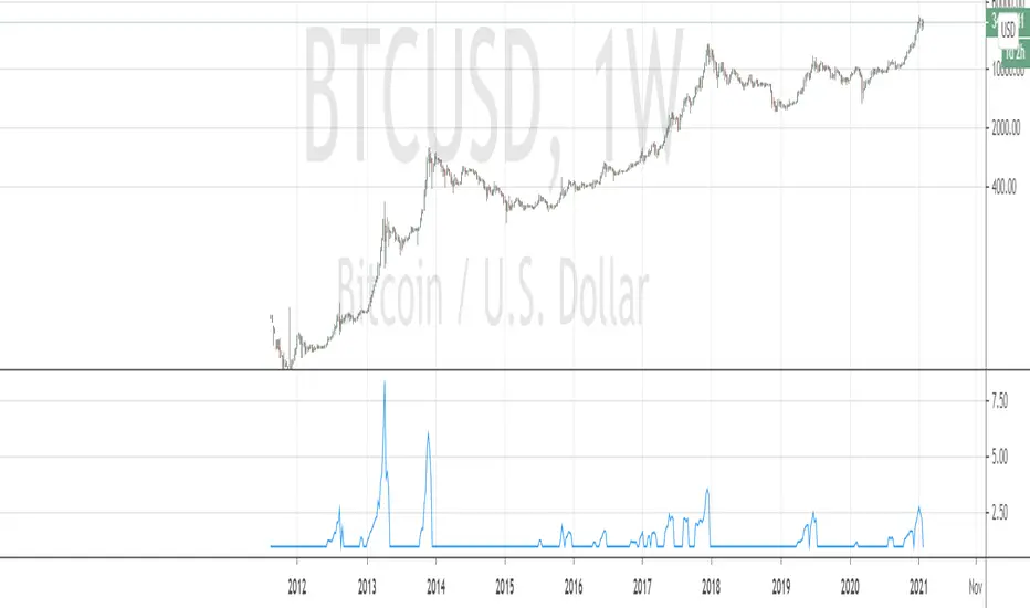
Bitcoin Bubble Strength IndexFor those who interested, here is a Bitcoin Strength Index source code. I used it on weekly chart with params (close,28). And only with Bitcoin . And only during bull run. It shows how far price went off the particular moving average during bubble run (i.e. being above BB). Weekly MA 28 is approximately daily ma 200.
The physical meaning of this indicator is to show current bull rally "speed".
Поиск скриптов по запросу "bitcoin"
Bitcoin Bullish Percent IndexHello Traders,
This is Bitcoin Bullish Percent Index script. First lets talk about what the Bullish Percent Index and how it is calculated:
"The Bullish Percent Index (BPI) is a breadth indicator based on the number of securities on Point & Figure Buy Signals, Developed by Abe Cohen in the mid-1950s. Because a security is either on a P&F Buy or Sell Signal, there is no ambiguity when it comes to P&F charts. This makes BPI a straightforward indicator with clearly defined signals."
The calculation is straightforward and simple: (Number of securities on P&F Buy signals) / (Total number of securities)
Here you can see what the P&F buy signal is:
In this script I choose 40 cryptos that is correlated ( as I see ) with BTC (including BtcUsdt). in the first part the script creates P&F chart for each security and check if there is Buy or Sell signal and sum the buy signals if there is. in the second part it creates P&F chart by using the P&F buy/sell signals coming from the securities P&F chart. because of complicated calculation the script may need a few seconds to load.
in the first part reversal value is 3 by default but you can set different values as reversal. sometimes I got better results with reversal = 5.
in BPI part reversal = 3 is used. so each box represents 2% (each X or O is a box). And this means it takes at least a 6% move in BPI for a reversal. the Bullish Percent Index favors the bulls when above 50% and the bears when below 50%. The bulls have the edge when over 50% of stocks are on a P&F Buy Signal. BPI is also considered overbought when above 70% and oversold when below 30%. BPI can move between 0 and 100.
Because of 40 securities are used in the script and all different prices, it uses Percentage scaling only. it can calculate the Percentage automatically by using the time frame of the chart or you can set it as you wish.
The Signals coming from BPI:
Bull Alert: BPI is below 30% and then forms a new column of X's (rises)
Bear Alert: BPI is above 70% and then forms a new column of O's that decline below 70%.
Bull Confirmed: BPI is on a P&F buy signal and in a column of X's (rising).
Bear Confirmed: BPI is on a P&F sell signal and in a column of O's (falling).
Bull Correction: BPI is on a P&F buy signal, but currently falling (column of O's).
Bear Correction: BPI is on a P&F sell signal, but currently rising (column of X's).
If you are not familiar with Bullish Percent Index you better search it on the net to get more info, you can find a lot of articles and web sites about BPI.
as I remember I developed the script 6-7 months ago and today I had chance to publish it as it was
Enjoy!

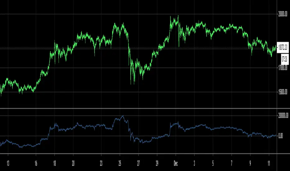
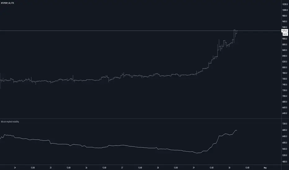
Bitcoin Implied VolatilityThis simple script collects data from FTX:BVOLUSD to plot BTC’s implied volatility as a standalone indicator instead of a chart.
Implied volatility is used to gauge future volatility and often used in options trading.
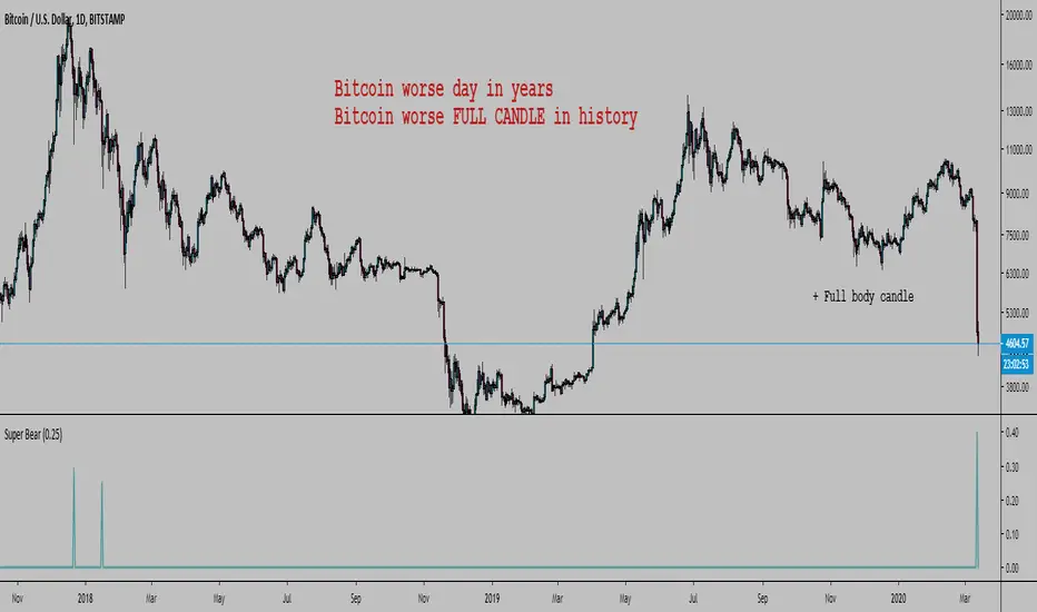
Bitcoin Worse DaysHello, here is a simple script to scan for BTC worse days.
In input you tell the script what are the minimum percent drops to look for.
By default it is 0.3, here I set it at 0.25 or it would not show anything except the 12 March (which is 40.07%).
The indicator has a precision of 1% I think.
It does not look at how low the body closed, it will show all days that closed below where they opened looking at how far below the high of the day the low was.
It can also work on any timeframe.
Here were the previous worse days from the late 2017 crash start of the bear market:
You could modify the script and look for the worse bodies with open - close instead of high - low
You could also add a filter to only look at days where the body is > 90% the whole candle (in this case it's got to be about 99%)
We can look back at BTC past a bit
Every bear market started with a large drop so we can expect...
As you can see we can look at the weekly chart too:
I won't lie, I am pretty happy. Russia, China bat eating community, and Greta were a big help. Thanks guys.

Bitcoin CME Gaps [NeoButane]Simple script that checks for gaps in price from CME. tickerid(x, y, sess) doesn't seem to be applying correctly for the ticker specified at the moment so there are a couple of 'gaps' peppered on lower timeframes.
Gaps are legitimate price levels to look as a support or resistance. The theory is that volume needs to be gap filled, but I currently believe it's an easy entry/exit trade for those who can move the market. I don't think there is sound analysis behind the why, but it is real.

Bitcoin Logarithmic Growth Curves & ZonesI found this awesome script from @quantadelic and edited it to be a bit more legible for regular use, including coloured zones and removing the intercept / slope values as variables, to leave space for the fib levels in the indicator display. I hope you all like it.

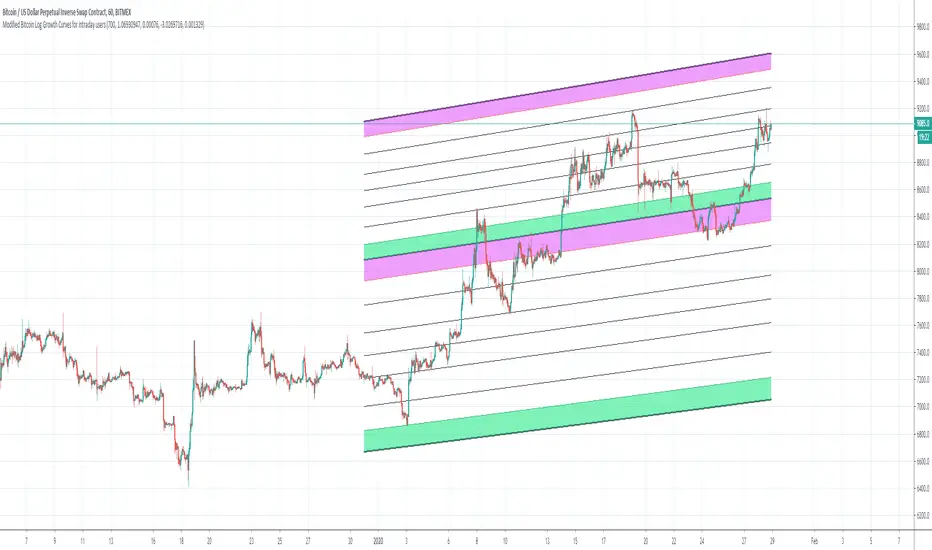
Bitcoin Logarithmic Growth Curves for intraday usersI wish to thank @Quantadelic who created this great indicator and leaving it open for others to improve.
I have made changes to make it user-friendly for the intraday traders.
The changes made have been;
1. Compartmentalized each area of the major Fibonacci level;
2. Added minor Fibonacci levels;
3. Color-coded the support and resistance levels, for better viewing;
4. Zoned each area of the major Fibonacci level; and
5. Created a time-frame display period for quicker loading of the indicator.
I have removed a few things to allow the indicator to run quicker;
1. Future projections; and
2. The major higher levels of the Fibonacci, which may be useful when Bitcoin reaches 100k.
Enjoy
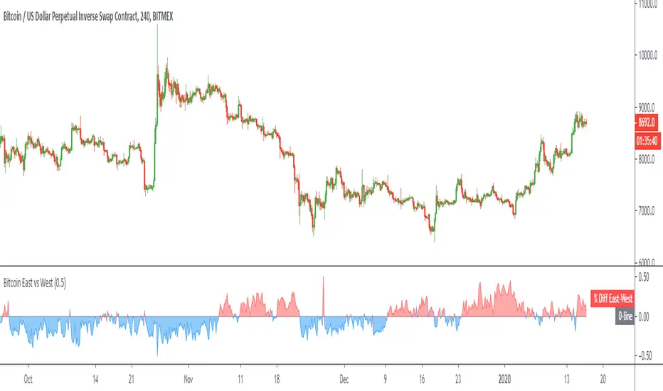
Bitcoin East vs WestPlots the volume weighted price difference between the top spot exchanges in the "East" (Asian markets) versus the "West" (US/UK/EU markets).
Optional: view the volume difference between the two.
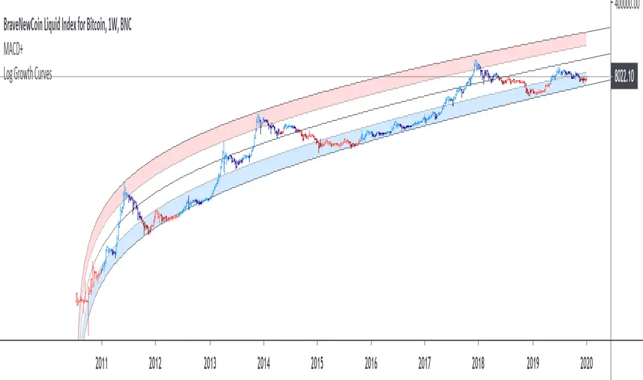
Bitcoin Logarithmic Growth CurvesThis is a version of the Log Growth Curves previously published by Quantadelic. The update includes customizable fib levels and filled upper and lower bands. This script is only intended for the Bitcoin log chart to reflect the channel that can be found on a log/log Bitcoin chart. The projections out from current levels are theoretical path of BTC based on the current trajectory.
In theory, reaching into the bottom zone of this chart is a good zone for accumulation while the top zone is a good are for distribution.
Bitcoin entry pointSimple script implementing lookintobitcoin dot com/charts/Bitcoin-Investor-Tool/
There are alerts available

Bitcoin Network Value to Transactions [aamonkey]Cryptoassets have been quite turbulent in the past few weeks.
At times like this, it is especially important to look at the fundamental foundations of cryptoassets.
This indicator is based on the Network Value to Transactions , or NVT .
Definition:
NVT = Network Value / Daily Transaction Volume
Because this indicator is pulling the Daily Transaction Volume for BTC it can only be used for BTC and the daily timeframe.

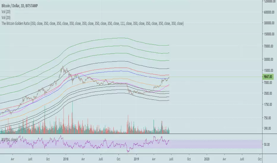
Bitcoin Golden RatioGives the top and bottom of the cryptocurrencies cycles.
When DMA111 crosses DMA350*2, the top is in.
Show accumulation phases and resistances with very precise accuracy.
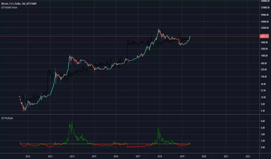
Bitcoin Stock to Flow Multiple (fixed)This is a fixed version of the original script by yomofoV:
I fixed the variable assignments and added switching of timeframes over indicator inputs.
To switch timeframes click on the indicator, open its settings and switch the timeframe to either monthly, weekly or daily.
Bitcoin Liquid Indexbravenewcoin.com
TV doesn't allow you to view the Bitcoin Liquid Index on lower time frames if you aren't a Premium subscriber >:(
I cheesed the system by recreating the formula that BNC uses. It isn't an exact replica, but very very close!
It can be slow to load due to the security( ) calls.
Default settings use the timeframe of the chart, however, you can set a custom timeframe if you wish.
Cheers
DasanC

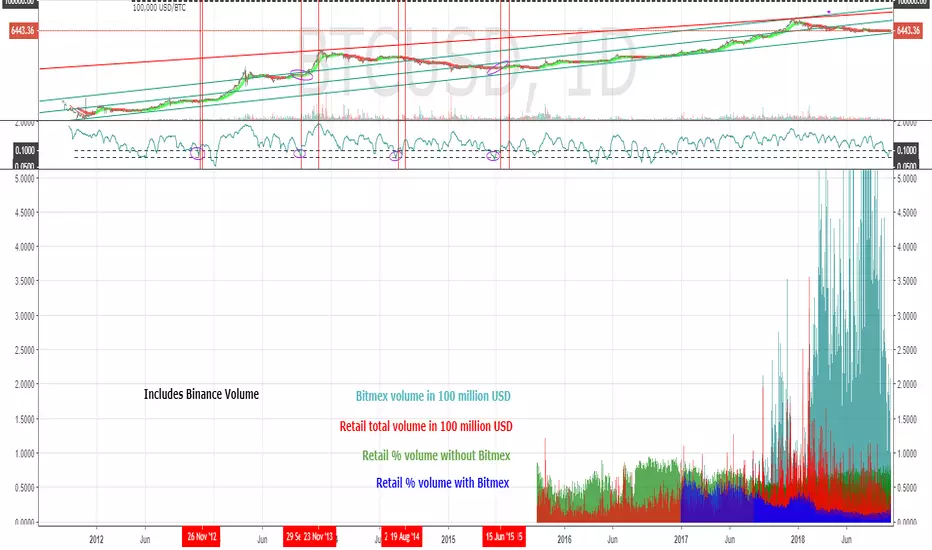
Bitcoin Retail Volume [jarederaj]Based on work published by @cryptorae
www.tradingview.com
Merges Binance volume into several metrics.
Bitcoin Shorts and LongsThis indicator shows the volume of shorts and longs for margin trading in Bitfinex.

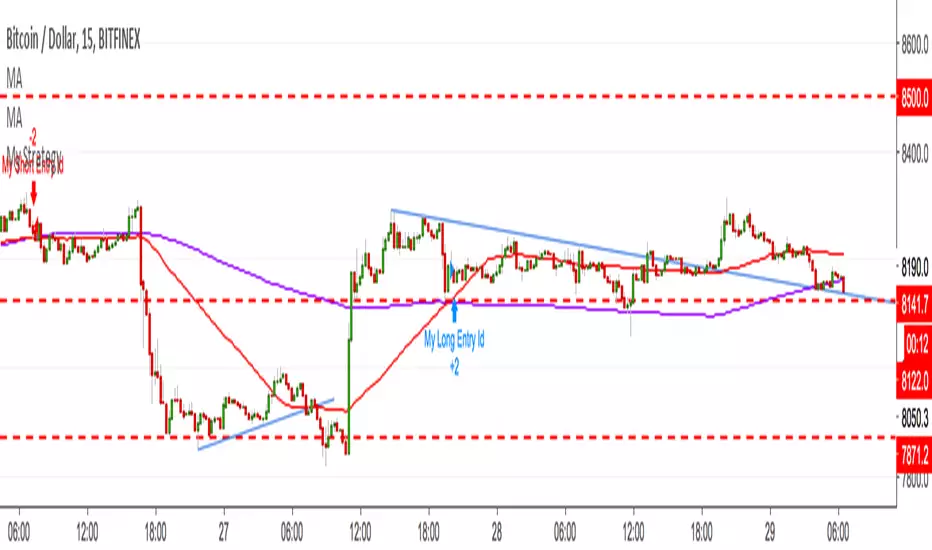
Bitcoin 15 min crossover SMA Strategy ScriptIs a very simple script that must be used on the 15 min chart of BTCUSD, and works.
Tested same EA in production since 2016.
Use the 200 and 50 SMA to buy and sell.
Works well!
Enjoi!
Bitcoin Kill Zones v2.1All I've changed in it from previous version is increased transparency. Makes it easier to observe now imo.

Bitcoin indexsDisplays average high and low, of the combined exchanges: Binance, Bittrex, Poloniex, Bitfinex, Bitmex, so that you can see arbitrage, and smooth out differences of exchanges for more realistic charting.
Sundays Suck for Bitcoin - Daily StrategyBitcoin tends to have bad Sundays, so this strategy just sells on Saturday, and buys back the next Wednesday if the price is kinda going up!
(Its Jonnys first script, so is this really just published for people looking for simple code to learn from :-)
(The strategy works best if you set your chart time period to 1 day.)
