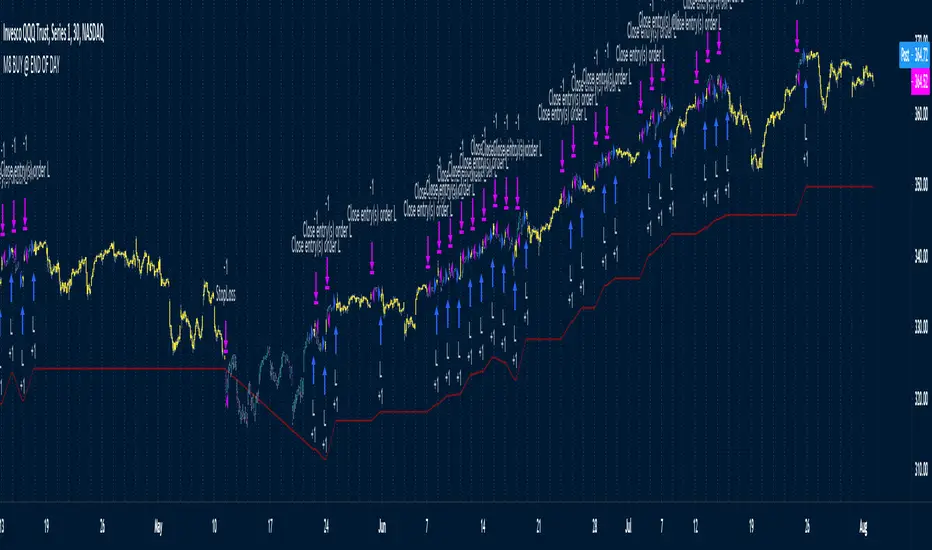
M8 BUY @ END OF DAYI've read a couple of times at a couple of different places that most of the move in the market happens after hours, meaning during non-standard trading hours.
After-market and pre-market hours and have seen data presented showing that systems which bought just before end normal market hours and sold the next morning had really amazing resutls.
But when testing those I found the results to be quite poor compared to the pretty graphs I saw, and after much tweaking and trying different ideas I gave up on the idea until I recently decided to try a new position management system.
The System
Buys at the end of the trading day before the close
Sells the next morning at the open IF THE CLOSE OF THE CURRENT BAR IS HIGHER THAN THE ENTRY PRICE
When the current price is not higher, the system will keep the position open until it EITHER gets stops out or closes on profit <<< this is WHY it has the high win %
The system has a high win ratio because it will keep that one position open until it either reaches profit or stops out
This "system" of waiting, and keeping the trade open, actually turned out to be a fantastic way to kind of put the complete trading strategy in a kind of limbo mode. It either waits for market failure or for a profit.
I don't really care about win % at all, almost always high win % ratio systems are just nonsense. What I look for is a PF -- profit factor of 1.5 or above, and a relatively smooth equity curve. -- This has both.
The Stop Loss setting is set @ .95, meaning a 5% stop loss. The Red Line on the chart is the stop loss line.
There is no set profit target -- it simply takes what the market gives.
Non-Repainting System
This does use a 200D Simple Moving Average as a filter. Like a Green Light / Red Light traffic light, the system will only trade long when the price is above its 200 Moving average.
Here is the code: "F1 = close > sma(security(syminfo.tickerid, "D", close ), MarketFilterLen) // HIGH OF OLD DATA -- SO NO REPAINTING"
I use "close ", so that's data from two days ago, it's fixed, confirmed, non-repainting data from the higher timeframe.
-- I would only suggest using this on direction tickers like SPY, QQQ, SSO, TQQQ, market sectors with additional filters in place.
Стратегия Pine Script®