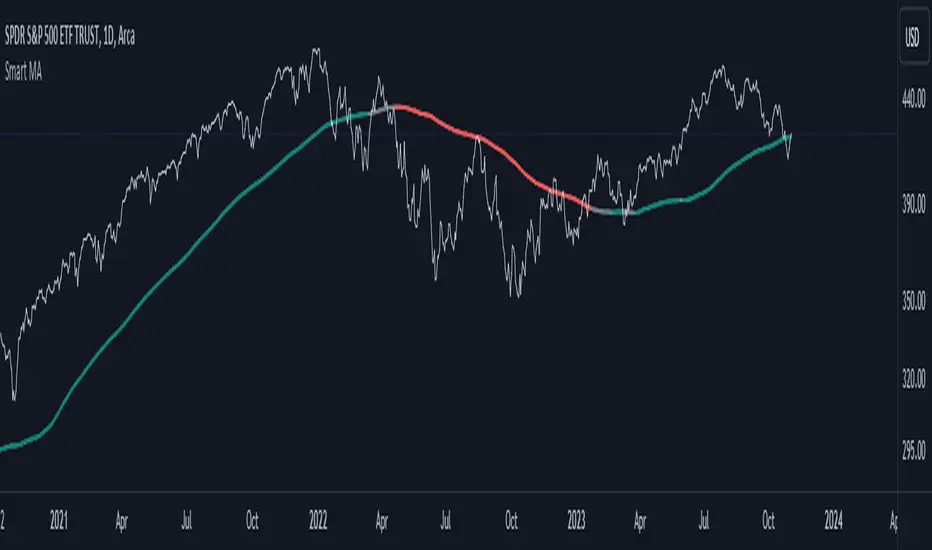
Smart MAThe Smart MA indicator is a tool designed for traders seeking insights into market trends, with its foundation rooted in moving averages. It offers two distinctive color options, with "Crossing" as the default choice and "Direction" as an alternative. Let's delve deeper into these options:
1. "Crossing" Color Option (Default):
Key Features:
Utilizes the interaction between fast and slow moving averages.
The color of the base moving average (MA) line dynamically changes based on crossovers between these moving averages.
Offers real-time visual signals for potential shifts in market sentiment.
Interpretation:
With the "Crossing" color option as the default setting, the base MA line's color responds to the interaction of the fast and slow moving averages.
A crossover where the fast MA crosses above the slow MA may prompt the base MA line to change to a bullish color (e.g., teal), indicating a potential bullish trend.
Conversely, if the fast MA crosses below the slow MA, the base MA line's color may alter to represent a bearish sentiment (e.g., red). This color shift provides a visual marker for a potential bearish trend, potentially guiding traders towards shorting opportunities.
2. "Direction" Color Option:
Key Features:
Focuses on the directional trend of the base moving average (MA).
The color of the base MA line signifies the direction in which the base MA is moving.
Aids in quickly identifying the prevailing market trend.
Interpretation:
Uptrend - Bullish Direction: When the base MA slopes upward, indicating an average price increase over the chosen base MA length, the base MA line's color may shift to a bullish hue (e.g., teal). This visual cue signals a potential uptrend, suggesting favorable long positions.
Downtrend - Bearish Direction: If the base MA slopes downward, signifying an average price decrease over the selected base MA length, the base MA line could change to a bearish shade (e.g., red). This color shift acts as an indicator of a potential downtrend, implying possible opportunities for shorting.
Customization:
Both color options allow traders to adjust the indicator's parameters, including base MA length, MA type, fast MA length, and slow MA length, to align with their trading strategies and preferred timeframes.
In summary, the Smart MA indicator, based on moving averages, provides traders with two color options: the default "Crossing" and "Direction" as an alternative. The "Crossing" option leverages fast and slow moving averages to offer real-time visual cues for dynamic market shifts. The "Direction" option simplifies trend analysis by focusing on the directional trend of the base MA. The choice between these options depends on your trading style and the depth of analysis you require. With the Smart MA indicator, you're equipped to make informed trading decisions in today's financial markets.
Поиск скриптов по запросу "deep股票代码"
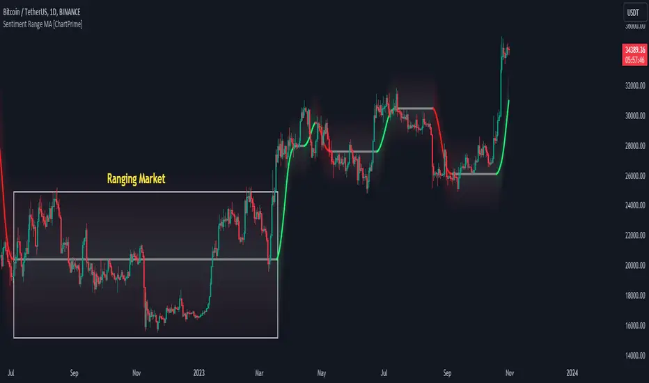
Sentiment Range MA [ChartPrime]The "Sentiment Range MA" provides traders with a dynamic perspective on market activity, emphasizing both stability in chop zones and quick adaptability outside of them.
Key Features:
Chop Zone Stability: In choppy markets, this indicator remains consistent, filtering out the noise to provide a clear view.
Quick Adaptability: Should the price break out of these zones, the indicator recalibrates promptly.
Dynamic Support and Resistance: Adapts based on the latest price action, serving as an evolving reference point.
Emphasis on Recent Levels: The tool factors in the latest notable market levels to stay relevant and timely.
Configurations:
Data Source: Choose your desired metric, though many default to the closing price.
Output Smoothing: Adjust the SR MA's response to market movements.
Trigger Smoothing: Refine boundary definitions based on your market insights.
ATR Period: Set the period for the ATR, influencing the surrounding boundary's width.
Range Multiplier: Control the ATR's effect on the range.
Range Switch: Flip between high-low and open-close values for range determination.
Visuals
Sentiment Range MA Line:
- This is the flowing line that transitions between green and red.
- When it's green, it indicates bullish momentum in the market. This suggests a prevailing upward trend and can be an entry cue for traders who trade with the trend.
- When it turns red, bearish sentiments dominate. It indicates the potential beginning of a downtrend or a continued downtrend. Traders might interpret this as a signal to be cautious, to short the market, or to exit long positions.
The Chop Zone:
- This is the space between the price candles and the Sentiment Range MA line. It represents a region where the price is considered to be moving sideways or without a clear direction. Price movements within the chop zone might not be substantial enough to warrant a trading decision. Only when the price breaks out of this zone do we see the Sentiment Range MA line change color, signaling a potential trading opportunity.
By interpreting these visuals, traders can make more informed decisions based on the prevailing market sentiment and trend. The chart becomes a tool, providing both an overview of the market condition and potential entry or exit points based on the Sentiment Range MA indicator's readings.
Detailed Settings Overview
Understanding the settings of the Sentiment Range MA Indicator can greatly enhance its utility in your trading strategy. Let's dive deeper into each:
Output Smoothing:
Purpose: It refines the SR MA to provide a clearer trend perspective.
Functionality:
- At `0`, it ensures the indicator responds immediately to price deviations from the chop zone.
- At higher values, it transforms the indicator into a volatility-adjusted moving average.
Filtering Modes:
- Single Filtering: Prioritizes speed.
- Double Filtering: Emphasizes stability.
Trigger Smoothing:
Purpose: Used for the range break detection.
Functionality: It dampens the indicator's sensitivity to sudden market volatility, preventing unnecessary triggers.
ATR Length:
Purpose: Governs the retrospective period for the chop zone.
Functionality:
- Higher values offer a more consistent and broad range size, capturing more historical data.
- Lower values allow for a more adaptive and responsive range.
Range Multiplier:
Purpose: Modifies the breadth of the range around the SR MA.
Functionality: Increasing the multiplier will extend the range, giving more leeway before triggering, while decreasing it will narrow the range, making the indicator more responsive to price changes.
Range Style:
Purpose: Decides which candlestick data is factored into the true range calculations.
Options:
- Body: Uses the open and close values.
- Wick: Accounts for the high and low values.
Functionality: Switching between styles lets you prioritize either the overall volatility (Wick) or just the concluded price action for a period (Body).
By fine-tuning these settings, traders can tailor the Sentiment Range MA Indicator to various market conditions and personal trading styles, ensuring optimal decision-making.
Quick Start
Based on the provided chart, here's a brief explanation of the default settings for the Sentiment Range MA Indicator:
Length: Set at ` 20 `.
- This determines the base moving average period. A standard setting, it calculates the average price over the last 20 periods, providing traders with a clear perspective of short-term trends.
ATR Length: Set at ` 200 `.
- This adjusts the lookback period for the Average True Range (ATR), which in turn influences the chop zone calculation. At a setting of 200, it offers a comprehensive view, considering a longer stretch of historical data.
Range Multiplier: Set at ` 6 `.
- This multiplies the ATR value, widening or narrowing the band around the SR MA. A setting of 6 means the range around the SR MA is determined by multiplying the ATR by 6, offering a broader fluctuation zone.
On the chart, the green line represents the bullish sentiment and the red represents the bearish sentiment. Price movements above and below these lines can be used as potential buy or sell signals respectively. Fine-tuning these settings can cater the Sentiment Range MA Indicator to your specific trading strategy and market condition preferences.
Alternative Settings
For traders looking to adapt to faster market conditions or prefer a more agile analysis, here's a brief description of the alternative settings for the Sentiment Range MA Indicator:
Length: Set at ` 3 `.
- This highly responsive setting calculates the average price over the last 3 periods. Ideal for quick market movements, it offers traders insights into very short-term price trends and potentially swift trade opportunities.
ATR Length: Set at ` 50 `.
- This shorter lookback period for the Average True Range (ATR) focuses on more recent market volatility, providing a tighter and more current chop zone calculation. It's suitable for those wanting to respond to recent market shifts.
Range Multiplier: Set at ` 4 `.
- Multiplying the ATR by 4 narrows down the buffer around the SR MA. This creates a tighter sentiment range, possibly resulting in more frequent crossovers and trading signals.
In the provided chart, the green line still denotes bullish momentum while the red symbolizes bearish sentiment. These alternative settings might generate more frequent signals, so traders should ensure their strategy is aligned with this heightened sensitivity.
Wrapping Up
The Sentiment Range MA melds stability and agility, making it a valuable tool in your trading toolkit. As always, before integrating new indicators, take the time to understand its nuances and potential impacts on your strategy.
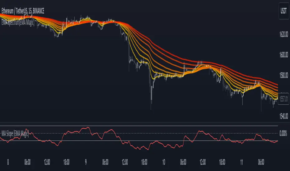
MA Slope [EMA Magic]█ Overview:
The MA Slope calculates the slope based on a given moving average.
The Moving Average Slope indicator allows you to identify the direction and the strength of a trend.
It calculates the rate of change in percentage based on the user-defined moving average.
█ Calculation: This indicator calculates the slope based on the changes of moving average and normalizes it with Average True Range(ATR).
The default value of ATR is 7.I recommend not changing it unless you know exactly what are you doing.
█ Input Settings:
The settings are divided into three sections:
The first section is for time frame adjustments. Modify it separately from the chart, Allows you to use moving averages from different time frames.
In the second section, you can configure the base calculation,including Moving Average and Average True Range(ATR) settings.
In the third section, you can detect breakout and sudden change signals, which are highlighted in the background of the indicator.
Note that When you change the breakout limit value, it also affects the band limit indicator on your chart.
To avoid signal confusion, use only one at a time.
Here is the example the breakout signals:
█ Usage:
When the slope is increasing, it indicates an uptrend.
When the slope is decreasing, it indicates a downtrend.
When the slope is moving around zero and choppy, it indicates no specific trend or price is in a range zone.
Uptrend and Range Zone example:
Downtrend example:
Slope peaks on extreme levels can signal a potential trend reversal point.
Breakout of the upper or lower bands can be translated into a trading signal.Indicating that price will probably continue to move in the direction of the breakout.
Favor long setups when the slope is increasing or it is positive and favor short setups when the slope is decreasing or it is negative.
Fits with any moving average you use, e.g., EMA, WMA, MA Ribbon, and more.
█ Alert
Alerts are available for both signal conditions.
█ Recap
Take the time to study price movements alongside this indicator for a deeper understanding.Whether you're a novice or experienced trader, this indicator can come helpful
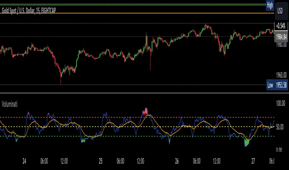
Voluminati: Uncovering Market SecretsVoluminati: Uncovering Market Secrets
Overview:
The Voluminati indicator dives deep into the secrets of trading volume, providing traders with unique insights into the market's strength and direction. This advanced tool visualizes the Relative Strength Index (RSI) of trading volume alongside the traditional RSI of price, presenting an enriched perspective on market dynamics.
Features:
Volume RSI: A unique twist on the traditional RSI, the Volume RSI measures the momentum of trading volume. This can help identify periods of increasing buying or selling pressure.
Traditional RSI: The renowned momentum oscillator that measures the speed and change of price movements. Useful for identifying overbought or oversold conditions.
Moving Averages: Both the Volume RSI and traditional RSI come with optional moving averages. These can be toggled on or off and are customizable in type (SMA or EMA) and length.
Overbought & Oversold Fills: Visual aids that highlight regions where the Volume RSI is in overbought (above 70) or oversold (below 30) territories. These fills help traders quickly identify potential reversal zones.
How to Use:
Look for divergence between the Volume RSI and price, which can indicate potential reversals.
When the Volume RSI moves above 70, it might indicate overbought conditions, and when it moves below 30, it might indicate oversold conditions.
The optional moving averages can be used to identify potential crossover signals or to smooth out the oscillators for a clearer trend view.
Customizations:
Toggle the display of the traditional RSI and its moving average.
Choose the type (SMA/EMA) and length for both the Volume RSI and traditional RSI moving averages.
Note: Like all indicators, the Voluminati is best used in conjunction with other tools and analysis techniques. Always use proper risk management.
RSI Heatmap Screener [ChartPrime]The RSI Heatmap Screener is a versatile trading indicator designed to provide traders and investors with a deep understanding of their selected assets' market dynamics. It offers several key features to facilitate informed decision-making:
█ Custom Asset Selection:
The user can choose up to 30 assets that you want to analyze, allowing for a tailored experience.
█ Adjustable RSI Length:
Customize your analysis by adjusting the RSI length to align with your trading strategy.
█ RSI Heatmap:
The heatmap feature uses various colors to represent RSI values:
█ Color coding for labels:
Grey: Signifies a neutral RSI, indicating a balanced market.
Yellow: Suggests overbought conditions, advising caution.
Pale Red: Indicates mild overbought conditions in a strong area.
Bright Red: Represents strong overbought conditions, hinting at a potential downturn.
Pale Green: Signals mild oversold conditions with signs of recovery.
Dark Green: Denotes full oversold conditions, with potential for a bounce.
Purple: Highlights extremely oversold conditions, pointing to an opportunity for a relief bounce.
█ Levels:
Central Plot and Zones: The central plot displays the average RSI of the selected assets, offering an overview of market sentiment. Overbought and oversold zones in red and green provide clear reference points.
█ Hover Labels:
Hover over an asset to access details on various indicators like VWAP, Stochastic, SMA, TradingView ranking, and Volume Rating. Bullish and bearish indicators are marked with ticks and crosses, and a fire emoji denotes heavily overextended assets.
█ TradingView Ranking:
Utilize the TradingView ranking metric to assess an asset's performance and popularity.
Thank you to @tradingview for this ranking metric.
█ Volume Rating:
Gain insights into trading volumes for more informed decision-making.
█ Oscillator at the Bottom:
The RSI average for the entire market, presented in a normalized format, offers a broader market perspective. Green indicates a favorable buying area, while red suggests market overextension and potential short or sell opportunities.
█ Heatmap Visualization:
Historical RSI values for each selected asset are displayed. Red indicates overbought conditions, while green signals oversold conditions, helping you spot trends and potential turning points.
This screener is designed to make entering the market simpler and more comprehensive for all traders and investors.

VWAP (Any Anchor)Hello Traders,
Introduction:
The Volume Weighted Average Price (VWAP) is a powerful trading indicator used to gauge the average price at which an asset has traded, weighted by volume, over a specific period.
One of the key factors that can significantly impact the effectiveness of VWAP is the concept of "anchoring." In this TradingView indicator script description, we'll explore the concept of anchoring and how it's integrated into a customizable VWAP indicator.
Understanding Anchoring:
Anchoring in VWAP refers to selecting a specific point in time from which the VWAP calculation begins.
This "anchor point" serves as the starting reference for VWAP, and it can substantially impact the indicator's behavior and interpretation.
Anchoring allows traders to adapt VWAP to different trading strategies and scenarios.
Here are some common anchor points used in the script and their significance:
1. Time-Based Anchors: Traders often anchor VWAP to specific times of the trading day, such as the market open (e.g., 9:30 am EST) or close (e.g., 4:00 pm EST).
You could add in the script any time-based anchor you think is relevant for your trading.
2. Event-Based Anchors: Anchoring can also be based on specific market events.
For example, some traders anchor VWAP to events like "3 Consecutive Green Candles" or "Supertrend" direction changes.
Feel free to adapt the script here and add the relevant events-based anchor for your trading.
3. Multi-Timeframe Anchoring: Traders can anchor VWAP on different timeframes, allowing them to analyze price and volume interactions across various horizons.
This flexibility is especially valuable for swing traders adapting to longer-term trends.
Anchor Selection
Traders can choose from various anchor points, including time-based, event-based, and even an "External Connector" for flexibility in adapting VWAP to specific scenarios.
The External connector is the output from another script used in this VWAP script.
Your script may have a condition being “true” whenever a signal is printed - you can use this signal as the anchor for the VWAP.
Conclusion:
Understanding anchoring in VWAP is essential for traders using this indicator effectively.
Choosing and customizing anchor points empowers traders to adapt VWAP to their specific trading styles and strategies.
Whether focused on intraday precision or analyzing longer-term trends, a customizable VWAP indicator with flexible anchoring options can be valuable to your trading toolkit.
Tailor your VWAP to your unique needs and gain deeper insights into market trends and price action.
Made with love
Dave

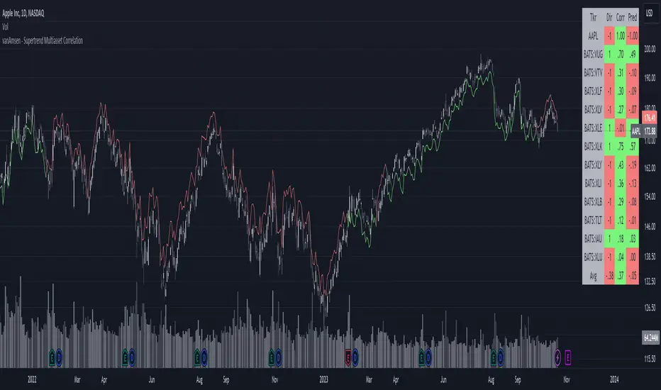
Supertrend Multiasset Correlation - vanAmsen Hello traders!
I am elated to introduce the "Supertrend Multiasset Correlation" , a groundbreaking fusion of the trusted Supertrend with multi-asset correlation insights. This approach offers traders a nuanced, multi-layered perspective of the market.
The Underlying Concept:
Ever pondered over the term Multiasset Correlation?
In the intricate tapestry of financial markets, assets do not operate in silos. Their movements are frequently intertwined, sometimes palpably so, and at other times more covertly. Understanding these correlations can unlock deeper insights into overarching market narratives and directional trends.
By melding the Supertrend with multi-asset correlations, we craft a holistic narrative. This allows traders to fathom not merely the trend of a lone asset but to appreciate its dynamics within a broader market tableau.
Strategy Insights:
At the core of this indicator is its strategic approach. For every asset, a signal is generated based on the Supertrend parameters you've configured. Subsequently, the correlation of daily price changes is assessed. The ultimate signal on the selected asset emerges from the average of the squared correlations, factoring in their direction. This indicator not only accounts for the asset under scrutiny (hence a correlation of 1) but also integrates 12 additional assets. By default, these span U.S. growth ETFs, value ETFs, sector ETFs, bonds, and gold.
Indicator Highlights:
The "Supertrend Multiasset Correlation" isn't your run-of-the-mill Supertrend adaptation. It's a bespoke concoction, tailored to arm traders with an all-encompassing view of market intricacies, fortified with robust correlation metrics.
Key Features:
- Supertrend Line : A crystal-clear visual depiction of the prevailing market trajectory.
- Multiasset Correlation : Delve into the intricate interplay of various assets and their correlation with your primary instrument.
- Interactive Correlation Table : Nestled at the top right, this table offers a succinct overview of correlation metrics.
- Predictive Insights : Leveraging correlations to proffer predictive pointers, adding another layer of conviction to your trades.
Usage Nuances:
- The bullish Supertrend line radiates in a rejuvenating green hue, indicative of potential upward swings.
- On the flip side, the bearish trajectory stands out in a striking red, signaling possible downtrends.
- A rich suite of customization tools ensures that the chart resonates with your trading ethos.
Parting Words:
While the "Supertrend Multiasset Correlation" bestows traders with a rejuvenated perspective, it's paramount to embed it within a comprehensive trading blueprint. This would include blending it with other technical tools and adhering to stringent risk management practices. And remember, before plunging into live trades, always backtest to fine-tune your strategies.
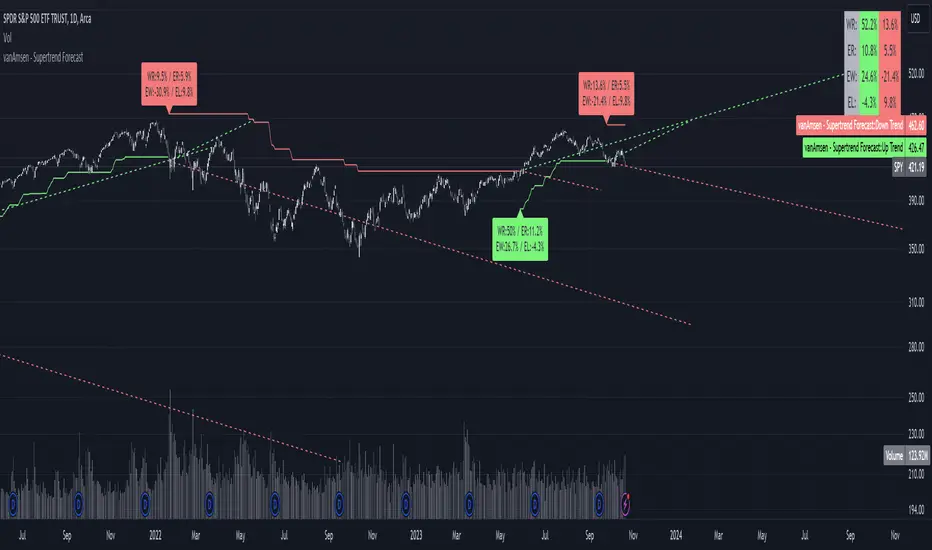
Supertrend Forecast - vanAmsenHello everyone!
I am thrilled to present the "vanAmsen - Supertrend Forecast", an advanced tool that marries the simplicity of the Supertrend with comprehensive statistical insights.
Before we dive into the functionalities of this indicator, it's essential to understand its foundation and theory.
The Theory:
What exactly is the Supertrend?
The Supertrend, at its core, is a momentum oscillator. It's a tool that provides buy and sell signals based on the prevailing market trend. The underlying principle is straightforward: by analyzing average price data and volatility over a period, the Supertrend gives us a line that represents the trend direction.
However, trading isn't just about identifying trends; it's about understanding their strength, potential profitability, and historical accuracy. This is where statistics come into play. By incorporating statistical analysis into the Supertrend, we can gain deeper insights into the market's behavior.
Description:
The "vanAmsen - Supertrend Forecast" isn't just another Supertrend indicator. It's a comprehensive tool designed to offer traders a holistic view of market trends, backed by robust statistical analysis.
Key Features:
- Supertrend Line: A visual representation of the current market direction.
- Win Rate & Expected Return: Delve into the historical accuracy and profitability of the prevailing trend.
- Average Percentage Change: Understand the average price fluctuation for both winning and losing trends.
- Forecast Lines: Project future price movements based on historical data, providing a roadmap for potential scenarios.
- Interactive Table: A concise table in the top right, offering a snapshot of all vital metrics at a glance.
Usage:
- The bullish Supertrend line adopts an Aqua hue, indicating potential upward momentum.
- In contrast, the bearish line is painted in Orange, suggesting potential downtrends.
- Customize your chart by toggling labels, tables, and lines according to preference.
Recommendation:
The "vanAmsen - Supertrend Forecast" is undoubtedly a powerful tool in a trader's arsenal. However, it's imperative to combine it with other technical analysis tools and sound risk management practices. It's always prudent to backtest strategies with historical data before embarking on live trading.
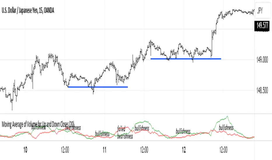
Moving Average of Volume for Up and Down ClosesThis indicator is intended to provide market bias information at a glance. Depending on the number of periods selected it can help identify changes in buying and selling sentiment or overall market bias. The two lines indicate increases and decreases in volumes for the selected number of periods. I recommend using this indicator with a minimum of clear support and resistance lines and a standard volume indicator. It does provided useful information as a stand-alone indicator. I don't use any indicators except volume, so this was meant to be my own personal volume analysis tool, however I feel that it can be very useful for other traders who may not have a deep understanding of volume analysis.
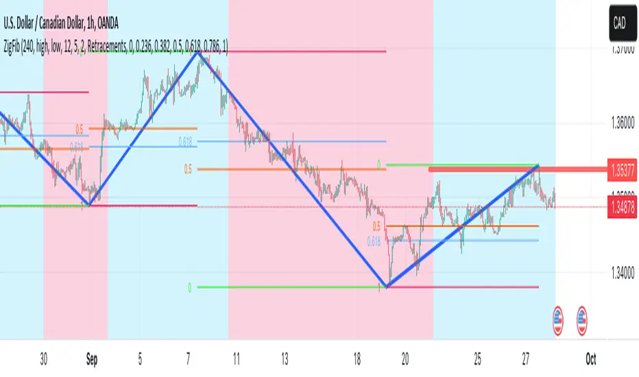
ZigZag++ FibonacciAuto Fibonacci tools are powerful ways designed to simplify your technical analysis by automatically drawing Fibonacci retracement and extension levels on your chart. This indicator is built to enhance your trading experience with clearer market moves and informative insights.
You can easily spot your waves and patterns when the percentages are moving with you.
Key Features:
Automated Fibonacci Levels: Plots Fibonacci retracement and extension levels based on recent price movements.
Multi-Timeframe Support: This indicator is your versatile companion, offering multi-timeframe functionality. You can seamlessly track Fibonacci levels across different resolutions, providing a comprehensive view of the market.
Two Types of Fibs: Retracement and Timeframe extension Fibonacci levels. Use retracements to identify potential reversal points and extensions to anticipate price targets, giving you a well-rounded perspective on market movements.
Benefits:
Save Time: No more manual Fibonacci drawing; It does this for you in real-time.
Enhanced Analysis: Gain a deeper understanding of potential support, resistance, and price targets.
User-Friendly: Suitable for traders of all levels, this indicator simplifies complex technical analysis.
For the math lovers
I started creating the ZigZag++ based on the MT4 calculation as I found it better performing than the tradingview inbuilt one. I have revised the calculation couple of times and now the final calculation is simple yet more accurate for my analysis.
First, I observe the market direction for the last Depth setting by comparing the rate at which high values reduce and low values increase. When the number of ticks set by Deviation is crossed and the last cross is more than the Backstep candles, then we have our ZigZag points.
These are the points we use in our Fibonacci calculation.
Checkout ZigLib below to use the same logic in your scripts.
Sample usage
This is a 4 Hour configuration with the default settings.
When the trend reversed, some key points I watch are 0.618 and 0.5. The market retraced back and formed the new point for the next ZigZag line on that level. This market behaviour happens quite often on these Fibonacci points. I would be looking for reversal or a break in this zone to know the next step.
Resources
ZigZag++ Lib by me; for retrieving the line points.
Fibonacci Toolkit by Lux Algo; For drawing the Timeframe Fibs. Very Amazing script.
PCA-Risk IndicatorOBJECTIVE:
The objective of this indicator is to synthesize, via PCA (Principal Component Analysis), several of the most used indicators with in order to simplify the reading of any asset on any timeframe.
It is based on my Bitcoin Risk Long Term indicator, and is the evolution of another indicator that I have not published 'Average Risk Indicator'.
The idea of this indicator is to use statistics, in this case the PCA, to reduce the number of dimensions (indicator) to aggregate them in some synthetic indicators (PCX)
I invite you to dig deeper into the PCA, but that is to try to keep as much information as possible from the raw data. The signal minus the noise.
I realized this indicator a year ago, but I publish it now because I do not see the interest to keep it private.
USAGE:
Unlike the Bitcoin Risk Long Term indicator, it does not make sense to change or disable the input indicators unless you use the 'Average Indicator' function. Because each input is weighted to generate the outputs, the PCX.
I extracted several courses (Bitcoin, Gold, S&P, CAC40) on several timeframes (W, D, 4h, 1h) of Trading view and use the Excel generated for the data on which I played the PCA analysis.
The results:
explained_variance_ratio: 0.55540809 / 0.13021972 / 0.07303142 / 0.03760925
explained_variance: 11.6639671 / 2.73470717 / 1.53371209 / 0.7898212
Interpretation:
Simply put, 55% of the information contained in each indicator can be represented with PC1, +13% with PC2, +7% with PC3, +3% with PC4.
What is important to understand is that PC1, which serves as a thermometer in a way, gives a simple indication of over-buying or over-selling area better than any other indicator.
PC2, difficult to interpret, is more reactive because precedes PC1, but can give false signals.
PC3 and PC4 do not seem relevant to me.
The way I use it is to take PC1 for Risk indicator, and display PC2 with 'Area'. When PC2 turns around and PC1 arrives on extremes, it can be good points to act.
NOTES :
- It is surprising that a simple average of all the indicators gives a fairly relevant result
- With Average indicator as Risk indicator, you can combine the indicators of your choice and see the predictive power with the staining of bars.
- You can add alerts on the levels of your choice on the Risk Indicator
- If you have any idea of adding an indicator, modification, criticism, bug found: share them, it’s appreciated!
---- FR ----
OBJECTIF :
L'objectif de cet indicateur est de synthétiser, via l'ACP (Analyse en Composantes Principales), plusieurs indicateurs parmi les plus utilisés avec afin de simplifier la lecture de n'importe quel actif sur n'importe quel timeframe.
Il est inspiré de mon indicateur 'Bitcoin Risk Long Term indicator', et est l'évolution d'un autre indicateur que je n'ai pas publié 'Average Risk Indicator'.
L'idée de cet indicateur est d'utiliser les statistiques, en l'occurence l'ACP, pour réduire le nombre de dimensions (indicateur) pour les agréger dans quelques indicateurs synthétiques (PCX)
Je vous invite à creuser l'ACP, mais c'est chercher à conserver un maximum d'informations à partir de la donnée brute. Le signal moins le bruit.
J'ai réalisé cet indicateur il y a un an, mais je le publie maintenant car je ne vois pas l'intérêt de le garder privé.
UTILISATION :
Contrairement à 'Bitcoin Risk Long Term indicator', il ne fait pas sens de modifier ou désactiver les indicateurs inputs, sauf si vous utiliser la fonction 'Average Indicator'. Car chaque input est pondéré pour générer les outputs, les PCX.
J'ai extrait plusieurs cours (Bitcoin, Gold, S&P, CAC40) sur plusieurs timeframes (W, D, 4h, 1h) de Trading view et utiliser les Excel généré pour la data sur laquelle j'ai joué l'analyse ACP.
Les résultats :
explained_variance_ratio : 0.55540809 / 0.13021972 / 0.07303142 / 0.03760925
explained_variance : 11.6639671 / 2.73470717 / 1.53371209 / 0.7898212
Interprétation :
Pour faire simple, 55% de l'information contenu dans chaque indicateur peut être représenté avec PC1, +13% avec PC2, +7% avec PC3, +3% avec PC4.
Ce qui faut y comprendre c'est que le PC1, qui sert de thermomètre en quelque sorte, donne une indication simple de zone de sur-achat ou sur-vente mieux que n'importe quel autre indicateur.
PC2, difficile à interpréter, est plus réactif car précède PC1, mais peut donner des faux signaux.
PC3 et PC4 ne me semble pas pertinent.
La manière dont je m'en sert c'est de prendre PC1 pour Risk indicator, et d'afficher PC2 avec 'Region'. Lorsque PC2 se retourne et que PC1 arrive sur des extrêmes, cela peut être des bons points pour agir.
NOTES :
- Il est étonnant de constater qu'une simple moyenne de tous les indicateurs donne un résultat assez pertinent
- Avec Average indicator comme Risk indicator, vous pouvez combiner les indicateurs de vos choix et voir la force prédictive avec la coloration des bars.
- Vous pouvez ajouter des alertes sur les niveaux de votre choix sur le Risk Indicator
- Si vous avez la moindre idée d'ajout d'indicateur, modification, critique, bug trouvé : partagez-les, c'est apprécié !

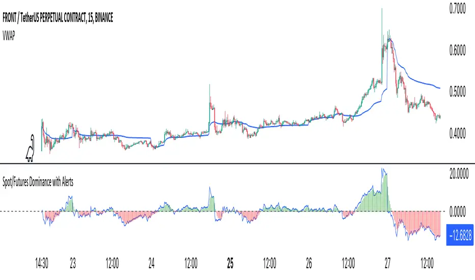
Crypto Spot/Futures Dominance Indicator with AlertsFutures/Spot Dominance Indicator:
Overview:
The futures/spot dominance indicator is a versatile tool used by traders and analysts to assess the relative strength or dominance of the futures market in relation to the spot (or cash) market for a specific asset. It offers insights into market sentiment, potential arbitrage opportunities, and risk management while incorporating the VWAP indicator for added context.
How It Works:
This indicator automatically detects and adapts to the futures symbol applied to the chart, simplifying the setup for traders. However, it still necessitates manual input of the corresponding spot pair to ensure accuracy.
Automatic Futures Symbol Detection: The indicator starts by automatically detecting the futures symbol on the trading chart, eliminating the need for manual configuration. This ensures that the indicator is applied to the correct futures contract.
Manual Spot Pair Entry: To provide a reliable reference point for the comparison, traders must manually input the corresponding spot symbol via the indicator's inputs. For instance, if the indicator detects the BTCUSDT.P futures symbol, traders would manually enter the BTCUSDT spot symbol.
Gathering Data: The indicator collects historical price data for both the detected futures contract and the manually specified spot symbol. This data includes open, high, low, and close prices, as well as trading volume.
VWAP Calculation: To gain a deeper understanding of price trends and market dynamics, the indicator calculates the VWAP (Volume Weighted Average Price) for both the futures and spot markets. The VWAP places more weight on prices with higher trading volume, offering a weighted average that reflects market consensus.
Premium/Discount Calculation: By subtracting the VWAP of the spot market from the VWAP of the futures market, the indicator quantifies the premium or discount of the futures price concerning the spot price. A positive value indicates a premium, while a negative value suggests a discount.
Plotting: The premium/discount value is displayed as a line on the chart, often alongside moving averages or other smoothing techniques for improved trend analysis.
Alerts: In addition to its analysis capabilities, this indicator now includes alerts to enhance your trading experience. It alerts you in the following scenarios:
Premium Above Average: Notifies you when the premium crosses above the average line.
Premium Below Average: Alerts you when the premium crosses below the average line.
Premium Above Zero: Provides an alert when the premium crosses above the zero line.
Premium Below Zero: Generates an alert when the premium crosses below the zero line.
Benefits of the Futures/Spot Dominance Indicator:
Sentiment Analysis: Traders use the indicator to assess market sentiment. A futures premium might signify bullish sentiment, while a discount could indicate bearish sentiment.
Arbitrage Opportunities: Identifying price discrepancies between futures and spot markets can help traders spot arbitrage opportunities, where they can profit from price differentials.
Risk Management: The indicator assists in evaluating risks associated with futures positions, helping traders manage their exposure effectively.
Trend Confirmation: When used in conjunction with other technical indicators, futures/spot dominance, along with VWAP, can provide additional confirmation of price trends.
Hedging: Investors and corporations use this tool to gauge the effectiveness of hedging strategies based on futures contracts.
Speculative Trading: Traders and investors use the indicator to inform speculative positions, aligning their trades with perceived market strength or weakness.
Insightful Analysis: Futures/spot dominance analysis, enriched by VWAP data, offers insights into market behavior during specific events or changes in economic conditions.
In summary, the futures/spot dominance indicator, with its integration of VWAP and automatic futures symbol detection, provides traders and investors with a comprehensive tool to assess market dynamics. It aids in sentiment analysis, risk management, and trend confirmation while offering potential arbitrage opportunities. The newly added alerts enhance the indicator's functionality, providing timely notifications of key market events. However, it relies on manual input of the corresponding spot pair to ensure precise comparisons between futures and spot markets. It should be used alongside other analysis techniques for a well-rounded view of the market.
Xeeder - Comparison RSI IndicatorXeeder - Comparison RSI Indicator (CRI)
The "Xeeder - Comparison RSI Indicator" (CRI) is a sophisticated tool designed to assist traders in analyzing and comparing the Relative Strength Index (RSI) and Moving Averages (MA) of two different securities simultaneously. This indicator is instrumental in identifying potential shifts in market momentum and strength between two assets.
Details of the Indicator:
Security Input Settings: This feature allows traders to input the symbols of two securities they wish to compare. The input is facilitated through text boxes where traders can enter the ticker symbols of their chosen securities.
Moving Average (MA) Settings: Traders have the option to select different types of moving averages such as SMA, EMA, WMA, among others. The settings also allow for the adjustment of the length of the moving average and the standard deviation multiplier for Bollinger Bands.
RSI Settings: This section allows traders to specify the length of the RSI calculation, which is used to analyze the momentum of the securities.
Dynamic RSI and MA Plotting: The indicator plots the RSI and its moving average for both securities dynamically on the chart, with distinct colors for easy differentiation and analysis.
RSI Bands: The indicator displays multiple RSI bands (Upper Band 1 & 2, Middle Band, Lower Band 1 & 2) as dashed horizontal lines, helping traders identify potential overbought and oversold regions.
Gradient Fill for Overbought and Oversold Regions: The indicator features a gradient fill between the RSI plot and the middle line, visually representing the overbought and oversold regions in different colors.
How to Use the Indicator:
Input Security Symbols: Start by entering the symbols of the two securities you wish to compare in the respective input boxes.
Configure MA and RSI Settings: Adjust the settings for the moving average type, length, and RSI length according to your trading strategy and analysis needs.
Analyze RSI and MA Plots: Observe the plotted RSI and moving averages for both securities to analyze and compare their momentum and trend characteristics.
Utilize RSI Bands: Use the RSI bands as reference points to identify potential overbought and oversold regions, and to gauge the relative strength between the two securities.
Interpret Gradient Fill: Pay attention to the gradient fill regions which visually represent overbought and oversold conditions, assisting in the identification of potential reversal points.
Example of Usage:
As a trader with a knack for developing innovative trading strategies, you can utilize the CRI indicator to enhance your swing trading approach. Here's how you might integrate this tool into your strategy:
Select Securities: Choose two securities that you are interested in comparing, perhaps from sectors you have identified as having potential based on your macroeconomic and geopolitical analysis.
Adjust Settings: Configure the RSI and MA settings to align with the characteristics of the selected securities and your trading strategy.
Analysis and Comparison: Analyze the RSI and MA plots to identify potential divergences or correlations between the two securities, which might indicate trading opportunities.
Utilize RSI Bands: Use the RSI bands to identify potential entry and exit points, aligning them with your analysis of broader market conditions and your trading strategy.
Content Creation: Leverage the insights gained from using the CRI indicator to create captivating content for your audience, sharing your analysis and perspectives on the selected securities and market conditions.
Remember, the CRI indicator serves as a powerful tool in your trading arsenal, offering a unique perspective on market dynamics and facilitating a deeper analysis of securities. Always consider the broader market context and your trading strategy when utilizing this tool.

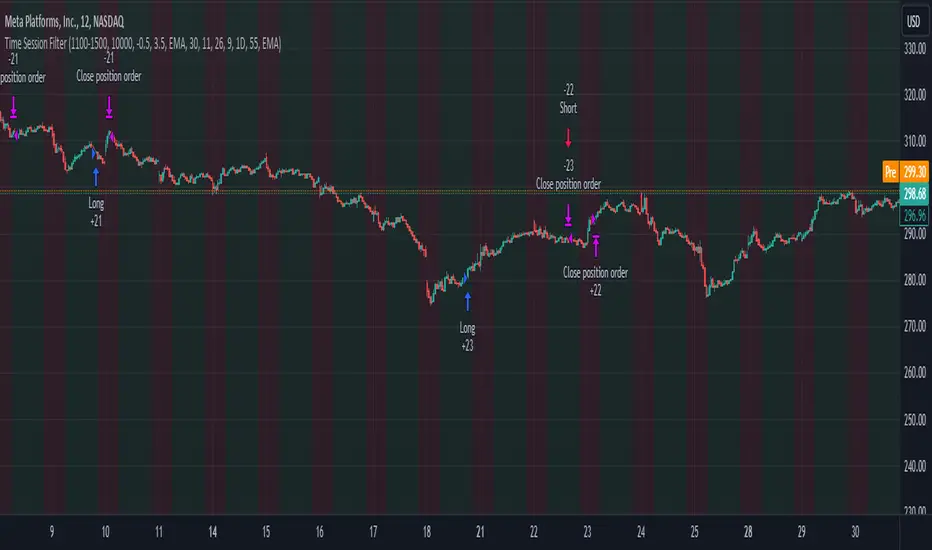
Time Session Filter - MACD exampleTime Session Filter in TradingView Strategy: A Comprehensive Guide
Welcome to this educational TradingView blog where we dive deep into the functionality and utility of the time session filter in trading strategies. It's interesting to note that the time session filter is a commonly overlooked feature in Pine Script, often not integrated into overall trading strategies. Yet, when used wisely, this tool can significantly enhance your trading approach. In essence, the session filter ensures that trades are only made within a specific, user-defined time frame. By incorporating this often-neglected building block, you can make your strategy more adaptable to various market conditions and trading preferences.
What is a Time Session Filter?
A time session filter is designed to:
Select Times of the Day to Trade: The filter allows you to choose specific hours during the day in which trades are allowed to be excecuted.
Toggle Days to Trade: You can decide which days of the week you want to trade, giving you the flexibility to avoid days that are historically not profitable for your strategy.
Close Trade When Session Ends: The filter can automatically close any open trade once the specified time session concludes, reducing the risk associated with holding positions outside your chosen time frame.
The user interface is streamlined, taking minimal space for the input sections, making it convenient to integrate with other indicators in your overall strategy script. In addition the script colors the background of the chart green when the timesession filter is on and makes the background red when the filter doesn't allow any trades. This helps you to visualise the selected timeframes in relation to chart patterns.
Best Practices for Time Selection
From my personal trading experience I share some input settings you can try to play around with:
Stocks: Trading stocks sometimes yield better results if you only trade in the mornings until lunchtime. This is the period when markets are generally more active, and traders are keenly participating.
Cryptocurrencies: For cryptocurrencies, it sometimes makes sense to avoid trading on Fridays, a day when futures contracts often expire. Various other market-moving events also typically occur on Fridays.
Random Selection: Interestingly, sometimes choosing a random selection of times and days can improve the script's performance, adding an element of unpredictability that might outperform more systematic approaches.
Strategy Overview
This strategy script incorporates various elements, including risk position size and MACD indicator, to provide a comprehensive trading strategy. For a detailed explanation of risk position sizing, please refer to this article:
For a complete understanding of the MACD indicator utilized, visit the following explanation:
Additionally, for high time frame trend filters, consult this resource for more info:
Educational Purposes and Risks
Please note that this script is for educational purposes and serves merely as an example of how to incorporate a time session filter into a trading strategy for pinescript. It is a simplified strategy without a fixed stop-loss, which can result in higher exposure to significant losses. The time session filter can be a powerful addition to your trading strategy, providing you with the tools to tailor your approach according to time-specific market conditions. By understanding its functionalities and best practices, you can make more informed trading decisions, but always remember that trading carries inherent risks.
Happy trading!
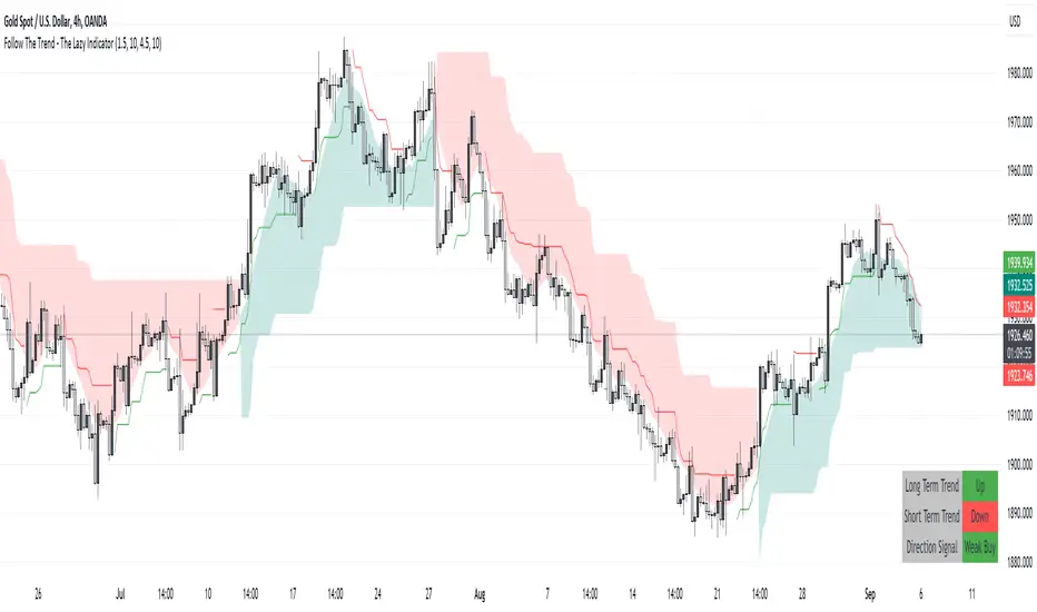
Follow The Trend - The Lazy Indicator**Understanding the 'Follow The Trend - The Lazy Indicator'**
This indicator is designed to help traders visualize the trend direction over both short-term and long-term periods. Let's dive deeper into understanding how it's designed and how it can be beneficial.
**1. How It's Designed:**
* **User Inputs:**
The first few lines ask the user for specific inputs related to the Average True Range (ATR) length and values for both short-term and long-term trends. ATR is a volatility indicator and, in this context, is used as part of the SuperTrend calculation.
* **SuperTrend Calculations:**
This indicator uses the SuperTrend, a popular trend-following indicator. Here, two SuperTrends are being calculated – one for short-term trends and another for long-term trends. The direction of the SuperTrend is also determined, signaling whether the trend is upwards or downwards.
* **Visual Representations:**
* The short-term SuperTrend is represented using green lines (for uptrend) and red lines (for downtrend).
* The indicator also provides a "cloud" between a Simple Moving Average (SMA) of the closing price (over the past 10 periods) and the long-term SuperTrend. This cloud changes color based on the direction of the long-term trend, providing another visual cue about market direction.
* **Signal Evaluation:**
This part of the code interprets the combination of short-term and long-term trends and assigns trading signals like "Strong Buy," "Weak Buy," "Strong Sell," "Weak Sell," and so on. This can act as a guide for traders, suggesting potential trading actions based on the prevailing trends.
* **Signal Coloration:**
The indicator also assigns colors to each signal. For instance, "Strong Buy" is green, "Strong Sell" is red, and there are transparency adjustments for weak signals to differentiate them from strong ones.
* **Tabular Presentation:**
At the end of the script, there’s a table displayed on the chart, summarizing the direction of both the long-term and short-term trends, as well as the overall trading signal. It provides a quick snapshot for traders to understand the current market scenario.
**2. How It May Be Helpful:**
* **Simplicity:**
The "Follow The Trend" indicator, despite its underlying complexity, is presented in a very user-friendly way. By just looking at the color cues and the table, traders can quickly understand the market's trend and potential direction.
* **Dual Trend Analysis:**
By analyzing both short-term and long-term trends, traders get a comprehensive view. This helps in understanding if the market is just having a short-term retracement (temporary reverse in direction) or if there's a genuine change in the long-term trend.
* **Adaptability:**
Traders can adjust the ATR values and lengths to customize the sensitivity of the indicator. This means it can be adapted to different assets or varying market conditions.
* **Actionable Signals:**
The signals like "Strong Buy" or "Weak Sell" are direct suggestions that can help in decision-making. Especially for beginners or those who might be overwhelmed by complex charts, such signals can be very beneficial.
* **Visual Appeal:**
The combination of trend lines, cloud coloring, and tabulated information provides a visually pleasing and easy-to-understand representation of market data. This can help reduce analysis fatigue and make chart reading more enjoyable.
In conclusion, the "Follow The Trend - The Lazy Indicator" is designed to make trend-following more accessible and actionable. By providing clear visual cues and combining short-term and long-term trend analysis, it offers traders a tool that's both comprehensive and user-friendly. Whether you're a beginner looking for clear signals or an experienced trader wanting an overview of the market trend, this indicator might be a useful addition to your toolkit.
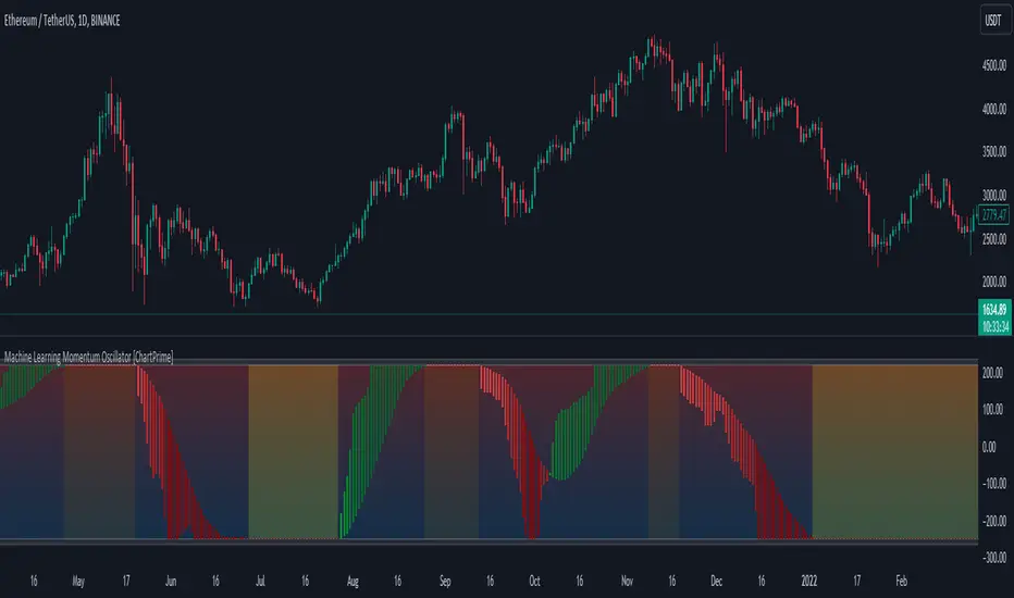
Machine Learning Momentum Oscillator [ChartPrime]The Machine Learning Momentum Oscillator brings together the K-Nearest Neighbors (KNN) algorithm and the predictive strength of the Tactical Sector Indicator (TSI) Momentum. This unique oscillator not only uses the insights from TSI Momentum but also taps into the power of machine learning therefore being designed to give traders a more comprehensive view of market momentum.
At its core, the Machine Learning Momentum Oscillator blends TSI Momentum with the capabilities of the KNN algorithm. Introducing KNN logic allows for better handling of noise in the data set. The TSI Momentum is known for understanding how strong trends are and which direction they're headed, and now, with the added layer of machine learning, we're able to offer a deeper perspective on market trends. This is a fairly classical when it comes to visuals and trading.
Green bars show the trader when the asset is in an uptrend. On the flip side, red bars mean things are heading down, signaling a bearish movement driven by selling pressure. These color cues make it easier to catch the sentiment and direction of the market in a glance.
Yellow boxes are also displayed by the oscillator. These boxes highlight potential turning points or peaks. When the market comes close to these points, they can provide a heads-up about the possibility of changes in momentum or even a trend reversal, helping a trader make informed choices quickly. These can be looked at as possible reversal areas simply put.
Settings:
Users can adjust the number of neighbours in the KNN algorithm and choose the periods they prefer for analysis. This way, the tool becomes a part of a trader's strategy, adapting to different market conditions as they see fit. Users can also adjust the smoothing used by the oscillator via the smoothing input.
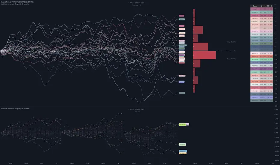
Multi-Asset Performance [Spaghetti] - By LeviathanThis indicator visualizes the cumulative percentage changes or returns of 30 symbols over a given period and offers a unique set of tools and data analytics for deeper insight into the performance of different assets.
Multi Asset Performance indicator (also called “Spaghetti”) makes it easy to monitor the changes in Price, Open Interest, and On Balance Volume across multiple assets simultaneously, distinguish assets that are overperforming or underperforming, observe the relative strength of different assets or currencies, use it as a tool for identifying mean reversion opportunities and even for constructing pairs trading strategies, detect "risk-on" or "risk-off" periods, evaluate statistical relationships between assets through metrics like correlation and beta, construct hedging strategies, trade rotations and much more.
Start by selecting a time period (e.g., 1 DAY) to set the interval for when data is reset. This will provide insight into how price, open interest, and on-balance volume change over your chosen period. In the settings, asset selection is fully customizable, allowing you to create three groups of up to 30 tickers each. These tickers can be displayed in a variety of styles and colors. Additional script settings offer a range of options, including smoothing values with a Simple Moving Average (SMA), highlighting the top or bottom performers, plotting the group mean, applying heatmap/gradient coloring, generating a table with calculations like beta, correlation, and RSI, creating a profile to show asset distribution around the mean, and much more.
One of the most important script tools is the screener table, which can display:
🔸 Percentage Change (Represents the return or the percentage increase or decrease in Price/OI/OBV over the current selected period)
🔸 Beta (Represents the sensitivity or responsiveness of asset's returns to the returns of a benchmark/mean. A beta of 1 means the asset moves in tandem with the market. A beta greater than 1 indicates the asset is more volatile than the market, while a beta less than 1 indicates the asset is less volatile. For example, a beta of 1.5 means the asset typically moves 150% as much as the benchmark. If the benchmark goes up 1%, the asset is expected to go up 1.5%, and vice versa.)
🔸 Correlation (Describes the strength and direction of a linear relationship between the asset and the mean. Correlation coefficients range from -1 to +1. A correlation of +1 means that two variables are perfectly positively correlated; as one goes up, the other will go up in exact proportion. A correlation of -1 means they are perfectly negatively correlated; as one goes up, the other will go down in exact proportion. A correlation of 0 means that there is no linear relationship between the variables. For example, a correlation of 0.5 between Asset A and Asset B would suggest that when Asset A moves, Asset B tends to move in the same direction, but not perfectly in tandem.)
🔸 RSI (Measures the speed and change of price movements and is used to identify overbought or oversold conditions of each asset. The RSI ranges from 0 to 100 and is typically used with a time period of 14. Generally, an RSI above 70 indicates that an asset may be overbought, while RSI below 30 signals that an asset may be oversold.)
⚙️ Settings Overview:
◽️ Period
Periodic inputs (e.g. daily, monthly, etc.) determine when the values are reset to zero and begin accumulating again until the period is over. This visualizes the net change in the data over each period. The input "Visible Range" is auto-adjustable as it starts the accumulation at the leftmost bar on your chart, displaying the net change in your chart's visible range. There's also the "Timestamp" option, which allows you to select a specific point in time from where the values are accumulated. The timestamp anchor can be dragged to a desired bar via Tradingview's interactive option. Timestamp is particularly useful when looking for outperformers/underperformers after a market-wide move. The input positioned next to the period selection determines the timeframe on which the data is based. It's best to leave it at default (Chart Timeframe) unless you want to check the higher timeframe structure of the data.
◽️ Data
The first input in this section determines the data that will be displayed. You can choose between Price, OI, and OBV. The second input lets you select which one out of the three asset groups should be displayed. The symbols in the asset group can be modified in the bottom section of the indicator settings.
◽️ Appearance
You can choose to plot the data in the form of lines, circles, areas, and columns. The colors can be selected by choosing one of the six pre-prepared color palettes.
◽️ Labeling
This input allows you to show/hide the labels and select their appearance and size. You can choose between Label (colored pointed label), Label and Line (colored pointed label with a line that connects it to the plot), or Text Label (colored text).
◽️ Smoothing
If selected, this option will smooth the values using a Simple Moving Average (SMA) with a custom length. This is used to reduce noise and improve the visibility of plotted data.
◽️ Highlight
If selected, this option will highlight the top and bottom N (custom number) plots, while shading the others. This makes the symbols with extreme values stand out from the rest.
◽️ Group Mean
This input allows you to select the data that will be considered as the group mean. You can choose between Group Average (the average value of all assets in the group) or First Ticker (the value of the ticker that is positioned first on the group's list). The mean is then used in calculations such as correlation (as the second variable) and beta (as a benchmark). You can also choose to plot the mean by clicking on the checkbox.
◽️ Profile
If selected, the script will generate a vertical volume profile-like display with 10 zones/nodes, visualizing the distribution of assets below and above the mean. This makes it easy to see how many or what percentage of assets are outperforming or underperforming the mean.
◽️ Gradient
If selected, this option will color the plots with a gradient based on the proximity of the value to the upper extreme, zero, and lower extreme.
◽️ Table
This section includes several settings for the table's appearance and the data displayed in it. The "Reference Length" input determines the number of bars back that are used for calculating correlation and beta, while "RSI Length" determines the length used for calculating the Relative Strength Index. You can choose the data that should be displayed in the table by using the checkboxes.
◽️ Asset Groups
This section allows you to modify the symbols that have been selected to be a part of the 3 asset groups. If you want to change a symbol, you can simply click on the field and type the ticker of another one. You can also show/hide a specific asset by using the checkbox next to the field.
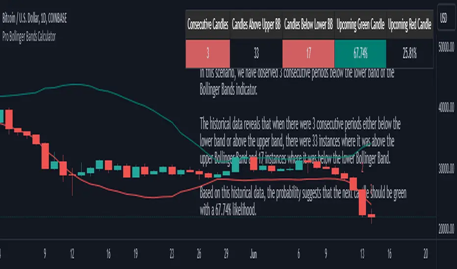
Pro Bollinger Bands CalculatorThe "Pro Bollinger Bands Calculator" indicator joins our suite of custom trading tools, which includes the "Pro Supertrend Calculator", the "Pro RSI Calculator" and the "Pro Momentum Calculator."
Expanding on this series, the "Pro Bollinger Bands Calculator" is tailored to offer traders deeper insights into market dynamics by harnessing the power of the Bollinger Bands indicator.
Its core mission remains unchanged: to scrutinize historical price data and provide informed predictions about future price movements, with a specific focus on detecting potential bullish (green) or bearish (red) candlestick patterns.
1. Bollinger Bands Calculation:
The indicator kicks off by computing the Bollinger Bands, a well-known volatility indicator. It calculates two pivotal Bollinger Bands parameters:
- Bollinger Bands Length: This parameter sets the lookback period for Bollinger Bands calculations.
- Bollinger Bands Deviation: It determines the deviation multiplier for the upper and lower bands, typically set at 2.0.
2. Visualizing Bollinger Bands:
The Bollinger Bands derived from the calculations are skillfully plotted on the price chart:
- Red Line: Represents the upper Bollinger Band during bearish trends, suggesting potential price declines.
- Teal Line: Represents the lower Bollinger Band in bullish market conditions, signaling the possibility of price increases.
3.Analyzing Consecutive Candlesticks:
The indicator's core functionality revolves around tracking consecutive candlestick patterns based on their relationship with the Bollinger Bands lines. To be considered for analysis, a candlestick must consistently close either above (green candles) or below (red candles) the Bollinger Bands lines for multiple consecutive periods.
4. Labeling and Enumeration:
To convey the count of consecutive candles displaying consistent trend behavior, the indicator meticulously assigns labels to the price chart. The position of these labels varies depending on the direction of the trend, appearing either below (for bullish patterns) or above (for bearish patterns) the candlesticks. The label colors match the candle colors: green labels for bullish candles and red labels for bearish ones.
5. Tabular Data Presentation:
The indicator complements its graphical analysis with a customizable table that prominently displays comprehensive statistical insights. Key data points within the table encompass:
- Consecutive Candles: The count of consecutive candles displaying consistent trend characteristics.
- Candles Above Upper BB: The number of candles closing above the upper Bollinger Band during the consecutive period.
- Candles Below Lower BB: The number of candles closing below the lower Bollinger Band during the consecutive period.
- Upcoming Green Candle: An estimated probability of the next candlestick being bullish, derived from historical data.
- Upcoming Red Candle: An estimated probability of the next candlestick being bearish, also based on historical data.
6. Custom Configuration:
To cater to diverse trading strategies and preferences, the indicator offers extensive customization options. Traders can fine-tune parameters such as Bollinger Bands length, upper and lower band deviations, label and table placement, and table size to align with their unique trading approaches.
Adjustable Bull Bear Candle Indicator (V1.2)Indicator Description: Adjustable Bull Bear Candle Indicator
This indicator, named "Adjustable Bull Bear Candle Indicator ," is designed to assist traders in identifying potential bullish and bearish signals within price charts. It combines candlestick pattern analysis, moving average crossovers, and RSI (Relative Strength Index) conditions to offer insights into potential trading opportunities.
Disclaimer:
Trading involves substantial risk and is not suitable for every investor. This indicator is a tool designed to aid in technical analysis, but it does not guarantee successful trades. Always exercise your own judgment and seek professional advice before making any trading decisions.
Key Features:
Preceding Candles Analysis:
The indicator examines the behavior of the previous 'n' candles to identify specific patterns that indicate bearish or bullish momentum.
Candlestick Pattern and Momentum:
It considers the relationship between the opening and closing prices of the current candle to determine if it's bullish or bearish. The indicator then assesses the absolute price difference and compares it to the cumulative absolute differences of preceding candles.
Moving Averages:
The indicator calculates two Simple Moving Averages (SMAs) – Close SMA and Far SMA – to help identify trends and crossovers in price movement.
Relative Strength Index (RSI):
RSI is used as an additional measure to gauge momentum. It analyzes the current price's magnitude of recent gains and losses and compares it to past data.
Time Constraint:
If enabled, the indicator operates within a specific time window defined by the user. This feature can help traders focus on specific market hours.
Customizable Alerts:
The indicator includes an alert system that can be enabled or disabled. You can also adjust the specific alert conditions to align with your trading strategy.
How to Use:
This indicator generates buy signals when specific conditions are met, including a bullish candlestick pattern, positive price difference, closing price above the SMAs, RSI above a threshold, preceding bearish candles, and optionally within a specified time window. Conversely, short signals are generated under conditions opposite to those of the buy signal.
Disclosure and Risk Warning:
Educational Tool: This indicator is meant for educational purposes and to aid traders in their technical analysis. It's not a trading strategy in itself.
Risk of Loss: Trading carries inherent risks, including the potential for substantial loss. Always manage risk and consider using proper risk management techniques.
Diversification: Do not rely solely on this indicator. A well-rounded trading approach includes fundamental analysis, risk management, and proper diversification.
Consultation: It's strongly advised to consult with a financial professional before making any trading decisions.
Conclusion:
The "Bullish Candle after Bearish Candles with Momentum Indicator" can be a valuable tool in your technical analysis toolkit. However, successful trading requires a deep understanding of market dynamics, risk management, and continual learning. Use this indicator in conjunction with other tools and strategies to enhance your trading decisions.
Remember that past performance is not indicative of future results. Always be cautious and informed when participating in the financial markets.
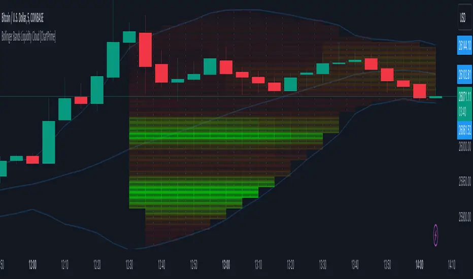
Bollinger Bands Liquidity Cloud [ChartPrime]This indicator overlays a heatmap on the price chart, providing a detailed representation of Bollinger bands' profile. It offers insights into the price's behavior relative to these bands. There are two visualization styles to choose from: the Volume Profile and the Z-Score method.
Features
Volume Profile: This method illustrates how the price interacts with the Bollinger bands based on the traded volume.
Z-Score: In this mode, the indicator samples the real distribution of Z-Scores within a specified window and rescales this distribution to the desired sample size. It then maps the distribution as a heatmap by calculating the corresponding price for each Z-Score sample and representing its weight via color and transparency.
Parameters
Length: The period for the simple moving average that forms the base for the Bollinger bands.
Multiplier: The number of standard deviations from the moving average to plot the upper and lower Bollinger bands.
Main:
Style: Choose between "Volume" and "Z-Score" visual styles.
Sample Size: The size of the bin. Affects the granularity of the heatmap.
Window Size: The lookback window for calculating the heatmap. When set to Z-Score, a value of `0` implies using all available data. It's advisable to either use `0` or the highest practical value when using the Z-Score method.
Lookback: The amount of historical data you want the heatmap to represent on the chart.
Smoothing: Implements sinc smoothing to the distribution. It smoothens out the heatmap to provide a clearer visual representation.
Heat Map Alpha: Controls the transparency of the heatmap. A higher value makes it more opaque, while a lower value makes it more transparent.
Weight Score Overlay: A toggle that, when enabled, displays a letter score (`S`, `A`, `B`, `C`, `D`) inside the heatmap boxes, based on the weight of each data point. The scoring system categorizes each weight into one of these letters using the provided percentile ranks and the median.
Color
Color: Color for high values.
Standard Deviation Color: Color to represent the standard deviation on the Bollinger bands.
Text Color: Determines the color of the letter score inside the heatmap boxes. Adjusting this parameter ensures that the score is visible against the heatmap color.
Usage
Once this indicator is applied to your chart, the heatmap will be overlaid on the price chart, providing a visual representation of the price's behavior in relation to the Bollinger bands. The intensity of the heatmap is directly tied to the price action's intensity, defined by your chosen parameters.
When employing the Volume Profile style, a brighter and more intense area on the heatmap indicates a higher trading volume within that specific price range. On the other hand, if you opt for the Z-Score method, the intensity of the heatmap reflects the Z-Score distribution. Here, a stronger intensity is synonymous with a more frequent occurrence of a specific Z-Score.
For those seeking an added layer of granularity, there's the "Weight Score Overlay" feature. When activated, each box in your heatmap will sport a letter score, ranging from `S` to `D`. This score categorizes the weight of each data point, offering a concise breakdown:
- `S`: Data points with a weight of 1.
- `A`: Weights below 1 but greater than or equal to the 75th percentile rank.
- `B`: Weights under the 75th percentile but at or above the median.
- `C`: Weights beneath the median but surpassing the 25th percentile rank.
- `D`: All that fall below the 25th percentile rank.
This scoring feature augments the heatmap's visual data, facilitating a quicker interpretation of the weight distribution across the dataset.
Further Explanations
Volume Profile
A volume profile is a tool used by traders to visualize the amount of trading volume occurring at specific price levels. This kind of profile provides a deep insight into the market's structure and helps traders identify key areas of support and resistance, based on where the most trading activity took place. The concept behind the volume profile is that the amount of volume at each price level can indicate the potential importance of that price.
In this indicator:
- The volume profile mode creates a visual representation by sampling trading volumes across price levels.
- The representation displays the balance between bullish and bearish volumes at each level, which is further differentiated using a color gradient from `low_color` to `high_color`.
- The volume profile becomes more refined with sinc smoothing, helping to produce a smoother distribution of volumes.
Z-Score and Distribution Resampling
Z-Score, in the context of trading, represents the number of standard deviations a data point (e.g., closing price) is from the mean (average). It’s a measure of how unusual or typical a particular data point is in relation to all the data. In simpler terms, a high Z-Score indicates that the data point is far away from the mean, while a low Z-Score suggests it's close to the mean.
The unique feature of this indicator is that it samples the real distribution of z-scores within a window and then resamples this distribution to fit the desired sample size. This process is termed as "resampling in the context of distribution sampling" . Resampling provides a way to reconstruct and potentially simplify the original distribution of z-scores, making it easier for traders to interpret.
In this indicator:
- Each Z-Score corresponds to a price value on the chart.
- The resampled distribution is then used to display the heatmap, with each Z-Score related price level getting a heatmap box. The weight (or importance) of each box is represented as a combination of color and transparency.
How to Interpret the Z-Score Distribution Visualization:
When interpreting the Z-Score distribution through color and alpha in the visualization, it's vital to understand that you're seeing a representation of how unusual or typical certain data points are without directly viewing the numerical Z-Score values. Here's how you can interpret it:
Intensity of Color: This often corresponds to the distance a particular data point is from the mean.
Lighter shades (closer to `low_color`) typically indicate data points that are more extreme, suggesting overbought or oversold conditions. These could signify potential reversals or significant deviations from the norm.
Darker shades (closer to `high_color`) represent data points closer to the mean, suggesting that the price is relatively typical compared to the historical data within the given window.
Alpha (Transparency): The degree of transparency can indicate the significance or confidence of the observed deviation. More opaque boxes might suggest a stronger or more reliable deviation from the mean, implying that the observed behavior is less likely to be a random occurrence.
More transparent boxes could denote less certainty or a weaker deviation, meaning that the observed price behavior might not be as noteworthy.
- Combining Color and Alpha: By observing both the intensity of color and the level of transparency, you get a richer understanding. For example:
- A light, opaque box could suggest a strong, significant deviation from the mean, potentially signaling an overbought or oversold scenario.
- A dark, transparent box might indicate a weak, insignificant deviation, suggesting the price is behaving typically and is close to its average.
CE - 42MACRO Fixed Income and Macro This is Part 2 of 2 from the 42MACRO Recreation Series
However, there will be a bonus Indicator coming soon!
The CE - 42MACRO Fixed Income and Macro Table is a next level Macroeconomic and market analysis indicator.
It aims to provide a probabilistic insight into the market realized GRID Macro regimes,
track a multiplex of important Assets, Indices, Bonds and ETF's to derive extra market insights by showing the most important aggregates and their performance over multiple timeframes... and what that might mean for the whole market direction.
For traders and especially investors, the unique functionalities will be of high value.
Quick guide on how to use it:
docs.google.com
WARNING
By the nature of the macro regimes, the outcomes are more accurate over longer Chart Timeframes (Week to Months).
However, it is also a valuable tool to form an advanced,
market realized, short to medium term bias.
NOTE
This Indicator is intended to be used alongside the 1nd part "CE - 42MACRO Equity Factor"
for a more wholistic approach and higher accuracy.
Methodology:
The Equity Factor Table tracks specifically chosen Assets to identify their performance and add the combined performances together to visualize 42MACRO's GRID Equity Model.
For this it uses the below Assets:
Convertibles ( AMEX:CWB )
Leveraged Loans ( AMEX:BKLN )
High Yield Credit ( AMEX:HYG )
Preferreds ( NASDAQ:PFF )
Emerging Market US$ Bonds ( NASDAQ:EMB )
Long Bond ( NASDAQ:TLT )
5-10yr Treasurys ( NASDAQ:IEF )
5-10yr TIPS ( AMEX:TIP )
0-5yr TIPS ( AMEX:STIP )
EM Local Currency Bonds ( AMEX:EMLC )
BDCs ( AMEX:BIZD )
Barclays Agg ( AMEX:AGG )
Investment Grade Credit ( AMEX:LQD )
MBS ( NASDAQ:MBB )
1-3yr Treasurys ( NASDAQ:SHY )
Bitcoin ( AMEX:BITO )
Industrial Metals ( AMEX:DBB )
Commodities ( AMEX:DBC )
Gold ( AMEX:GLD )
Equity Volatility ( AMEX:VIXM )
Interest Rate Volatility ( AMEX:PFIX )
Energy ( AMEX:USO )
Precious Metals ( AMEX:DBP )
Agriculture ( AMEX:DBA )
US Dollar ( AMEX:UUP )
Inverse US Dollar ( AMEX:UDN )
Functionalities:
Fixed Income and Macro Table
Shows relative market Asset performance
Comes with different Calculation options like RoC,
Sharpe ratio, Sortino ratio, Omega ratio and Normalization
Allows for advanced market (health) performance
Provides the calculated, realized GRID market regimes
Informs about "Risk ON" and "Risk OFF" market states
Visuals - for your best experience only use one (+ BarColoring) at a time:
You can visualize all important metrics:
- GRID regimes of the currently chosen calculation type
- Risk On/Risk Off with background colouring and additional +1/-1 values
- a smoother GRID model
- a smoother Risk On/ Risk Off metric
- Barcoloring for enabled metric of the above
If you have more suggestions, please write me
Fixed Income and Macro:
The visualisation of the relative performance of the different assets provides valuable information about the current market environment and the actual market performance.
It furthermore makes it possible to obtain a deeper understanding of how the interconnected market works and makes it simple to identify the actual market direction,
thus also providing all the information to derive overall market health, market strength or weakness.
Utility:
The Fixed Income and Macro Table is divided in 4 Columns which are the GRID regimes:
Economic Growth:
Goldilocks
Reflation
Economic Contraction:
Inflation
Deflation
Top 5 Fixed Income/ Macro Factors:
Are the values green for a specific Column?
If so then the market reflects the corresponding GRID behavior.
Bottom 5 Fixed Income/ Macro Factors:
Are the values red for a specific Column?
If so then the market reflects the corresponding GRID behavior.
So if we have Goldilocks as current regime we would see green values in the Top 5 Goldilocks Cells and red values in the Bottom 5 Goldilocks Cells.
You will find that Reflation will look similar, as it is also a sign of Economic Growth.
Same is the case for the two Contraction regimes.
******
This Indicator again is based to a majority on 42MACRO's models.
I only brought them into TV and added things on top of it.
If you have questions or need a more in-depth guide DM me.
GM

CE - 42MACRO Equity Factor Table This is Part 1 of 2 from the 42MACRO Recreation Series
The CE - 42MACRO Equity Factor Table is a whole toolbox packaged in a single indicator.
It aims to provide a probabilistic insight into the market realized GRID Macro Regime, use a multiplex of important Assets and Indices to form a high probability Implied Correlation expectation and allows to derive extra market insights by showing the most important aggregates and their performance over multiple timeframes... and what that might mean for the whole market direction, as well as the underlying asset.
WARNING
By the nature of the macro regimes, the outcomes are more accurate over longer Chart Timeframes (Week to Months).
However, it is also a valuable tool to form a proper,
market realized, short to medium term bias.
NOTE
This Indicator is intended to be used alongside the 2nd part "CE - 42MACRO Yield and Macro"
for a more wholistic approach and higher accuracy.
Due to coding limitations they can not be merged into one Indicator.
Methodology:
The Equity Factor Table tracks specifically chosen Assets to identify their performance and add the combined performances together to visualize 42MACRO's GRID Equity Model.
For this it uses the below Assets, with more to come:
Dividend Compounders ( AMEX:SPHD )
Mid Caps ( AMEX:VO )
Emerging Markets ( AMEX:EEM )
Small Caps ( AMEX:IWM )
Mega Cap Growth ( NASDAQ:QQQ )
Brazil ( AMEX:EWZ )
United Kingdom ( AMEX:EWU )
Growth ( AMEX:IWF )
United States ( AMEX:SPY )
Japan ( AMEX:DXJ )
Momentum ( AMEX:MTUM )
China ( AMEX:FXI )
Low Beta ( AMEX:SPLV )
International ex-US ( NASDAQ:ACWX )
India ( AMEX:INDA )
Eurozone ( AMEX:EZU )
Quality ( AMEX:QUAL )
Size ( AMEX:OEF )
Functionalities:
1. Correlations
Takes a measure of Cross Market Correlations
2. Implied Trend
Calculates the trend for each Asset and uses the Correlation to obtain the Implied Trend for the underlying Asset
There are multiple functionalities to enhance Signal Speed and precision...
Reading a signal only over a certain threshold, otherwise being colored in gray to signal noise or unclear market behavior
Normalization of Signal
Double Normalization of Signal for more Speed... ideal for the Crypto Market
Using an additional Hull Moving Average to enhance Signal Speed
Additional simple Background coloring to get a Signal from the HMA
Barcoloring based on the Implied Correlation
3. Equity Factor Table
Shows market realized Asset performance
Provides the approximate realized GRID market regimes
Informs about "Risk ON" and "Risk OFF" market states
Now into the juicy stuff...
Visuals:
There is a variety of options to change visual settings of what is plotted and where
+ additional considerations.
Everything that is relevant in the underlying logic which can improve comprehension can be visualized with these options.
More to come
Market Correlation:
The Market Correlation Table takes the Correlation of all the Assets to the Asset on the Chart,
it furthermore uses the Normalized KAMA Oscillator by IkkeOmar to analyse the current trend of every single Asset.
(To enhance the Signal you can apply the mentioned Indicator on the relevant Assets to find your target Asset movements that you intend to capture...
and then change the length of the Indicator in here)
It then Implies a Correlation based on the Trend and the Correlation to give a probabilistically adjusted expectation for the future Chart Asset Movement.
This is strengthened by taking the average of all Implied Trends.
Thus the Correlation Table provides valuable insights about probabilistically likely Movement of the Asset over the defined time duration,
providing alpha for Traders and Investors alike.
Equity Factors:
The table provides valuable information about the current market environment (whether it's risk on or risk off),
the rough GRID models from 42MACRO and the actual market performance.
This allows you to obtain a deeper understanding of how the market works and makes it simple to identify the actual market direction,
makes it possible to derive overall market Health and shows market strength or weakness.
Utility:
The Equity Factor Table is divided in 4 Sections which are the GRID regimes:
Economic Growth:
Goldilocks
Reflation
Economic Contraction:
Inflation
Deflation
Top 5 Equity Factors:
Are the values green for a specific Column?
If so then the market reflects the corresponding GRID behavior.
Bottom 5 Equity Factors:
Are the values red for a specific Column?
If so then the market reflects the corresponding GRID behavior.
So if we have Goldilocks as current regime we would see green values in the Top 5 Goldilocks Cells and red values in the Bottom 5 Goldilocks Cells.
You will find that Reflation will look similar, as it is also a sign of Economic Growth.
Same is the case for the two Contraction regimes.
This whole Indicator, as well as the second part, is based to a majority on 42MACRO's models.
I only brought them into TV and added things on top of it.
If you have questions or need a more in-depth guide DM me.
Will make a guide to all functionalities if necessity becomes apparent.
GM

Consolidation Spotter Multi Time FrameThis tool is designed for traders looking to spot areas of consolidation on their charts across various time frames. It highlights these consolidation areas using visually appealing boxes, making it easier to identify potential breakout or breakdown zones.
How To Use:
Spotting Consolidation: When you see a box form on your chart, this represents a consolidation zone. Within this zone, the price is moving sideways without a strong upward or downward trend.
Anticipating Breakouts & Breakdowns: Watch the price as it approaches the edges of the box. A movement outside the box can signal a potential breakout (if above the box) or a breakdown (if below the box). This is where momentum shifts can happen.
Momentum Confirmation: Once the price clearly moves out of the box, it indicates a momentum shift. If the price moves upwards out of the box, this can be seen as bullish momentum. Conversely, if the price moves downwards out of the box, this can be seen as bearish momentum.
To use the tool effectively, adjust the settings to suit your trading style, choose your preferred visual theme, and watch as the script highlights key consolidation areas on your chart.
Tip: To visualize fractals, consider using multiple instances of the "Consolidation Spotter" indicator, each set to a different timeframe. This approach allows you to observe consolidations nested within larger consolidations, offering deeper insights into market structures. 😉