Relative Strength Index (RSI) w/ Multi Time Frame w/ DivergencesThis indicator is an advanced evolution of the classic Relative Strength Index (RSI), designed to provide deeper market context by combining Momentum, Multi-Timeframe (MTF) analysis, and Divergences into a single, clean visual tool.
Unlike standard indicators, RSI MTF Pro v2 allows you to configure the Main RSI and the Background Trend Zone independently, giving you full control over your strategy (e.g., watching a 15m RSI while monitoring the 4H trend).
Key Features:
🚀 Dual MTF Engine: Completely independent settings for the Main RSI Line and the Background Zone. You can choose different Timeframes, Lengths, and Levels for each.
heatmap Style Background: The indicator background changes color (Red/Green) based on the MTF RSI trend, helping you filter out bad trades and stick to the dominant trend.
🎨 Smart Gradient Fills: To keep your chart clean, the gradient colors (Red/Green fills) only appear when the RSI breaches the Overbought or Oversold levels.
🎯 Divergence Detector: Automatically spots and marks Regular Bullish and Bearish divergences with pivot-based logic.
How to Use:
Trend Confirmation: Use the Background Color to determine the higher timeframe direction (e.g., Red Background = Uptrend).
Entry Signals: Look for RSI signals that align with the background color (e.g., RSI Oversold/Green Gradient + Green Background).
Reversals: Use the built-in Divergence circles to spot potential trend reversals.
Settings:
Main RSI: Customizable Timeframe, Length, OB/OS Levels.
MTF Background: Independent Timeframe, Length, and Zone thresholds (e.g., >60 Red, <40 Green).
Divergences: Toggle On/Off and adjust Pivot lookback periods.
Disclaimer: This tool is for informational purposes only and does not constitute financial advice.
Поиск скриптов по запросу "heatmap"

Liquidity Zones (Pivot-based) Buyside/SellsideDescription
This indicator highlights potential liquidity zones based on confirmed swing highs and swing lows (pivot-based logic).
Buyside liquidity zones are drawn above swing highs, where short stops and breakout liquidity are likely to rest.
Sellside liquidity zones are drawn below swing lows, where long stops are typically clustered.
Zones are sized dynamically using ATR-based thickness, extended forward in time, and automatically removed once price trades through them (wick-based or close-based, configurable).
The script is designed to help traders:
Visualize areas where liquidity is likely to be targeted
Anticipate stop hunts and liquidity grabs
Improve timing around reversals, continuations, and range extremes
This tool is not a liquidation heatmap and does not rely on exchange or order book data.
Instead, it provides a price-action–based proxy for liquidity, fully compatible with ICT / SMC-style market structure analysis.
Key features :
-Pivot-based buyside & sellside liquidity zones
-ATR-adjusted zone thickness
-Automatic extension and cleanup of zones
-Adjustable sensitivity and zone limits
-Works on any market and timeframe

Trap longs - Hamza Naveed// This source code is subject to the terms of the Mozilla Public License 2.0 at mozilla.org
//@version=5
indicator("Trap Longs - Hamza Naveed", max_labels_count = 500, overlay = false, format = format.volume)
g1 = '📊 Net Positions '
g2 = '📈 Moving Averages (VWMA/EMA) '
g3 = '⚙️ Additional Settings '
g4 = '🎚️ Profile '
g5 = '🖥️ Statistics '
g6 = '⚖️ Divergences'
// User inputs - General settings
dtype = input.string('Net Positions', 'Type', options = )
disp = input.string('Candles', 'Display as', options = )
cumu = input.string('Full Data', 'Cumulation', options = )
denom = input.string('Quote Currency', 'Quoted in', options = )
// User inputs - Data Source Settings
binance = input.bool(true, 'Binance USDT.P', inline = 'src')
binance2 = input.bool(true, 'Binance USD.P', inline = 'src')
binance3 = input.bool(true, 'Binance BUSD.P', inline = 'src2')
bitmex = input.bool(true, 'BitMEX USD.P', inline = 'src2')
bitmex2 = input.bool(true, 'BitMEX USDT.P ', inline = 'src3')
kraken = input.bool(true, 'Kraken USD.P', inline = 'src3')
// User inputs - Net Positions
showL = input.bool(true, 'NET LONGS ►', group = g1, inline='l')
showS = input.bool(false, 'NET SHORTS ►', group = g1, inline='s')
showD = input.bool(false, 'NET DELTA ►', group = g1, inline='d')
showR = input.bool(false, 'NET RATIO ►', group = g1, inline='r')
pcolL = input.color(#a5d6a7, '', group = g1, inline = 'l')
ncolL = input.color(#f77c80, '', group = g1, inline = 'l')
lcolL = input.color(#a5d6a7, '━', group = g1, inline = 'l')
pcolS = input.color(#a5d6a7, '', group = g1, inline = 's')
ncolS = input.color(#f77c80, '', group = g1, inline = 's')
lcolS = input.color(#faa1a4, '━', group = g1, inline = 's')
pcolD = input.color(#a5d6a7, '', group = g1, inline = 'd')
ncolD = input.color(#f77c80, '', group = g1, inline = 'd')
lcolD = input.color(#90bff9, '━', group = g1, inline = 'd')
pcolR = input.color(#a5d6a7, '', group = g1, inline = 'r')
ncolR = input.color(#f77c80, '', group = g1, inline = 'r')
lcolR = input.color(#f9d690, '━', group = g1, inline = 'r')
// User inputs - Net Positions EMAs
mat = input.string('VWMA', 'Type', options= , group=g2)
emaL = input.bool(false, 'LONGS ', group=g2, inline='emal')
emaS = input.bool(false, 'SHORTS ', group=g2, inline='emas')
emaD = input.bool(false, 'DELTA ',group=g2, inline='emad')
emaR = input.bool(false, 'RATIO ',group=g2, inline='emar')
emaLl = input.int(100, '', group=g2, inline='emal')
emaSl = input.int(100, '', group=g2, inline='emas')
emaDl = input.int(100, '', group=g2, inline='emad')
emaRl = input.int(100, '', group=g2, inline='emar')
emaLc = input.color(color.rgb(165, 214, 167, 60), '', group=g2, inline='emal')
emaSc = input.color(color.rgb(250, 161, 164, 60), '', group=g2, inline='emas')
emaDc = input.color(color.rgb(144, 191, 249, 60), '', group=g2, inline='emad')
emaRc = input.color(color.rgb(249, 214, 144, 60), '', group=g2, inline='emar')
// User inputs - Additional settings
volhm = input.bool(false, 'Volume HM', group=g3, inline='vol')
volc2 = input.color(color.rgb(49, 121, 245),'', group=g3, inline = 'vol')
offs = input.int (10, 'Label Offset', group=g3)
length = input.int (14, 'Position RSI Length', group=g3)
vlbl = input.bool(true, 'Value Labels', group=g3, inline='lv')
nlbl = input.bool(true, 'Data Labels', group=g3, inline='lv')
wick = input.bool(false, 'Show Candle Wicks', group=g3)
// User inputs - Profile settings
prof = input.bool (false, 'Generate a profile', group=g4)
profsrc = input.string('Net Longs', 'Profile Data', options = , group=g4)
vapct = input.float (70, 'Value Area %', minval = 5, maxval = 95, group = g4)
ori = input.string("Left", 'Position', options = , group = g4)
profSize = input.int (2, 'Node Size', minval = 1, group = g4)
rows = input.int (40, 'Rows', minval = 6, maxval = 500, step = 25, group = g4) - 1
vancol = input.color (color.new(color.blue, 75), 'Node Colors ', group = g4, inline = 'nc')
nvancol = input.color (color.new(color.gray, 75), '━', group = g4, inline = 'nc')
poc = input.bool (false, 'POC', group = g4, inline = 'POC'),
poccol = input.color (color.new(color.red, 50), ' ', group = g4, inline = "POC")
val = input.bool (false, 'VA', group = g4, inline = "VA")
vafill = input.color (color.new(color.blue, 95), ' ', group = g4, inline = 'VA')
// User inputs - Statistics
stats = input.bool(false, 'Show Stats', group = g5)
chg_b = input.int(50, 'Bars Back', group = g5)
tablevpos = input.string('Horizontal', 'Orientation', options= , group = g5)
tablepos = input.string('Bottom Center', 'Position', options= , group = g5)
stat_oi = input.bool(true, 'OI ━', group = g5, inline = 'oi')
stat_nl = input.bool(true, 'NL ━', group = g5, inline = 'nl')
stat_ns = input.bool(true, 'NS ━', group = g5, inline = 'ns')
stat_nd = input.bool(true, 'ND ━', group = g5, inline = 'nd')
stat_oi_c = input.bool(true, 'OI Change ━', group = g5, inline = 'oi')
stat_nl_c = input.bool(true, 'NL Change ━', group = g5, inline = 'nl')
stat_ns_c = input.bool(true, 'NS Change ━', group = g5, inline = 'ns')
stat_nd_c = input.bool(true, 'ND Change ━', group = g5, inline = 'nd')
stat_oi_r = input.bool(true, 'OI RSI', group = g5, inline = 'oi')
stat_nl_r = input.bool(true, 'NL RSI', group = g5, inline = 'nl')
stat_ns_r = input.bool(true, 'NS RSI', group = g5, inline = 'ns')
stat_nd_r = input.bool(true, 'ND RSI', group = g5, inline = 'nd')
// User inputs - Divergence Finder
showdiv = input.bool(false, 'Divergence finder', group = g6)
divsrc = input.string('Net Longs', 'Source', options = , group=g6)
pivotDistance = input.int(5, 'Maximum Distance', minval=0, group=g6)
leftPivot = input.int(8, 'Lookback Bars Left', minval=1, group=g6)
rightPivot = input.int(8, 'Lookback Bars Right', minval=1, group=g6)
pHH_npLH = input.bool(true, 'Price HH + Data LH', group = g6, inline='div1')
pLH_npHH = input.bool(true, 'Price LH + Data HH', group = g6, inline='div2')
pLL_npHL = input.bool(true, 'Price LL + Data HL ', group = g6, inline='div3')
pHL_npLL = input.bool(true, 'Price HL + Data LL ', group = g6, inline='div4')
pHH_npLHcol = input.color(color.red, '', group = g6, inline='div1')
pLH_npHHcol = input.color(color.red, '', group = g6, inline='div2')
pLL_npHLcol = input.color(color.green, '', group = g6, inline='div3')
pHL_npLLcol = input.color(color.green, '', group = g6, inline='div4')
// Getting OI data
mex = syminfo.basecurrency=='BTC' ? 'XBT' : string(syminfo.basecurrency)
= request.security('BINANCE' + ":" + string(syminfo.basecurrency) + 'USDT.P_OI', timeframe.period, [close-close , close], ignore_invalid_symbol = true)
= request.security('BINANCE' + ":" + string(syminfo.basecurrency) + 'USD.P_OI', timeframe.period, [close-close , close], ignore_invalid_symbol = true)
= request.security('BINANCE' + ":" + string(syminfo.basecurrency) + 'BUSD.P_OI', timeframe.period, [close-close , close], ignore_invalid_symbol = true)
= request.security('BITMEX' + ":" + mex + 'USD.P_OI', timeframe.period, [close-close , close], ignore_invalid_symbol = true)
= request.security('BITMEX' + ":" + mex + 'USDT.P_OI', timeframe.period, [close-close , close], ignore_invalid_symbol = true)
= request.security('KRAKEN' + ":" + string(syminfo.basecurrency) + 'USD.P_OI', timeframe.period, [close-close , close], ignore_invalid_symbol = true)
deltaOI = (binance ? nz(oid1,0) : 0) + (binance2 ? nz(oid2,0)/close : 0) + (binance3 ? nz(oid3,0) : 0) + (bitmex ? nz(oid4,0)/close : 0) + (bitmex2 ? nz(oid5,0)/close : 0) + (kraken ? nz(oid6,0)/close : 0)
OI = (binance ? nz(oi1,0) : 0) + (binance2 ? nz(oi2,0)/close : 0) + (binance3 ? nz(oi3,0) : 0) + (bitmex ? nz(oi4,0)/close : 0) + (bitmex2 ? nz(oi5,0)/close : 0) + (kraken ? nz(oi6,0)/close : 0)
// Conditions for positions entering and exiting
priceUP = close>open
priceDOWN = close0
oiDOWN = deltaOI<0
newlongs = oiUP and priceUP
rektlongs = oiDOWN and priceDOWN
newshorts = oiUP and priceDOWN
rektshorts = oiDOWN and priceUP
// Visible range
vrc = cumu=='Visible Range' ? time > chart.left_visible_bar_time and time <= chart.right_visible_bar_time : true
// Cumulation of positions entering and exiting
longs_entering = ta.cum(newlongs and vrc ? (denom=='Base Currency' ? deltaOI : deltaOI * close) : 0)
longs_exiting = ta.cum(rektlongs and vrc ? (denom=='Base Currency' ? deltaOI : deltaOI * close) : 0)
shorts_entering = ta.cum(newshorts and vrc ? (denom=='Base Currency' ? deltaOI : deltaOI * close) : 0)
shorts_exiting = ta.cum(rektshorts and vrc ? (denom=='Base Currency' ? deltaOI : deltaOI * close) : 0)
// Output data
net_longs = longs_entering - math.abs(longs_exiting)
net_shorts = shorts_entering - math.abs(shorts_exiting)
net_delta = net_longs - net_shorts
net_ratio = net_longs / net_shorts
// Calculating Relative Strength
longs_strength = ta.rsi(net_longs, length)
shorts_strength = ta.rsi(net_shorts, length)
delta_strength = ta.rsi(net_delta, length)
ratio_strength = ta.rsi(net_ratio, length)
oi_strength = ta.rsi(OI, length)
// Calculating candle OHLC
src = dtype=='Net Positions' ? net_longs : longs_strength
OpenL = wick ? ta.sma(src , 2) : src
HighL = ta.highest(src, 1)
LowL = ta.lowest(src, 1)
CloseL = wick ? ta.sma(src, 2) : src
src2 = dtype=='Net Positions' ? net_shorts : shorts_strength
OpenS = wick ? ta.sma(src2 , 2) : src2
HighS = ta.highest(src2, 1)
LowS = ta.lowest(src2, 1)
CloseS = wick ? ta.sma(src2, 2) : src2
src3 = dtype=='Net Positions' ? net_delta : delta_strength
OpenD = wick ? ta.sma(src3 , 2) : src3
HighD = ta.highest(src3, 1)
LowD = ta.lowest(src3, 1)
CloseD = wick ? ta.sma(src3, 2) : src3
src4 = dtype=='Net Positions' ? net_ratio : ratio_strength
OpenR = wick ? ta.sma(src4 , 2) : src4
HighR = ta.highest(src4, 1)
LowR = ta.lowest(src4, 1)
CloseR = wick ? ta.sma(src4, 2) : src4
// Calculating EMAs
Lema = mat=='EMA' ? ta.ema(src, emaLl) : ta.vwma(src, emaLl)
Sema = mat=='EMA' ? ta.ema(src2, emaSl) : ta.vwma(src2, emaSl)
Dema = mat=='EMA' ? ta.ema(src3, emaDl) : ta.vwma(src3, emaDl)
Rema = mat=='EMA' ? ta.ema(src4, emaRl) : ta.vwma(src4, emaRl)
// Conditions
lcondL = showL and (disp=='Line' or disp=='Columns'), ccondL = showL and disp=='Candles'
lcondS = showS and (disp=='Line' or disp=='Columns'), ccondS = showS and disp=='Candles'
lcondD = showD and (disp=='Line' or disp=='Columns'), ccondD = showD and disp=='Candles'
lcondR = showR and (disp=='Line' or disp=='Columns'), ccondR = showR and disp=='Candles'
// Plotting Lines
plot(lcondL ? src : na, title="Net Longs", color=disp=='Line' ? lcolL : (net_longs >0 ? pcolL : ncolL), linewidth=1, style = disp=='Line' ? plot.style_line : disp=='Columns' ? plot.style_columns : na, editable = false)
plot(lcondS ? src2 : na, title="Net Shorts", color=disp=='Line' ? lcolS : (net_shorts >0 ? pcolS : ncolS), linewidth=1, style = disp=='Line' ? plot.style_line : disp=='Columns' ? plot.style_columns : na, editable = false)
plot(lcondD ? src3 : na, title="Net Shorts", color=disp=='Line' ? lcolD : (net_delta >0 ? pcolD : ncolD), linewidth=1, style = disp=='Line' ? plot.style_line : disp=='Columns' ? plot.style_columns : na, editable = false)
plot(lcondR ? src4 : na, title="Net Ratio", color=disp=='Line' ? lcolR : (net_ratio >0 ? pcolR : ncolR), linewidth=1, style = disp=='Line' ? plot.style_line : disp=='Columns' ? plot.style_columns : na, editable = false)
// Plotting Candles
plotcandle(ccondL ? OpenL : na, ccondL ? HighL : na, ccondL ? LowL : na, ccondL ? CloseL : na, "Longs", CloseL>OpenL ? pcolL : ncolL, CloseL>OpenL ? pcolL : ncolL, false, bordercolor = CloseL>OpenL ? pcolL : ncolL)
plotcandle(ccondS ? OpenS : na, ccondS ? HighS : na, ccondS ? LowS : na, ccondS ? CloseS : na, "Shorts", CloseS>OpenS ? pcolS : ncolS, CloseS>OpenS ? pcolS : ncolS, false, bordercolor = CloseS>OpenS ? pcolS : ncolS)
plotcandle(ccondD ? OpenD : na, ccondD ? HighD : na, ccondD ? LowD : na, ccondD ? CloseD : na, "Delta", CloseD>OpenD ? pcolD : ncolD, CloseD>OpenD ? pcolD : ncolD, false, bordercolor = CloseD>OpenD ? pcolD : ncolD)
plotcandle(ccondR ? OpenR : na, ccondR ? HighR : na, ccondR ? LowR : na, ccondR ? CloseR : na, "Ratio", CloseR>OpenR ? pcolR : ncolR, CloseR>OpenR ? pcolR : ncolR, false, bordercolor = CloseR>OpenR ? pcolR : ncolR)
// Plotting EMAs
plot(emaL ? Lema : na, color=emaLc, editable = false)
plot(emaS ? Sema : na, color=emaSc, editable = false)
plot(emaD ? Dema : na, color=emaDc, editable = false)
plot(emaR ? Rema : na, color=emaRc, editable = false)
// Plotting Relative Strength
plot(dtype=='Position RSI' ? 100 : na, color=color.rgb(120, 123, 134, 90), title = 'RSI 100')
plot(dtype=='Position RSI' ? 70 : na, color=color.rgb(120, 123, 134, 72), title = 'RSI 70')
plot(dtype=='Position RSI' ? 50 : na, color=color.rgb(120, 123, 134, 90), title = 'RSI 50')
plot(dtype=='Position RSI' ? 30 : na, color=color.rgb(120, 123, 134, 72), title = 'RSI 30')
plot(dtype=='Position RSI' ? 0 : na, color=color.rgb(120, 123, 134, 90), title = 'RSI 0')
// Volume Heatmap
vol = volume
volmax = ta.highest(volume, 50)
col = color.from_gradient(volume, 0, volmax, chart.bg_color, volc2)
plotshape(time>chart.left_visible_bar_time and volhm, style=shape.square, size=size.normal,location = location.bottom, color=col, editable = false)
// Labels
if vlbl and disp=='Candles'
vLlabel = showL ? label.new(bar_index, CloseL>OpenL ? HighL : LowL, newlongs or rektlongs ? str.tostring(deltaOI, format.volume) : na, size = size.auto, color=color.rgb(255, 255, 255, 100), textcolor = chart.fg_color, style = CloseL>OpenL ? label.style_label_down : label.style_label_up) : na
vSlabel = showS ? label.new(bar_index, CloseS>OpenS ? HighS : LowS, newshorts or rektshorts ? str.tostring(deltaOI, format.volume) : na, size = size.auto, color=color.rgb(255, 255, 255, 100), textcolor = chart.fg_color, style = CloseS>OpenS ? label.style_label_down : label.style_label_up) : na
vDlabel = showD ? label.new(bar_index, CloseD>OpenD ? HighD : LowD, str.tostring(deltaOI, format.volume), size = size.auto, color=color.rgb(255, 255, 255, 100), textcolor = chart.fg_color, style = CloseD>OpenD ? label.style_label_down : label.style_label_up) : na
vRlabel = showR ? label.new(bar_index, CloseR>OpenR ? HighR : LowR, str.tostring(deltaOI, format.volume), size = size.auto, color=color.rgb(255, 255, 255, 100), textcolor = chart.fg_color, style = CloseR>OpenR ? label.style_label_down : label.style_label_up) : na
if nlbl and disp!='Columns'
Llabel = showL ? label.new(bar_index+offs, src, 'NET LONGS', size = size.tiny, color=lcolL, textcolor = color.black, style = label.style_label_left) : na
Slabel = showS ? label.new(bar_index+offs, src2, 'NET SHORTS', size = size.tiny, color=lcolS, textcolor = color.black, style = label.style_label_left) : na
Dlabel = showD ? label.new(bar_index+offs, src3, 'NET DELTA', size = size.tiny, color=lcolD, textcolor = color.black, style = label.style_label_left) : na
Rlabel = showR ? label.new(bar_index+offs, src4, 'NET RATIO', size = size.tiny, color=lcolR, textcolor = color.black, style = label.style_label_left) : na
label.delete(Llabel )
label.delete(Slabel )
label.delete(Dlabel )
label.delete(Rlabel )
// Generating a profile - Code from @KioseffTrading's "Profile Any Indicator" script (used with their permission)
srcp = profsrc=='Net Longs' ? src : profsrc=='Net Shorts' ? src2 : profsrc=='Net Delta' ? src3 : src4
var int timeArray = array.new_int()
var float dist = array.new_float()
var int x2 = array.new_int(rows + 1, 5)
var vh = matrix.new(1, 1)
array.unshift(timeArray, math.round(time))
if prof and time >= chart.left_visible_bar_time and time <= chart.right_visible_bar_time
matrix.add_col(vh)
matrix.set(vh, 0, matrix.columns(vh) - 1, srcp)
if prof and barstate.islast
= switch ori
"Left" =>
=>
calc = (matrix.max(vh) - matrix.min(vh)) / (rows + 1)
for i = 0 to rows
array.push(dist, matrix.min(vh) + (i * calc))
for i = 1 to matrix.columns(vh) - 1
for x = 0 to array.size(dist) - 1
if matrix.get(vh, 0, i) >= matrix.get(vh, 0, i - 1)
if array.get(dist, x) >= matrix.get(vh, 0, i - 1) and array.get(dist, x) <= matrix.get(vh, 0, i)
array.set(x2, x, array.get(x2, x) + profSize)
else
if array.get(dist, x) >= matrix.get(vh, 0, i) and array.get(dist, x) <= matrix.get(vh, 0, i - 1)
array.set(x2, x, array.get(x2, x) + profSize)
boc = array.new_box()
for i = 1 to rows
right = array.get(timeArray, n + array.get(x2, i))
if ori == "Left"
switch math.sign(n - array.get(x2, i))
-1 => right := chart.right_visible_bar_time
=> right := array.get(timeArray, n - array.get(x2, i))
array.push(boc, box.new(pos, array.get(dist, i - 1),
right, array.get(dist, i), xloc = xloc.bar_time, border_color =
nvancol, bgcolor = nvancol
))
if i == rows
array.push(boc, box.new(pos, array.get(dist, array.size(dist) - 1),
right, array.get(dist, array.size(dist) - 1) + calc, xloc = xloc.bar_time, border_color =
nvancol, bgcolor = nvancol
))
array.shift(x2), nx = array.indexof(x2, array.max(x2))
nz = nx - 1, nz2 = 0, nz3 = 0, nz4 = 0
for i = 0 to array.size(x2) - 1
if nz > -1 and nx <= array.size(x2) - 1
switch array.get(x2, nx) >= array.get(x2, nz)
true => nz2 += array.get(x2, nx), nx += 1
=> nz2 += array.get(x2, nz), nz -= 1
else if nz <= -1
nz2 += array.get(x2, nx), nx += 1
else if nx >= array.size(x2)
nz2 += array.get(x2, nz), nz -= 1
if nz2 >= array.sum(x2) * (vapct / 100)
nz3 := nx <= array.size(x2) - 1 ? nx : array.size(x2) - 1, nz4 := nz <= -1 ? 0 : nz
break
for i = nz3 to nz4
box.set_border_color(array.get(boc, i), vancol)
box.set_bgcolor(array.get(boc, i), vancol)
if poc
var pocL = line(na)
y = math.avg(box.get_top(array.get(boc, array.indexof(x2, array.max(x2)))), box.get_bottom(array.get(boc, array.indexof(x2, array.max(x2)))))
if na(pocL)
pocL := line.new(chart.left_visible_bar_time, y, chart.right_visible_bar_time, y, xloc = xloc.bar_time, color = poccol, width = 1)
else
line.set_xy1(pocL, chart.left_visible_bar_time, y)
line.set_xy2(pocL, chart.right_visible_bar_time, y)
if val
var vaup = line(na), var vadn = line(na)
ydn = box.get_bottom(array.get(boc, nz3)), yup = box.get_top(array.get(boc, nz4))
if na(vaup)
vadn := line.new(chart.left_visible_bar_time, ydn, chart.right_visible_bar_time, ydn, xloc = xloc.bar_time, color = vancol, width = 1)
vaup := line.new(chart.left_visible_bar_time, yup, chart.right_visible_bar_time, yup, xloc = xloc.bar_time, color = vancol, width = 1)
else
line.set_xy1(vadn, chart.left_visible_bar_time, ydn), line.set_xy2(vadn, chart.right_visible_bar_time, ydn)
line.set_xy1(vaup, chart.left_visible_bar_time, yup), line.set_xy2(vaup, chart.right_visible_bar_time, yup)
linefill.new(vadn, vaup, vafill)
//Generating tables for Stats
switchpos(tablepos) =>
switch tablepos
'Top Left' => position.top_left
'Top Center' => position.top_center
'Top Right' => position.top_right
'Bottom Left' => position.bottom_left
'Bottom Center' => position.bottom_center
'Bottom right' => position.bottom_right
dataTable = table.new(switchpos(tablepos), columns=15, rows=15, bgcolor=color.rgb(120, 123, 134, 56))
fill_rows(cond, txt, c, r) =>
if cond
table.cell(table_id=dataTable, column = tablevpos=='Horizontal' ? c : 0, row = tablevpos=='Horizontal' ? 0 : r, text = txt, height=0, text_color=color.white, text_halign=text.align_center, text_valign= text.align_center)
if barstate.islast and stats and dtype!='Position RSI'
txt = ' •𝗢𝗜: ' + (denom=='Quote Currency' ? '$' : '') + str.tostring(denom=='Base Currency' ? OI : OI*close, format = format.volume) + ' ' + (denom=='Base Currency' ? str.tostring(string(syminfo.basecurrency)) : '')
txt2 = ' •𝗡𝗟: ' + (denom=='Quote Currency' ? '$' : '') + str.tostring(net_longs, format = format.volume) + ' ' + (denom=='Base Currency' ? str.tostring(string(syminfo.basecurrency)) : '')
txt3 = ' •𝗡𝗦: ' + (denom=='Quote Currency' ? '$' : '') + str.tostring(net_shorts, format = format.volume) + ' ' + (denom=='Base Currency' ? str.tostring(string(syminfo.basecurrency)) : '')
txt4 = ' •𝗡𝗗: ' + (denom=='Quote Currency' ? '$' : '') + str.tostring(net_delta, format = format.volume) + ' ' + (denom=='Base Currency' ? str.tostring(string(syminfo.basecurrency)) : '')
txt5 = ' •𝗢𝗜𝗖: ' + (denom=='Quote Currency' ? '$' : '') + str.tostring(denom=='Base Currency' ? OI-OI : (OI-OI ) * close, format = format.volume) + ' ' + (denom=='Base Currency' ? str.tostring(string(syminfo.basecurrency)) : '')
txt6 = ' •𝗡𝗟𝗖: ' + (denom=='Quote Currency' ? '$' : '') + str.tostring(net_longs - net_longs , format = format.volume) + ' ' + (denom=='Base Currency' ? str.tostring(string(syminfo.basecurrency)) : '')
txt7 = ' •𝗡𝗦𝗖: ' + (denom=='Quote Currency' ? '$' : '') + str.tostring(net_shorts - net_shorts , format = format.volume) + ' ' + (denom=='Base Currency' ? str.tostring(string(syminfo.basecurrency)) : '')
txt8 = ' •𝗡𝗗𝗖: ' + (denom=='Quote Currency' ? '$' : '') + str.tostring(net_delta - net_delta , format = format.volume) + ' ' + (denom=='Base Currency' ? str.tostring(string(syminfo.basecurrency)) : '')
txt9 = ' •𝗢𝗜 𝗥𝗦𝗜: ' + str.tostring(math.round(oi_strength,1))
txt10 = ' •𝗡𝗟 𝗥𝗦𝗜: ' + str.tostring(math.round(longs_strength,1))
txt11 = ' •𝗡𝗦 𝗥𝗦𝗜: ' + str.tostring(math.round(shorts_strength, 1))
txt12 = ' •𝗡𝗗 𝗥𝗦𝗜: ' + str.tostring(math.round(delta_strength, 1))
fill_rows(stat_oi, txt, 0, 0)
fill_rows(stat_nl, txt2, 1, 1)
fill_rows(stat_ns, txt3, 2, 2)
fill_rows(stat_nd, txt4, 3, 3)
fill_rows(stat_oi_c, txt5, 4, 4)
fill_rows(stat_nl_c, txt6, 5, 5)
fill_rows(stat_ns_c, txt7, 6, 6)
fill_rows(stat_nd_c, txt8, 7, 7)
fill_rows(stat_oi_r, txt9, 8, 8)
fill_rows(stat_nl_r, txt10, 9, 9)
fill_rows(stat_ns_r, txt11, 10, 10)
fill_rows(stat_nd_r, txt12, 11, 11)
// Divergence Finder
switchdivsrc(divsrc) =>
switch divsrc
'Net Longs' => src
'Net Shorts' => src2
'Net Delta' => src3
'Net Ratio' => src4
np = switchdivsrc(divsrc)
var priceHigh = array.new_float(0), var priceLow = array.new_float(0)
var priceHighIndex = array.new_int (0), var priceLowIndex = array.new_int (0)
var npHigh = array.new_float(0), var npLow = array.new_float(0)
var npHighIndex = array.new_int (0), var npLowIndex = array.new_int (0)
var priceHighTrend = 0, var priceLowTrend = 0
var npHighTrend = 0, var npLowTrend = 0
bool closeRecentHighs = false, bool closeOldHighs = false
bool closeHighs = false, bool closeRecentLows = false
bool closeOldLows = false, bool closeLows = false
curPriceHigh = ta.pivothigh(close, leftPivot, rightPivot)
curPriceLow = ta.pivotlow (close, leftPivot, rightPivot)
curnpHigh = ta.pivothigh(np, leftPivot, rightPivot)
curnpLow = ta.pivotlow (np, leftPivot, rightPivot)
if not na(curPriceHigh)
array.push(priceHigh, curPriceHigh)
array.push(priceHighIndex, bar_index-rightPivot)
if not na(curPriceLow)
array.push(priceLow, curPriceLow)
array.push(priceLowIndex, bar_index-rightPivot)
if not na(curnpHigh)
array.push(npHigh, curnpHigh)
array.push(npHighIndex, bar_index-rightPivot)
if not na(curnpLow)
array.push(npLow, curnpLow)
array.push(npLowIndex, bar_index-rightPivot)
if showdiv
if array.size(priceHigh) >= 2 and not na(curPriceHigh)
if array.get(priceHigh, array.size(priceHigh)-1) >= array.get(priceHigh, array.size(priceHigh)-2)
priceHighTrend := 1
else
priceHighTrend := -1
if array.size(priceLow) >= 2 and not na(curPriceLow)
if array.get(priceLow, array.size(priceLow)-1) >= array.get(priceLow, array.size(priceLow)-2)
priceLowTrend := 1
else
priceLowTrend := -1
if array.size(npHigh) >= 2 and not na(curnpHigh)
if array.get(npHigh, array.size(npHigh)-1) >= array.get(npHigh, array.size(npHigh)-2)
npHighTrend := 1
else
npHighTrend := -1
if array.size(npLow) >= 2 and not na(curnpLow)
if array.get(npLow, array.size(npLow)-1) >= array.get(npLow, array.size(npLow)-2)
npLowTrend := 1
else
npLowTrend := -1
if array.size(priceHighIndex) >= 2 and array.size(npHighIndex) >=2
closeRecentHighs := math.abs(array.get(priceHighIndex, array.size(priceHighIndex)-1) - array.get(npHighIndex, array.size(npHighIndex)-1)) <= pivotDistance
closeOldHighs := math.abs(array.get(priceHighIndex, array.size(priceHighIndex)-2) - array.get(npHighIndex, array.size(npHighIndex)-2)) <= pivotDistance
closeHighs := closeRecentHighs and closeOldHighs
if array.size(priceLowIndex) >= 2 and array.size(npLowIndex) >=2
closeRecentLows := math.abs(array.get(priceLowIndex, array.size(priceLowIndex)-1) - array.get(npLowIndex, array.size(npLowIndex)-1)) <= pivotDistance
closeOldLows := math.abs(array.get(priceLowIndex, array.size(priceLowIndex)-2) - array.get(npLowIndex, array.size(npLowIndex)-2)) <= pivotDistance
closeLows := closeRecentLows and closeOldLows
bool uptrendExhuastion = closeHighs and priceHighTrend > 0 and npHighTrend < 0 and (not na(curnpHigh) or not na(curPriceHigh))
bool uptrendAbsorption = closeHighs and priceHighTrend < 0 and npHighTrend > 0 and (not na(curnpHigh) or not na(curPriceHigh))
bool downtrendExhuastion = closeLows and priceLowTrend < 0 and npLowTrend > 0 and (not na(curnpLow) or not na(curPriceLow))
bool downtrendAbsorption = closeLows and priceLowTrend > 0 and npLowTrend < 0 and (not na(curnpLow) or not na(curPriceLow))
drawDiv(time1, price1, time2, price2, type) =>
dcol = type == 'Uptrend Exhuastion' ? pHH_npLHcol : type == 'Uptrend Absorption' ? pLH_npHHcol : type == 'Downtrend Exhaustion' ? pLL_npHLcol : type == 'Downtrend Absorption' ? pHL_npLLcol : na
line.new(x1=time1, y1=price1, x2=time2, y2=price2, color=dcol, width=1)
if uptrendAbsorption or uptrendExhuastion and showdiv
highTime1 = array.get(npHighIndex, array.size(npHighIndex)-1)
highPrice1 = array.get(npHigh, array.size(npHigh)-1)
highTime2 = array.get(npHighIndex, array.size(npHighIndex)-2)
highPrice2 = array.get(npHigh, array.size(npHigh)-2)
if uptrendExhuastion and pHH_npLH
drawDiv(highTime1, highPrice1, highTime2, highPrice2, 'Uptrend Exhuastion')
if uptrendAbsorption and pLH_npHH
drawDiv(highTime1, highPrice1, highTime2, highPrice2, 'Uptrend Absorption')
if downtrendAbsorption or downtrendExhuastion and showdiv
lowTime1 = array.get(npLowIndex, array.size(npLowIndex)-1)
lowPrice1 = array.get(npLow, array.size(npLow)-1)
lowTime2 = array.get(npLowIndex, array.size(npLowIndex)-2)
lowPrice2 = array.get(npLow, array.size(npLow)-2)
if downtrendExhuastion and pLL_npHL
drawDiv(lowTime1, lowPrice1, lowTime2, lowPrice2, 'Downtrend Exhuastion')
if downtrendAbsorption and pHL_npLL
drawDiv(lowTime1, lowPrice1, lowTime2, lowPrice2, 'Downtrend Absorption')

Liquidation Heatmap Zones CamnextlevelFind Liquidation zones where the high leverage trades are being liquidated

US Election Cycle Strategy [Druckenmiller]US Election Cycle Strategy
This indicator allows you to visually backtest and monitor the "US Presidential Election Cycle" theory, famously advocated by legendary investors like Stanley Druckenmiller. The core premise of this strategy is that the stock market tends to demonstrate strong performance in the two years leading up to a US Presidential Election, largely driven by fiscal stimulus, increased government spending, and economic maneuvering aimed at securing re-election.
How it works:
The script algorithmically calculates the exact date of US Presidential Elections (defined as the Tuesday next after the first Monday in November) for every cycle from 1900 to 2040. It creates a theoretical "Buy" signal exactly two years prior to the election and a "Sell" signal on Election Day itself.
Key Features of this Version:
Dynamic Date Calculation: Unlike scripts with hard-coded dates, this version uses a mathematical algorithm to determine the precise election date for any given year, ensuring historical accuracy and future-proofing.
Maximized History: The script automatically utilizes all available historical data provided by your chart. It does not arbitrarily cut off data (e.g., at 1970) unless you specifically choose a different start year in the settings.
Performance Statistics: An integrated dashboard displays key metrics based on the available history, including Average Return, Median Return, and the overall Win Rate of the strategy.
Visual Feedback: The "Entry" point is marked with a dashed line, which automatically colors itself Green (Profit) or Red (Loss) once the cycle is completed, giving you an immediate visual heatmap of historical performance.
Settings:
You can customize the "Start Calculation From Year" to filter the statistics for specific eras (e.g., set it to 2000 to see only modern market behavior). The visual appearance of lines and the statistics table are fully customizable.
Note:
This "strategy" is best applied to major US Indices (such as the S&P 500 or Dow Jones Industrial Average) on a Daily or Weekly timeframe.

Volume Profile Heatmap/ConcentrationThis is based on Colejustice's indicator. I just improved it so there's more clarity of the highly concentrated levels by making them more saturated and also reducing the noise of low saturated areas. There are also new settings that you can play with, such as:
1. Exponential Intensity
Making this higher will increase the saturation of high volume areas and lower the saturation of lower volume areas, basically, it changes the rate at which the saturation increases, so the levels are more visible
2. Visibility Threshold
Adjustes how much % of the highest volume areas will be visible. The default is 40%, so it doesn't show so much low-volume noise and gives the indicator more clarity.

CME Gap Tracker [captainua]CME Gap Tracker - Advanced Gap Detection & Tracking System
Overview
This indicator provides comprehensive gap detection and tracking capabilities for both consecutive bar gaps and weekly CME trading session gaps. It automatically detects gaps, tracks their fill progress in real-time, provides detailed statistics, and includes backtesting features to validate gap trading strategies. The script is optimized for CME futures trading but works with any instrument, automatically handling ticker conversion between CME futures and spot markets.
Gap Detection Types
Consecutive Bar Gaps:
Detects gaps between any two consecutive bars on the current timeframe. Two detection modes are available:
- High/Low Mode: Detects gaps when current bar's low > previous bar's high (gap up) or current bar's high < previous bar's low (gap down). This is more sensitive and detects more gaps.
- Close/Open Mode: Detects gaps when current bar's open > previous bar's close (gap up) or current bar's open < previous bar's close (gap down). This is more conservative.
Weekly CME Gaps:
Detects gaps between weekly trading sessions, specifically designed for CME futures markets. The script automatically detects the first bar of each new week and compares the current week's open with the previous week's close/high/low. This is particularly useful for tracking weekend gaps in CME futures markets where price can gap significantly between Friday close and Monday open.
Smart Ticker Detection
The script automatically converts between CME futures tickers (e.g., BTC1!, ETH1!) and spot tickers (e.g., BTCUSDT, ETHUSDT). When viewing a CME futures chart, it can automatically detect and use the corresponding spot ticker for gap analysis, and vice versa. This allows traders to:
- View CME futures but track spot market gaps
- View spot markets but track CME futures gaps
- Manually override with custom ticker specification
The ticker validation system uses caching to prevent race conditions during initial script load, ensuring reliable ticker resolution.
Gap Filtering & Tolerance
Static Tolerance:
Set minimum and maximum gap sizes as percentages (default: show only gaps > 0.333% and < 100%). This filters out noise and focuses on significant gaps.
Dynamic Tolerance:
When enabled, tolerance is calculated dynamically based on ATR (Average True Range). The formula: Dynamic Tolerance = (ATR × ATR Multiplier / Close Price) × 100%. This adapts to market volatility - in volatile markets, only larger gaps are shown; in calm markets, smaller gaps are displayed. This is particularly useful for instruments with varying volatility.
Absolute Size Filtering:
In addition to percentage filtering, gaps can be filtered by absolute price size (e.g., show only gaps > $100). This is useful for instruments where percentage alone doesn't capture significance (e.g., high-priced stocks).
Fill Confirmation System
To reduce false gap closure signals, the script requires multiple consecutive bars to confirm gap closure. The default is 2 bars, but can be adjusted from 1-10 bars. Lower values (1) confirm faster but may produce false signals from temporary wicks. Higher values (3-5) reduce false fill signals but delay confirmation. This prevents temporary price spikes from triggering false gap closure alerts.
Gap Fill Tracking
The script tracks gap fill progress in real-time:
- Fill Percentage: How much of the gap has been filled (0-100%)
- Fill Speed: Whether fill is accelerating, decelerating, or constant
- Time to Fill: For closed gaps, how many bars it took to fill
- Fill Status: Unfilled, partially filled, or fully filled
Visual Features
Heatmap Colors:
Gap colors can be adjusted based on gap size, with larger gaps appearing more intense and smaller gaps more faded.
Adaptive Line Width:
Line thickness automatically adjusts based on gap size, making larger gaps more prominent.
Age-Based Coloring:
Gaps can be color-coded by age, with newer gaps appearing brighter and older gaps more faded.
Confluence Zones:
Areas where multiple gaps overlap are highlighted with enhanced visuals, indicating stronger support/resistance zones.
Gap Statistics
A comprehensive statistics table provides:
- Total gaps created, open, and closed
- Fill rates by direction (up vs down) and size category (small, medium, large)
- Average fill time, fastest fill, slowest fill
- Oldest gap and oldest unfilled gap
- Backtesting results: success rate, reversal rate, average move after fill
- CME gap expiration statistics: Gaps expired unfilled (for Weekly CME gaps only)
Statistics can be filtered by period (All Time, Last 100/500/1000/5000 bars) and can be reset via toggle button.
Backtesting
When enabled, the script tracks price movement after gap fills:
- Price after fill: Captures price when gap closes
- Move after fill: Percentage price movement after closure
- Success/Reversal tracking: Determines if price continued in fill direction or reversed
- Success rate: Percentage of gaps where price continued in fill direction
This data helps validate gap trading strategies and understand gap fill behavior.
Gap Re-opening Detection
When enabled, the script detects when a previously filled gap reopens (price gaps back through the filled gap zone). This is useful for identifying when support/resistance levels break and can signal trend reversals.
CME-Specific Features
Monday Opening Volume Analysis:
For Weekly CME gaps detected on Monday openings, the script tracks Monday opening volume relative to average volume. Higher Monday volume ratios indicate stronger gap significance. This ratio is integrated into gap strength calculations and can be displayed in gap labels. Gaps with Monday volume > 1.5x average receive priority score boosts.
CME Gap Expiration Tracking:
Weekly CME gaps that remain unfilled beyond a configurable threshold (default 1000 bars) are automatically marked as "expired" and tracked separately in statistics. This helps identify gaps that act as strong support/resistance levels and never fill. Expired gaps are displayed with special labeling and counted in the "Gaps Expired (CME)" statistic.
CME Gap Priority Scoring Enhancement:
The priority scoring system includes special boosts for CME gaps:
- Monday gaps: +10 points (gaps detected on Monday openings)
- High Monday volume gaps: +15 points (Monday volume ratio > 1.5x average)
- Gaps at key weekly levels: +10 points (gaps aligning with previous week's high, low, or close within 0.5% tolerance)
These enhancements help prioritize the most significant CME gaps for trading decisions.
Custom Gap Zones
Traders can manually mark custom gap zones by specifying top and bottom levels. These zones are tracked like automatically detected gaps, allowing traders to:
- Mark historical gaps that weren't detected
- Create support/resistance zones based on other analysis
- Track specific price levels of interest
Multi-Timeframe Support
The script can detect gaps on higher timeframes simultaneously. For example, when viewing a 1-hour chart, it can also detect and display gaps from the weekly timeframe. This provides multi-timeframe context for gap analysis.
Alert System
Comprehensive alert system with multiple trigger types:
- Gap Creation: Alert when new gaps are detected
- Gap Closure: Alert when gaps are fully filled
- Partial Fill: Alert when gaps reach specific fill percentages (e.g., 25%, 50%, 75%, 90%)
- Approaching Closure: Alert when gaps reach high fill levels (e.g., 90%, 95%) before closing
- Gap Re-opening: Alert when previously filled gaps reopen
Alerts can be filtered to trigger only on Mondays (useful for CME weekly gaps) or any day.
Filtering Options
Gaps can be filtered by:
- Fill Status: Show all, unfilled only, partially filled only, or fully filled only
- Fill Percentage Range: Show gaps within specific fill percentage ranges
- Gap Age: Show only gaps within specific age ranges (bars)
- Gap Expiration: Automatically remove gaps older than specified number of bars (for Weekly CME gaps, uses separate CME expiration threshold)
Performance & Safety
The script includes several safety features:
- Safe array operations to prevent index out-of-bounds errors
- Memory leak prevention through proper visual object cleanup
- Ticker validation caching to prevent race conditions
- Week boundary detection for accurate CME gap identification
- Fill confirmation system to reduce false signals
- Monday opening volume analysis for CME gap strength assessment
- CME gap expiration tracking with configurable thresholds
- Priority scoring enhancement for Monday gaps, high Monday volume, and key weekly levels
Usage Recommendations
For CME Weekly Gaps:
1. Set "Gap Detection Type" to "Weekly CME"
2. View a CME futures chart (e.g., BTC1!) or enable auto-detect spot ticker
3. Set tolerance to filter gap size (default 0.333%)
4. Enable statistics to track fill rates
5. Configure alerts for gap creation/closure
For Consecutive Bar Gaps:
1. Set "Gap Detection Type" to "Consecutive Bars"
2. Choose "High/Low" for more gaps or "Close/Open" for fewer gaps
3. Adjust tolerance based on instrument volatility
4. Enable fill confirmation (2-3 bars) for more reliable signals
5. Use filtering to focus on specific gap types
For Gap Trading Strategies:
1. Enable backtesting to validate strategy performance
2. Review statistics to understand gap fill patterns
3. Use confluence zones to identify strong support/resistance
4. Configure alerts for gap events matching your strategy
5. Use custom zones to mark important levels
Technical Details:
• Pine Script v6 | Overlay indicator
• Safe array operations with index validation
• Memory leak prevention through proper object cleanup
• Ticker validation caching for reliable ticker resolution
• Works on all timeframes and instruments
• Comprehensive edge case handling
• Week boundary detection using ta.change(weekofyear)
• Fill confirmation system with configurable bars
For detailed documentation and usage instructions, see the script comments.

Historical Returns [BigBeluga]🔵 OVERVIEW
The Historical Returns indicator visualizes daily and monthly return data to help traders assess seasonal performance and volatility behavior. It provides a clean and informative dashboard showing the current month’s daily return bubbles, monthly return curves, and a snapshot of the current month and year performance. This tool is ideal for spotting recurring return patterns and understanding the broader profitability context of a symbol.
🔵 CONCEPTS
Daily Return Bubbles: Each trading day is analyzed for its return percentage, and plotted as a bubble with size proportional to the return magnitude.
Monthly Performance Curves: Average or cumulative returns are calculated and plotted to show how the current month is performing relative to historical averages.
Current Year Return: Current year performance as a single return value, giving traders context on long-term profitability.
Current Month Average Return: Current month average performance as a single return value, giving traders context on short-term profitability.
Extreme Return Labels: Optionally highlights daily returns above +4% or below -4% with labeled percentages for spike recognition.
🔵 FEATURES
Shows daily return bubbles (1%–7%+), color-coded by direction.
Labels monthly returns with the month name and percentage value.
Displays a performance dashboard with:
Daily return heatmap for the current month.
Average return for the current month.
Year-to-date return.
Toggle between average and cumulative modes for monthly return curves.
Clearly marks days with abnormal return spikes using optional labels.
Clean fallback warning if not on a daily chart ("⚠️USE DAILY TIMEFRAME").
Custom color themes for bullish and bearish values.
🔵 HOW TO USE
Use the monthly return curve to compare how the current month is performing against historical averages.
Look for clusters of positive or negative bubbles as signals of strong directional weeks.
Watch extreme return labels for volatility spikes or catalyst days.
Use year-to-date return to assess how the asset is trending in the broader macro cycle.
Combine with other BigBeluga tools to align trades with historically favorable periods.
🔵 CONCLUSION
Historical Returns is your visual companion for return analytics — helping you identify profitable months, detect volatility surges, and understand historical seasonality at a glance. With a clean dashboard and insightful overlays, this tool supports better timing and improved statistical edge in both short- and long-term trades.

BTC - DCA vs HODL Calculator MatrixBTC - DCA vs. HODL Calculator Matrix | RM
Overview
The BTC - DCA vs. HODL Calculator Matrix is a high-performance telemetry laboratory designed to settle the ultimate debate in Bitcoin accumulation: Is it more efficient to deploy all capital at once ( Lump Sum & HODL ) or utilize a recurring purchase strategy ( DCA )? More importantly, if DCA is the choice, which exact frequency and weekday provides the mathematical edge?
The Calculator Matrix was engineered to solve a critical limitation in the current script ecosystem (at least I couldnt find such an indicator): the inability to compare multiple DCA frequencies and specific calendar days simultaneously within a single dashboard. While developing this tool, I found that existing calculators typically only permit testing one strategy at a time (e.g., a generic "Weekly" buy). This script fills that gap by utilizing a high-performance array-based "Telemetry Engine" to rank dozens of variables—including every individual weekday and specific monthly dates—against a HODL benchmark in real-time. This unique simultaneous comparison allows investors to mathematically identify "Weekday Alpha" across any user-defined timeframe.
Core Philosophy
The script utilizes a Normalized Capital Model . To ensure a true "apples-to-apples" comparison, your total capital (e.g., $10,000) is distributed with mathematical precision across the exact number of entries for each specific strategy. This eliminates the ROI skewing commonly found in basic scripts, ensuring that every strategy is judged on the same total dollar expenditure over the same "Race Track."
Key Features & Analytics
• The Podium System: An automated ranking algorithm that awards 🥇 Gold, 🥈 Silver, and 🥉 Bronze medals to the top three performing strategies. Spoiler: Regular Winner: 1-time HODL (Lump Sum)
• Simultaneous Strategy Testing: Compare Daily, 7 different Weekly days (Mon-Sun), and Monthly dates (1st–28th) all at once.
• Risk Telemetry: Integrated Max Drawdown (MDD) sensors for every strategy, revealing the "Emotional Cost" of your accumulation path.
• Race Track Visuals: Blue dashed "Green Flag" and "Checkered Flag" lines visually define the boundaries of your backtest.
• Dashboard Customization: Use the "Odd/Even" filter to keep the matrix sleek and readable on (nearly) any screen resolution.
The Strategies Tested
• 1-TIME HODL: The benchmark (Lump sum entry on Day 1 - meaning all the capital is deployed at the start date).
• DAILY DCA: High-frequency, day-by-day accumulation (the capital is split amongst the different entries).
• WEEKLY (SUN-SAT): Evaluates which specific day of the week historically captures the best entries (e.g., "Weekend Dips").(The capital is split amongst the different entries).
• MONTHLY (1-28 + END): Tests monthly date performance to optimize for beginning-of-month or end-of-month cycles. (The capital is split amongst the different entries).
Monte Carlo Simulation & Python Research
While this tool allows you to manually check any specific timeframe, manual testing is limited by "Start Date Bias." To find the Universal Winner , I have conducted a Monte Carlo Simulation using 100 random entry dates over the last 5 years via Python/Colab. This research reveals the statistical probability of a day (like Saturday) winning the Gold medal across all market conditions.
Access the Python Heatmap Research in my substack article (link for substack in Bio).
How to Use
1. Set the Race Track: Input Start and End dates in the settings.
2. Fuel the Engine: Set your Total Capital ($).
3. Analyze the Matrix: Compare ROI vs. MAX DD. The goal is not just the highest return, but the best Risk-Adjusted return.
Technical Implementation
This script utilizes an array-based telemetry engine to handle the simultaneous calculation of 30+ independent investment strategies. To ensure computational efficiency and bypass the limitations of standard security-based backtesting, I implemented a custom-built accumulator logic using array.new_float() and array.set() . The core calculation loop ( if in_race and is_new_day ) processes capital deployment on a per-bar basis, utilizing ta.change(time("D")) to ensure entry synchronization with the Daily UTC close. By decoupling the unit accumulation ( u_weekly , u_monthly ) from the final valuation logic ( f_get_stats ), the script maintains a Normalized Capital Model. This ensures that even with complex comparative logic across varying frequencies, the script provides a mathematically rigorous, reproducible result that matches real-world execution at the Daily UTC Midnight close.
Note: All calculations are made on the "close" bar, which means UTC 00:00. By creating a strategy or using the research, make sure to be aware of your time zone
Disclaimer: Past performance is not indicative of future results. This tool is for educational and research purposes only. Rob Maths is not liable for any financial losses.
Tags:
robmaths, Rob Maths, DCA, HODL, Bitcoin, BTC, Backtest, RiskManagement, Investment, Strategy, Statistics

Quantum Flow [JOAT]Quantum Flow Nexus - Advanced Multi-Dimensional Flow Analysis
Overview
Quantum Flow Nexus is an open-source overlay indicator that combines custom EMA-based flow calculations with order flow analysis, multi-timeframe correlation, and liquidity zone detection. It provides traders with a structured framework for analyzing market momentum and identifying potential entry points based on multiple confirming factors.
What This Indicator Does
The indicator calculates several analytical components:
Quantum Flow Oscillator - A custom oscillator built from multiple EMA layers at different depths
Flow Momentum - Rate of change of the flow oscillator
Order Flow Delta - Buy vs sell volume pressure estimation
Smart Money Index - Volume-weighted directional bias metric
Multi-Timeframe Entanglement - Price correlation across 15m and 60m timeframes
Liquidity Zones - Historical swing high/low levels with volume significance
Wave Function State - Momentum-based decisiveness detection
How It Works
The core quantum oscillator uses a custom EMA calculation with depth layering:
quantumOscillator(series float src, simple int len, simple int depth) =>
float osc = 0.0
for i = 1 to depth
int fastLen = len / i
int slowLen = len * i
float emaFast = quantumEMA(src, fastLen)
float emaSlow = quantumEMA(src, slowLen)
osc += (emaFast - emaSlow) / depth
osc
This creates a multi-layered view of momentum by comparing EMAs at progressively different speeds.
Signal Generation
Basic signals occur when:
Bullish: Flow crosses above lower band + positive momentum + positive order flow delta
Bearish: Flow crosses below upper band + negative momentum + negative order flow delta
Strong signals require additional confirmation:
Smart Money Index above/below threshold (50/-50)
Entanglement score above 50%
Wave function in collapsed state (decisive momentum)
Confluence Score Calculation
The indicator combines multiple factors into a single confluence percentage:
float confluenceScore = (flowStrength * 20 + entanglementScore * 0.3 + math.abs(orderFlowDelta) * 0.5) / 3
Dashboard Panel (Top-Right)
Flow Strength - Distance from center line normalized by standard deviation
Momentum - Current rate of change of flow
Trend - BULLISH/BEARISH/NEUTRAL based on flow vs EMA
Confluence Score - Combined factor percentage
Order Flow Delta - Buy/sell pressure percentage
Entanglement - Multi-timeframe correlation score
Wave State - COLLAPSED or SUPERPOSITION
Signal - Current actionable status
Visual Elements
Flow Lines - Center flow line with upper/lower bands
Quantum Zones - Filled areas between bands showing bullish/bearish zones
3D Quantum Field - Five oscillating layers creating depth visualization
Order Flow Blocks - Boxes highlighting significant order flow imbalances
Liquidity Heatmap - Dashed lines at significant historical levels
Signal Markers - Triangles for basic signals, labels for strong signals
Input Parameters
Flow Period (default: 21) - Base period for flow calculations
Quantum Depth (default: 3) - Number of EMA layers
Sensitivity (default: 1.5) - Band width multiplier
Liquidity Max Levels (default: 8) - Maximum liquidity zones displayed
Liquidity Min Strength Ratio (default: 0.10) - Minimum volume significance
Suggested Use Cases
Identify momentum direction using flow oscillator position
Confirm entries with order flow and smart money readings
Use liquidity zones as potential support/resistance areas
Wait for strong signals with multiple factor confirmation
Timeframe Recommendations
Effective on 15m to Daily charts. Lower timeframes may produce more signals with higher noise levels.
Limitations
Order flow is estimated from candle structure, not actual order book data
Multi-timeframe requests add processing time
Liquidity zones are based on historical pivots and may not reflect current market structure
Open-Source and Disclaimer
This script is published as open-source under the Mozilla Public License 2.0 for educational purposes. It does not constitute financial advice. Past performance does not guarantee future results. Always use proper risk management.
- Made with passion by officialjackofalltrades

Ultimate MACD [captainua]Ultimate MACD - Comprehensive MACD Trading System
Overview
This indicator combines traditional MACD calculations with advanced features including divergence detection, volume analysis, histogram analysis tools, regression forecasting, strong top/bottom detection, and multi-timeframe confirmation to provide a comprehensive MACD-based trading system. The script calculates MACD using configurable moving average types (EMA, SMA, RMA, WMA) and applies various smoothing methods to reduce noise while maintaining responsiveness. The combination of these features creates a multi-layered confirmation system that reduces false signals by requiring alignment across multiple indicators and timeframes.
Core Calculations
MACD Calculation:
The script calculates MACD using the standard formula: MACD Line = Fast MA - Slow MA, Signal Line = Moving Average of MACD Line, Histogram = MACD Line - Signal Line. The default parameters are Fast=12, Slow=26, Signal=9, matching the traditional MACD settings. The script supports four moving average types:
- EMA (Exponential Moving Average): Standard and most responsive, default choice
- SMA (Simple Moving Average): Equal weight to all periods
- RMA (Wilder's Moving Average): Smoother, less responsive
- WMA (Weighted Moving Average): Recent prices weighted more heavily
The price source can be configured as Close (standard), Open, High, Low, HL2, HLC3, or OHLC4. Alternative sources provide different sensitivity characteristics for various trading strategies.
Configuration Presets:
The script includes trading style presets that automatically configure MACD parameters:
- Scalping: Fast/Responsive settings (8,18,6 with minimal smoothing)
- Day Trading: Balanced settings (10,22,7 with minimal smoothing)
- Swing Trading: Standard settings (12,26,9 with moderate smoothing)
- Position Trading: Smooth/Conservative settings (15,35,12 with higher smoothing)
- Custom: Full manual control over all parameters
Histogram Smoothing:
The histogram can be smoothed using EMA to reduce noise and filter minor fluctuations. Smoothing length of 1 = raw histogram (no smoothing), higher values (3-5) = smoother histogram. Increased smoothing reduces noise but may delay signals slightly.
Percentage Mode:
MACD values can be converted to percentage of price (MACD/Close*100) for cross-instrument comparison. This is useful when comparing MACD signals across instruments with different price levels (e.g., BTC vs ETH). The percentage mode normalizes MACD values, making them comparable regardless of instrument price.
MACD Scale Factor:
A scale factor multiplier (default 1.0) allows adjusting MACD display size for better visibility. Use 0.3-0.5 if MACD appears too compressed, or 2.0-3.0 if too small.
Dynamic Overbought/Oversold Levels:
Overbought and oversold levels are calculated dynamically based on MACD's mean and standard deviation over a lookback period. The formula: OB = MACD Mean + (StdDev × OB Multiplier), OS = MACD Mean - (StdDev × OS Multiplier). This adapts to current market conditions, widening in volatile markets and narrowing in calm markets. The lookback period (default 20) controls how quickly the levels adapt: longer periods (30-50) = more stable levels, shorter (10-15) = more responsive.
OB/OS Background Coloring:
Optional background coloring can highlight the entire panel when MACD enters overbought or oversold territory, providing prominent visual indication of extreme conditions. The background colors are drawn on top of the main background to ensure visibility.
Divergence Detection
Regular Divergence:
The script uses the MACD line (not histogram) for divergence detection, which provides more reliable signals. Bullish divergence: Price makes a lower low while MACD line makes a higher low. Bearish divergence: Price makes a higher high while MACD line makes a lower high. Divergences often precede reversals and are powerful reversal signals.
Pivot-Based Divergence:
The divergence detection uses actual pivot points (pivotlow/pivothigh) instead of simple lowest/highest comparisons. This provides more accurate divergence detection by identifying significant pivot lows/highs in both price and MACD line. The pivot-based method compares two recent pivot points: for bullish divergence, price makes a lower low while MACD makes a higher low at the pivot points. This method reduces false divergences by requiring actual pivot points rather than just any low/high within a period.
The pivot lookback parameters (left and right) control how many bars on each side of a pivot are required for confirmation. Higher values = more conservative pivot detection.
Hidden Divergence:
Continuation patterns that signal trend continuation rather than reversal. Bullish hidden divergence: Price makes a higher low but MACD makes a lower low. Bearish hidden divergence: Price makes a lower high but MACD makes a higher high. These patterns indicate the trend is likely to continue in the current direction.
Zero-Line Filter:
The "Don't Touch Zero Line" option ensures divergences occur in proper context: for bullish divergence, MACD must stay below zero; for bearish divergence, MACD must stay above zero. This filters out divergences that occur in neutral zones.
Range Filtering:
Minimum and maximum lookback ranges control the time window between pivots to consider for divergence. This helps filter out divergences that are too close together (noise) or too far apart (less relevant).
Volume Confirmation System
Volume threshold filtering requires current volume to exceed the volume SMA multiplied by the threshold factor. The formula: Volume Confirmed = Volume > (Volume SMA × Threshold). If the threshold is set to 1.0 or lower, volume confirmation is effectively disabled (always returns true). This allows you to use the indicator without volume filtering if desired. Volume confirmation significantly increases divergence and signal reliability.
Volume Climax and Dry-Up Detection:
The script can mark bars with extremely high volume (volume climax) or extremely low volume (volume dry-up). Volume climax indicates potential reversal points or strong momentum continuation. Volume dry-up indicates low participation and may produce unreliable signals. These markers use standard deviation multipliers to identify extreme volume conditions.
Zero-Line Cross Detection
MACD zero-line crosses indicate momentum shifts: above zero = bullish momentum, below zero = bearish momentum. The script includes alert conditions for zero-line crosses with cooldown protection to prevent alert spam. Zero-line crosses can provide early warning signals before MACD crosses the signal line.
Histogram Analysis Tools
Histogram Moving Average:
A moving average applied to the histogram itself helps identify histogram trend direction and acts as a signal line for histogram movements. Supports EMA, SMA, RMA, and WMA types. Useful for identifying when histogram momentum is strengthening or weakening.
Histogram Bollinger Bands:
Bollinger Bands are applied to the MACD histogram instead of price. The calculation: Basis = SMA(Histogram, Period), StdDev = stdev(Histogram, Period), Upper = Basis + (StdDev × Deviation Multiplier), Lower = Basis - (StdDev × Deviation Multiplier). This creates dynamic zones around the histogram that adapt to histogram volatility. When the histogram touches or exceeds the bands, it indicates extreme conditions relative to recent histogram behavior.
Stochastic MACD (StochMACD):
Stochastic MACD applies the Stochastic oscillator formula to the MACD histogram instead of price. This normalizes the histogram to a 0-100 scale, making it easier to identify overbought/oversold conditions on the histogram itself. The calculation: %K = ((Histogram - Lowest Histogram) / (Highest Histogram - Lowest Histogram)) × 100. %K is smoothed, and %D is calculated as the moving average of smoothed %K. Standard thresholds are 80 (overbought) and 20 (oversold).
Regression Forecasting
The script includes advanced regression forecasting that predicts future MACD values using mathematical models. This helps anticipate potential MACD movements and provides forward-looking context for trading decisions.
Regression Types:
- Linear: Simple trend line (y = mx + b) - fastest, works well for steady trends
- Polynomial: Quadratic curve (y = ax² + bx + c) - captures curvature in MACD movement
- Exponential Smoothing: Weighted average with more weight on recent values - responsive to recent changes
- Moving Average: Uses difference between short and long MA to estimate trend - stable and smooth
Forecast Horizon:
Number of bars to forecast ahead (default 5, max 50 for linear/MA, max 20 for polynomial due to performance). Longer horizons predict further ahead but may be less accurate.
Confidence Bands:
Optional upper/lower bands around forecast show prediction uncertainty based on forecast error (standard deviation of prediction vs actual). Wider bands = higher uncertainty. The confidence level multiplier (default 1.5) controls band width.
Forecast Display:
Forecast appears as dotted lines extending forward from current bar, with optional confidence bands. All forecast values respect percentage mode and scale factor settings.
Strong Top/Bottom Signals
The script detects strong recovery from extreme MACD levels, generating "sBottom" and "sTop" signals. These identify significant reversal potential when MACD recovers substantially from overbought/oversold extremes.
Strong Bottom (sBottom):
Triggered when:
1. MACD was at or near its lowest point in the bottom period (default 10 bars)
2. MACD was in or near the oversold zone
3. MACD has recovered by at least the threshold amount (default 0.5) from the lowest point
4. Recovery persists for confirmation bars (default 2 consecutive bars)
5. MACD has moved out of the oversold zone
6. Volume is above average
7. All enabled filters pass
8. Minimum bars have passed since last signal (reset period, default 5 bars)
Strong Top (sTop):
Triggered when:
1. MACD was at or near its highest point in the top period (default 7 bars)
2. MACD was in or near the overbought zone
3. MACD has declined by at least the threshold amount (default 0.5) from the highest point
4. Decline persists for confirmation bars (default 2 consecutive bars)
5. MACD has moved out of the overbought zone
6. Volume is above average
7. All enabled filters pass
8. Minimum bars have passed since last signal (reset period, default 5 bars)
Label Placement:
sTop/sBottom labels appear on the historical bar where the actual extreme occurred (not on current bar), showing the exact MACD value at that extreme. Labels respect the unified distance checking system to prevent overlaps with Buy/Sell Strength labels.
Signal Strength Calculation
The script calculates a composite signal strength score (0-100) based on multiple factors:
- MACD distance from signal line (0-50 points): Larger separation indicates stronger signal
- Volume confirmation (0-15 points): Volume above average adds points
- Secondary timeframe alignment (0-15 points): Higher timeframe agreement adds points
- Distance from zero line (0-20 points): Closer to zero can indicate stronger reversal potential
Higher scores (70+) indicate stronger, more reliable signals. The signal strength is displayed in the statistics table and can be used as a filter to only accept signals above a threshold.
Smart Label Placement System
The script includes an advanced label placement system that tracks MACD extremes and places Buy/Sell Strength labels at optimal locations:
Label Placement Algorithm:
- Labels appear on the current bar at confirmation (not on historical extreme bars), ensuring they're visible when the signal is confirmed
- The system tracks pending signals when MACD enters OB/OS zones or crosses the signal line
- During tracking, the system continuously searches for the true extreme (lowest MACD for buys, highest MACD for sells) within a configurable historical lookback period
- Labels are only finalized when: (1) MACD exits the OB/OS zone, (2) sufficient bars have passed (2x minimum distance), (3) MACD has recovered/declined by a configurable percentage from the extreme (default 15%), and (4) tracking has stopped (no better extreme found)
Label Spacing and Overlap Prevention:
- Minimum Bars Between Labels: Base distance requirement (default 5 bars)
- Label Spacing Multiplier: Scales the base distance (default 1.5x) for better distribution. Higher values = more spacing between labels
- Effective distance = Base Distance × Spacing Multiplier (e.g., 5 × 1.5 = 7.5 bars minimum)
- Unified distance checking prevents overlaps between all label types (Buy Strength, Sell Strength, sTop, sBottom)
Strength-Based Filtering:
- Label Strength Minimum (%): Only labels with strength at or above this threshold are displayed (default 75%)
- When multiple potential labels are close together, the system automatically compares strengths and keeps only the strongest one
- This ensures only the most significant signals are displayed, reducing chart clutter
Zero Line Polarity Enforcement:
- Enforce Zero Line Polarity (default enabled): Ensures labels follow traditional MACD interpretation
- Buy Strength labels only appear when the tracked extreme MACD value was below zero (negative territory)
- Sell Strength labels only appear when the tracked extreme MACD value was above zero (positive territory)
- This prevents counter-intuitive labels (e.g., Buy labels above zero line) and aligns with standard MACD trading principles
Recovery/Decline Confirmation:
- Recovery/Decline Confirm (%): Percent move away from the extreme required before finalizing (default 15%)
- For Buy labels: MACD must recover by at least this percentage from the tracked bottom
- For Sell labels: MACD must decline by at least this percentage from the tracked top
- Higher values = more confirmation required, fewer but more reliable labels
Historical Lookback:
- Historical Lookback for Label Placement: Number of bars to search for true extremes (default 20)
- The system searches within this period to find the actual lowest/highest MACD value
- Higher values analyze more history but may be slower; lower values are faster but may miss some extremes
Cross Quality Score
The script calculates a MACD cross quality score (0-100) that rates crossover quality based on:
- Cross angle (0-50 points): Steeper crosses = stronger signals
- Volume confirmation (0-25 points): Volume above average adds points
- Distance from zero line (0-25 points): Crosses near zero line are stronger
This score helps identify high-quality crossovers and can be used as a filter to only accept signals meeting minimum quality threshold.
Filtering System
Histogram Filter:
Requires histogram to be above zero for buy signals, below zero for sell signals. Ensures momentum alignment before generating signals.
Signal Strength Filter:
Requires minimum signal strength score for signals. Higher threshold = only strongest signals pass. This combines multiple confirmation factors into a single filter.
Cross Quality Filter:
Requires minimum cross quality score for signals. Rates crossover quality based on angle, volume, momentum, and distance from zero. Only signals meeting minimum quality threshold will be generated.
All filters use the pattern: filterResult = not filterEnabled OR conditionMet. This means if a filter is disabled, it always passes (returns true). Filters can be combined, and all must pass for a signal to fire.
Multi-Timeframe Analysis
The script can display MACD from a secondary (higher) timeframe and use it for confirmation. When secondary timeframe confirmation is enabled, signals require the higher timeframe MACD to align (bullish/bearish) with the signal direction. This ensures signals align with the larger trend context, reducing counter-trend trades.
Secondary Timeframe MACD:
The secondary timeframe MACD uses the same calculation parameters (fast, slow, signal, MA type) as the main MACD but from a higher timeframe. This provides context for the current timeframe's MACD position relative to the larger trend. The secondary MACD lines are displayed on the chart when enabled.
Noise Filtering
Noise filtering hides small histogram movements below a threshold. This helps focus on significant moves and reduces chart clutter. When enabled, only histogram movements above the threshold are displayed. Typical threshold values are 0.1-0.5 for most instruments, depending on the instrument's price range and volatility.
Signal Debounce
Signal debounce prevents duplicate MACD cross signals within a short time period. Useful when MACD crosses back and forth quickly, creating multiple signals. Debounce ensures only one signal per period, reducing signal spam during choppy markets. This is separate from alert cooldown, which applies to all alert types.
Background Color Modes
The script offers three background color modes:
- Dynamic: Full MACD heatmap based on OB/OS conditions, confidence, and momentum. Provides rich visual feedback.
- Monotone: Soft neutral background but still allows overlays (OB/OS zones). Keeps the chart clean without overpowering candles.
- Off: No MACD background (only overlays and plots). Maximum chart cleanliness.
When OB/OS background colors are enabled, they are drawn on top of the main background to ensure visibility.
Statistics Table
A real-time statistics table displays current MACD values, signal strength, distance from zero line, secondary timeframe alignment, volume confirmation status, and all active filter statuses. The table dynamically adjusts to show only enabled features, keeping it clean and relevant. The table position can be configured (Top Left, Top Right, Bottom Left, Bottom Right).
Performance Statistics Table
An optional performance statistics table shows comprehensive filter diagnostics:
- Total buy/sell signals (raw crossover count before filters)
- Filtered buy/sell signals (signals that passed all filters)
- Overall pass rates (percentage of signals that passed filters)
- Rejected signals count
- Filter-by-filter rejection diagnostics showing which filters rejected how many signals
This table helps optimize filter settings by showing which filters are most restrictive and how they impact signal frequency. The diagnostics format shows rejections as "X B / Y S" (X buy signals rejected, Y sell signals rejected) or "Disabled" if the filter is not active.
Alert System
The script includes separate alert conditions for each signal type:
- MACD Cross: MACD line crosses above/below Signal line (with or without secondary confirmation)
- Zero-Line Cross: MACD crosses above/below zero
- Divergence: Regular and hidden divergence detections
- Secondary Timeframe: Higher timeframe MACD crosses
- Histogram MA Cross: Histogram crosses above/below its moving average
- Histogram Zero Cross: Histogram crosses above/below zero
- StochMACD: StochMACD overbought/oversold entries and %K/%D crosses
- Histogram BB: Histogram touches/breaks Bollinger Bands
- Volume Events: Volume climax and dry-up detections
- OB/OS: MACD entry/exit from overbought/oversold zones
- Strong Top/Bottom: sTop and sBottom signal detections
Each alert type has its own cooldown system to prevent alert spam. The cooldown requires a minimum number of bars between alerts of the same type, reducing duplicate alerts during volatile periods. Alert types can be filtered to only evaluate specific alert types (All, MACD Cross, Zero Line, Divergence, Secondary Timeframe, Histogram MA, Histogram Zero, StochMACD, Histogram BB, Volume Events, OB/OS, Strong Top/Bottom).
How Components Work Together
MACD crossovers provide the primary signal when the MACD line crosses the Signal line. Zero-line crosses indicate momentum shifts and can provide early warning signals. Divergences identify potential reversals before they occur.
Volume confirmation ensures signals occur with sufficient market participation, filtering out low-volume false breakouts. Histogram analysis tools (MA, Bollinger Bands, StochMACD) provide additional context for signal reliability and identify significant histogram zones.
Signal strength combines multiple confirmation factors into a single score, making it easy to filter for only the strongest signals. Cross quality score rates crossover quality to identify high-quality setups. Multi-timeframe confirmation ensures signals align with higher timeframe trends, reducing counter-trend trades.
Usage Instructions
Getting Started:
The default configuration shows MACD(12,26,9) with standard EMA calculations. Start with default settings and observe behavior, then customize settings to match your trading style. You can use configuration presets for quick setup based on your trading style.
Customizing MACD Parameters:
Adjust Fast Length (default 12), Slow Length (default 26), and Signal Length (default 9) based on your trading timeframe. Shorter periods (8,17,7) for faster signals, longer (15,30,12) for smoother signals. You can change the moving average type: EMA for responsiveness, RMA for smoothness, WMA for recent price emphasis.
Price Source Selection:
Choose Close (standard), or alternative sources (HL2, HLC3, OHLC4) for different sensitivity. HL2 uses the midpoint of the high-low range, HLC3 and OHLC4 incorporate more price information.
Histogram Smoothing:
Set smoothing to 1 for raw histogram (no smoothing), or increase (3-5) for smoother histogram that reduces noise. Higher smoothing reduces false signals but may delay signals slightly.
Percentage Mode:
Enable percentage mode when comparing MACD across instruments with different price levels. This normalizes MACD values, making them directly comparable.
Dynamic OB/OS Levels:
The dynamic thresholds automatically adapt to volatility. Adjust the multipliers (default 1.5) to fine-tune sensitivity: higher values (2.0-3.0) = more extreme thresholds (fewer signals), lower (1.0-1.5) = more frequent signals. Adjust the lookback period to control how quickly levels adapt. Enable OB/OS background colors for visual indication of extreme conditions.
Volume Confirmation:
Set volume threshold to 1.0 (default, effectively disabled) or higher (1.2-1.5) for standard confirmation. Higher values require more volume for confirmation. Set to 0.1 to completely disable volume filtering.
Filters:
Enable filters gradually to find your preferred balance. Start with histogram filter for basic momentum alignment, then add signal strength filter (threshold 50+) for moderate signals, then cross quality filter (threshold 50+) for high-quality crossovers. Combine filters for highest-quality signals but expect fewer signals.
Divergence:
Enable divergence detection and adjust pivot lookback parameters. Pivot-based divergence provides more accurate detection using actual pivot points. Hidden divergence is useful for trend-following strategies. Adjust range parameters to filter divergences by time window.
Zero-Line Crosses:
Zero-line cross alerts are automatically available when alerts are enabled. These provide early warning signals for momentum shifts.
Histogram Analysis Tools:
Enable Histogram Moving Average to see histogram trend direction. Enable Histogram Bollinger Bands to identify extreme histogram zones. Enable Stochastic MACD to normalize histogram to 0-100 scale for overbought/oversold identification.
Multi-Timeframe:
Enable secondary timeframe MACD to see higher timeframe context. Enable secondary confirmation to require higher timeframe alignment for signals.
Signal Strength:
Signal strength is automatically calculated and displayed in the statistics table. Use signal strength filter to only accept signals above a threshold (e.g., 50 for moderate, 70+ for strong signals only).
Smart Label Placement:
Configure label placement settings to control label appearance and quality:
- Label Strength Minimum (%): Set threshold (default 75%) to show only strong signals. Higher = fewer, stronger labels
- Label Spacing Multiplier: Adjust spacing (default 1.5x) for better distribution. Higher = more spacing between labels
- Recovery/Decline Confirm (%): Set confirmation requirement (default 15%). Higher = more confirmation, fewer labels
- Enforce Zero Line Polarity: Enable (default) to ensure Buy labels only appear when tracked extreme was below zero, Sell labels only when above zero
- Historical Lookback: Adjust search period (default 20 bars) for finding true extremes. Higher = more history analyzed
Cross Quality:
Cross quality score is automatically calculated for crossovers. Use cross quality filter to only accept high-quality crossovers (threshold 50+ for moderate, 70+ for high quality).
Alerts:
Set up alerts for your preferred signal types. Enable alert cooldown (default enabled, 5 bars) to prevent alert spam. Use alert type filter to only evaluate specific alert types (All, MACD Cross, Zero Line, Divergence, Secondary Timeframe, Histogram MA, Histogram Zero, StochMACD, Histogram BB, Volume Events, OB/OS, Strong Top/Bottom). Each signal type has its own alert condition, so you can be selective about which signals trigger alerts.
Visual Elements and Signal Markers
The script uses various visual markers to indicate signals and conditions:
- MACD Line: Green when above signal (bullish), red when below (bearish) if dynamic colors enabled. Optional black outline for enhanced visibility
- Signal Line: Orange line with optional black outline for enhanced visibility
- Histogram: Color-coded based on direction and momentum (green for bullish rising, lime for bullish falling, red for bearish falling, orange for bearish rising)
- Zero Line: Horizontal reference line at MACD = 0
- Fill to Zero: Green/red semi-transparent fill between MACD line and zero line showing bullish/bearish territory
- Fill Between OB/OS: Blue semi-transparent fill between overbought/oversold thresholds highlighting neutral zone
- OB/OS Background Colors: Background coloring when MACD enters overbought/oversold zones
- Background Colors: Dynamic or monotone backgrounds indicating MACD state, or custom chart background
- Divergence Labels: "🐂" for bullish, "🐻" for bearish, "H Bull" for hidden bullish, "H Bear" for hidden bearish
- Divergence Lines: Colored lines connecting pivot points when divergences are detected
- Volume Climax Markers: ⚡ symbol for extremely high volume
- Volume Dry-Up Markers: 💧 symbol for extremely low volume
- Buy/Sell Strength Labels: Show signal strength percentage (e.g., "Buy Strength: 75%")
- Strong Top/Bottom Labels: "sTop" and "sBottom" for extreme level recoveries
- Secondary MACD Lines: Purple lines showing higher timeframe MACD
- Histogram MA: Orange line showing histogram moving average
- Histogram BB: Blue bands around histogram showing extreme zones
- StochMACD Lines: %K and %D lines with overbought/oversold thresholds
- Regression Forecast: Dotted blue lines extending forward with optional confidence bands
Signal Priority and Interpretation
Signals are generated independently and can occur simultaneously. Higher-priority signals generally indicate stronger setups:
1. MACD Cross with Multiple Filters - Highest priority: Requires MACD crossover plus all enabled filters (histogram, signal strength, cross quality) and secondary timeframe confirmation if enabled. These are the most reliable signals.
2. Zero-Line Cross - High priority: Indicates momentum shift. Can provide early warning signals before MACD crosses the signal line.
3. Divergence Signals - Medium-High priority: Pivot-based divergence is more reliable than simple divergence. Hidden divergence indicates continuation rather than reversal.
4. MACD Cross with Basic Filters - Medium priority: MACD crosses signal line with basic histogram filter. Less reliable alone but useful when combined with other confirmations.
Best practice: Wait for multiple confirmations. For example, a MACD crossover combined with divergence, volume confirmation, and secondary timeframe alignment provides the strongest setup.
Chart Requirements
For proper script functionality and compliance with TradingView requirements, ensure your chart displays:
- Symbol name: The trading pair or instrument name should be visible
- Timeframe: The chart timeframe should be clearly displayed
- Script name: "Ultimate MACD " should be visible in the indicator title
These elements help traders understand what they're viewing and ensure proper script identification. The script automatically includes this information in the indicator title and chart labels.
Performance Considerations
The script is optimized for performance:
- Calculations use efficient Pine Script functions (ta.ema, ta.sma, etc.) which are optimized by TradingView
- Conditional execution: Features only calculate when enabled
- Label management: Old labels are automatically deleted to prevent accumulation
- Array management: Divergence label arrays are limited to prevent memory accumulation
The script should perform well on all timeframes. On very long historical data with many enabled features, performance may be slightly slower, but it remains usable.
Known Limitations and Considerations
- Dynamic OB/OS levels can vary significantly based on recent MACD volatility. In very volatile markets, levels may be wider; in calm markets, they may be narrower.
- Volume confirmation requires sufficient historical volume data. On new instruments or very short timeframes, volume calculations may be less reliable.
- Higher timeframe MACD uses request.security() which may have slight delays on some data feeds.
- Stochastic MACD requires the histogram to have sufficient history. Very short periods on new charts may produce less reliable StochMACD values initially.
- Divergence detection requires sufficient historical data to identify pivot points. Very short lookback periods may produce false positives.
Practical Use Cases
The indicator can be configured for different trading styles and timeframes:
Swing Trading:
Use MACD(12,26,9) with secondary timeframe confirmation. Enable divergence detection. Use signal strength filter (threshold 50+) and cross quality filter (threshold 50+) for higher-quality signals. Enable histogram analysis tools for additional context.
Day Trading:
Use MACD(8,17,7) or use "Day Trading" preset with minimal histogram smoothing for faster signals. Enable zero-line cross alerts for early signals. Use volume confirmation with threshold 1.2-1.5. Enable histogram MA for momentum tracking.
Trend Following:
Use MACD(12,26,9) or longer periods (15,30,12) for smoother signals. Enable secondary timeframe confirmation for trend alignment. Hidden divergence signals are useful for trend continuation entries. Use cross quality filter to identify high-quality crossovers.
Reversal Trading:
Focus on divergence detection (pivot-based for accuracy) combined with zero-line crosses. Enable volume confirmation. Use histogram Bollinger Bands to identify extreme histogram zones. Enable StochMACD for overbought/oversold identification.
Multi-Timeframe Analysis:
Enable secondary timeframe MACD to see context from larger timeframes. For example, use daily MACD on hourly charts to understand the larger trend context. Enable secondary confirmation to require higher timeframe alignment for signals.
Practical Tips and Best Practices
Getting Started:
Start with default settings and observe MACD behavior. The default configuration (MACD 12,26,9 with EMA) is balanced and works well across different markets. After observing behavior, customize settings to match your trading style. Consider using configuration presets for quick setup.
Reducing Repainting:
All signals are based on confirmed bars, minimizing repainting. The script uses confirmed bar data for all calculations to ensure backtesting accuracy.
Signal Quality:
MACD crosses with multiple filters provide the highest-quality signals because they require alignment across multiple indicators. These signals have lower frequency but higher reliability. Use signal strength scores to identify the strongest signals (70+). Use cross quality scores to identify high-quality crossovers (70+).
Filter Combinations:
Start with histogram filter for basic momentum alignment, then add signal strength filter for moderate signals, then cross quality filter for high-quality crossovers. Combining all filters significantly reduces false signals but also reduces signal frequency. Find your balance based on your risk tolerance.
Volume Filtering:
Set volume threshold to 1.0 (default, effectively disabled) or lower to effectively disable volume filtering if you trade instruments with unreliable volume data or want to test without volume confirmation. Standard confirmation uses 1.2-1.5 threshold.
MACD Period Selection:
Standard MACD(12,26,9) provides balanced signals suitable for most trading. Shorter periods (8,17,7) for faster signals, longer (15,30,12) for smoother signals. Adjust based on your timeframe and trading style. Consider using configuration presets for optimized settings.
Moving Average Type:
EMA provides balanced responsiveness with smoothness. RMA is smoother and less responsive. WMA gives more weight to recent prices. SMA gives equal weight to all periods. Choose based on your preference for responsiveness vs. smoothness.
Divergence:
Pivot-based divergence is more reliable than simple divergence because it uses actual pivot points. Hidden divergence indicates continuation rather than reversal, useful for trend-following strategies. Adjust pivot lookback parameters to control sensitivity.
Dynamic Thresholds:
Dynamic OB/OS thresholds automatically adapt to volatility. In volatile markets, thresholds widen; in calm markets, they narrow. Adjust the multipliers to fine-tune sensitivity. Enable OB/OS background colors for visual indication.
Zero-Line Crosses:
Zero-line crosses indicate momentum shifts and can provide early warning signals before MACD crosses the signal line. Enable alerts for zero-line crosses to catch these early signals.
Alert Management:
Enable alert cooldown (default enabled, 5 bars) to prevent alert spam. Use alert type filter to only evaluate specific alert types. Signal debounce (default enabled, 3 bars) prevents duplicate MACD cross signals during choppy markets.
Technical Specifications
- Pine Script Version: v6
- Indicator Type: Non-overlay (displays in separate panel below price chart)
- Repainting Behavior: Minimal - all signals are based on confirmed bars, ensuring accurate backtesting results
- Performance: Optimized with conditional execution. Features only calculate when enabled.
- Compatibility: Works on all timeframes (1 minute to 1 month) and all instruments (stocks, forex, crypto, futures, etc.)
- Edge Case Handling: All calculations include safety checks for division by zero, NA values, and boundary conditions. Alert cooldowns and signal debounce handle edge cases where conditions never occurred or values are NA.
Technical Notes
- All MACD values respect percentage mode conversion when enabled
- Volume confirmation uses cached volume SMA for performance
- Label arrays (divergence) are automatically limited to prevent memory accumulation
- Background coloring: OB/OS backgrounds are drawn on top of main background to ensure visibility
- All calculations are optimized with conditional execution - features only calculate when enabled (performance optimization)
- Signal strength calculation combines multiple factors into a single score for easy filtering
- Cross quality calculation rates crossover quality based on angle, volume, and distance from zero
- Secondary timeframe MACD uses request.security() for higher timeframe data access
- Histogram analysis features (Bollinger Bands, MA, StochMACD) provide additional context beyond basic MACD signals
- Statistics table dynamically adjusts to show only enabled features, keeping it clean and relevant
- Divergence detection uses MACD line (not histogram) for more reliable signals
- Configuration presets automatically optimize MACD parameters for different trading styles
- Smart label placement: Labels appear on current bar at confirmation, using strength from tracked extreme point
- Label spacing uses effective distance (base distance × spacing multiplier) for better distribution
- Zero line polarity enforcement ensures Buy labels only appear when tracked extreme MACD < 0, Sell labels only when tracked extreme MACD > 0
- Label finalization requires MACD exit from OB/OS zone, sufficient bars passed, and recovery/decline percentage confirmation
- Strength-based filtering automatically compares and keeps only the strongest label when multiple signals are close together
- Enhanced visualization: Line outlines drawn behind main lines for superior visibility (black default, configurable)
- Enhanced visualization: Fill between MACD and zero line provides instant visual feedback (green above, red below)
- Enhanced visualization: Fill between OB/OS thresholds highlights neutral zone when dynamic levels are active
- Custom chart background overrides background mode when enabled, allowing theme-consistent indicator panels

Ichimoku MTF Heatmap W/ adj alert placement W and D cloud ALERTShows green FLAG 50 bars back when Daily and Weekly Cloud metrics are ACTIVE.

Seasonality Table - [JTCAPITAL]Seasonality Table - is a modified way to use monthly return aggregation across multiple assets to identify seasonal trends in cryptocurrencies and indices.
The indicator works by calculating in the following steps:
Asset Selection
The user defines a list of assets to include in the seasonality table. By default, the script allows up to 32 assets, including popular cryptocurrencies like BTC, ETH, BNB, XRP, and others. Each asset is identified by its symbol (e.g., "CRYPTO:BTCUSD").
Monthly Return Calculation
For each asset, the script requests monthly price data using request.security. Specifically, it retrieves the monthly open, close, and month number. The monthly return is calculated as:
Return = (Close - Open) / Open
This step provides a normalized measure of performance for each asset per month.
Data Aggregation
The script stores two key arrays for each asset and month combination:
sumReturns: The cumulative sum of monthly returns
countReturns: The number of months with valid data
This allows averaging returns later while handling months with missing data gracefully.
Table Construction
Rows representing months (January–December)
Columns representing each asset
An additional column showing the average return for all assets per month
A final row showing the yearly average return for each asset
Filling the Table
The table cells are filled as follows:
Monthly returns are averaged for each asset and displayed as a percentage.
Positive returns are colored green, negative returns red.
Missing data is displayed as a gray “—” placeholder.
Each row’s values are normalized for the color gradient to show relative performance.
Averages Computation
The script calculates two types of averages:
Monthly Average Across Assets : Sum of all asset returns for a month divided by the number of valid data points.
Yearly Average Per Asset : Sum of all monthly returns for an asset divided by the number of months with valid data.
These averages are displayed in the last column and last row respectively, with gradient coloring for visual comparison.
Buy and Sell Conditions
This indicator does not generate explicit buy or sell signals. Instead, it provides a visual heatmap of historical seasonality, allowing traders to:
Identify months where an asset historically outperforms (bullish bias)
Identify months with weak historical performance (bearish caution)
Compare seasonal patterns across multiple assets for portfolio allocation
Filters can be applied by adjusting the asset list, changing the color mapping, or focusing on specific months to highlight seasonal anomalies.
Features and Parameters
Number of assets: Set how many assets are included in the table (1–32).
Assets: Input symbols for the assets you want to analyze.
Low % Color: Defines the color for the lowest monthly returns in the gradient.
High % Color: Defines the color for the highest monthly returns in the gradient.
Cleaned asset names for concise display.
Gradient-based visualization for easier pattern recognition.
Monthly and yearly averages for comparative analysis.
Specifications
Monthly Return Calculation
Uses the formula (Close - Open) / Open for each asset per month. This standardizes performance across different price scales and ensures comparability between assets.
Arrays for Storage
sumReturns: Float array storing cumulative monthly returns.
countReturns: Integer array storing the number of valid data points per month.
These arrays allow efficient aggregation and average calculations without overwriting previous values.
Data Retrieval via Security Calls
Requests monthly OHLC data for each asset using request.security.
Ensures calculations reflect the correct timeframe and allow for historical comparison.
Color and Text Assignment
Green text for positive returns, red for negative returns.
Gray cells indicate missing data.
Gradient background shows relative magnitude within the month.
Seasonality Analysis
The table visually encodes which months historically produce stronger returns.
Useful for portfolio rotation, risk management, and identifying cyclical trends.
Scalability
Supports up to 32 assets.
Dynamically adapts to the number of assets and data availability.
Gradient scales automatically per row for consistent comparison.
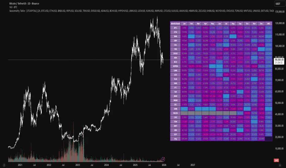
Sistema Neutro GOULART HUD Regime Radar ORB VWAPSistema Neutro GOULART is an advanced visual trading indicator that integrates:
• A unified HUD displaying session status, ORB, VWAP, risk and market bias
• A Regime Radar heatmap (GO / WAIT / NO) designed to provide clarity without chart clutter
• ORB with straight daily lines and a clean zone limited to the current session
• Direction filtering using VWAP and VWAP slope
• Condition assessment based on risk and overall market context
• A harmonized visual design focused on objective decision-making
⚠️ This indicator does NOT generate trade signals.
It provides market context, regime classification, and quality assessment to support discretionary trading decisions.
Ideal for:
• Futures markets (ES, NQ, YM)
• Day trading using ORB + VWAP
• Traders who prioritize context, discipline, and structure over signals
For educational purposes only.

Markov: Transition Matrix [Daily Timeframe]Description
This indicator computes a 3-state Markov chain from price action and visualizes the transition probabilities between daily states:
• Up: daily % change > threshold
• Down: daily % change < -threshold
• Sideways: |daily % change| ≤ threshold
From those states, it builds transition matrices:
• Today → Tomorrow (1 day ahead)
• Today → In 2 days
• Today → In 3 days
Each matrix cell shows:
P(next state | current state)
Rows are the current state (today), columns are the future state (tomorrow / +2 / +3).
Each row sums to 100% (when there is sufficient sample size).
________________________________________
How to read it (trader workflow)
1. Identify the current regime (the most recent confirmed daily state).
2. Look at the row matching that regime:
• The ★ marks the highest probability outcome for that row (most likely next state).
• Heatmap intensity increases as probability increases.
• Each row shows its own sample size (n=...) so you can judge statistical support.
3. Use Quick-read:
• “Now” = current regime
• “Best” = top conditional outcome + probability
• “2nd” = second-best outcome + probability
4. Use Universe (N):
• Shows the marginal distribution: how often days are Up/Down/Sideways across the whole dataset.
________________________________________
Settings
Core logic
• Sideways threshold: controls how strict “Sideways” is.
Example: 0.001 = ±0.10% daily move is considered Sideways.
Display
• Toggle 1D / 2D / 3D matrices.
• Highlight best probability per row (★).
• Show n per row (row transition count).
• Focus: current state row only to reduce noise and speed decision-making.
• Quick-read row for the current regime.
Theme (fully customizable)
All colors can be customized:
• Up / Down / Sideways base colors
• Header background + header text
• Values text
• Quick-read neutral background
This makes it suitable for both light and dark chart themes.
________________________________________
Notes / Limitations
• The indicator is designed for daily sessions. It uses daily close-to-close returns to classify states and update the Markov chain once per day.
• On very volatile assets, a very small threshold can make Sideways rare. If you want a more frequent Sideways regime, increase the threshold.
• This is a statistical visualization tool, not a trading system.
________________________________________
Disclaimer (TradingView-friendly)
This script is provided for educational and informational purposes only and does not constitute financial advice. Trading involves risk. Past probabilities do not guarantee future results. Use at your own discretion and always apply proper risk management.

Ichimoku MTF HeatmapGreat for flying down you watchlist, getting an idea what time frame to go to. Enjoy!

Ultimate RSI [captainua]Ultimate RSI
Overview
This indicator combines multiple RSI calculations with volume analysis, divergence detection, and trend filtering to provide a comprehensive RSI-based trading system. The script calculates RSI using three different periods (6, 14, 24) and applies various smoothing methods to reduce noise while maintaining responsiveness. The combination of these features creates a multi-layered confirmation system that reduces false signals by requiring alignment across multiple indicators and timeframes.
The script includes optimized configuration presets for instant setup: Scalping, Day Trading, Swing Trading, and Position Trading. Simply select a preset to instantly configure all settings for your trading style, or use Custom mode for full manual control. All settings include automatic input validation to prevent configuration errors and ensure optimal performance.
Configuration Presets
The script includes preset configurations optimized for different trading styles, allowing you to instantly configure the indicator for your preferred trading approach. Simply select a preset from the "Configuration Preset" dropdown menu:
- Scalping: Optimized for fast-paced trading with shorter RSI periods (4, 7, 9) and minimal smoothing. Noise reduction is automatically disabled, and momentum confirmation is disabled to allow faster signal generation. Designed for quick entries and exits in volatile markets.
- Day Trading: Balanced configuration for intraday trading with moderate RSI periods (6, 9, 14) and light smoothing. Momentum confirmation is enabled for better signal quality. Ideal for day trading strategies requiring timely but accurate signals.
- Swing Trading: Configured for medium-term positions with standard RSI periods (14, 14, 21) and moderate smoothing. Provides smoother signals suitable for swing trading timeframes. All noise reduction features remain active.
- Position Trading: Optimized for longer-term trades with extended RSI periods (24, 21, 28) and heavier smoothing. Filters are configured for highest-quality signals. Best for position traders holding trades over multiple days or weeks.
- Custom: Full manual control over all settings. All input parameters are available for complete customization. This is the default mode and maintains full backward compatibility with previous versions.
When a preset is selected, it automatically adjusts RSI periods, smoothing lengths, and filter settings to match the trading style. The preset configurations ensure optimal settings are applied instantly, eliminating the need for manual configuration. All settings can still be manually overridden if needed, providing flexibility while maintaining ease of use.
Input Validation and Error Prevention
The script includes comprehensive input validation to prevent configuration errors:
- Cross-Input Validation: Smoothing lengths are automatically validated to ensure they are always less than their corresponding RSI period length. If you set a smoothing length greater than or equal to the RSI length, the script automatically adjusts it to (RSI Length - 1). This prevents logical errors and ensures valid configurations.
- Input Range Validation: All numeric inputs have minimum and maximum value constraints enforced by TradingView's input system, preventing invalid parameter values.
- Smart Defaults: Preset configurations use validated default values that are tested and optimized for each trading style. When switching between presets, all related settings are automatically updated to maintain consistency.
Core Calculations
Multi-Period RSI:
The script calculates RSI using the standard Wilder's RSI formula: RSI = 100 - (100 / (1 + RS)), where RS = Average Gain / Average Loss over the specified period. Three separate RSI calculations run simultaneously:
- RSI(6): Uses 6-period lookback for high sensitivity to recent price changes, useful for scalping and early signal detection
- RSI(14): Standard 14-period RSI for balanced analysis, the most commonly used RSI period
- RSI(24): Longer 24-period RSI for trend confirmation, provides smoother signals with less noise
Each RSI can be smoothed using EMA, SMA, RMA (Wilder's smoothing), WMA, or Zero-Lag smoothing. Zero-Lag smoothing uses the formula: ZL-RSI = RSI + (RSI - RSI ) to reduce lag while maintaining signal quality. You can apply individual smoothing lengths to each RSI period, or use global smoothing where all three RSIs share the same smoothing length.
Dynamic Overbought/Oversold Thresholds:
Static thresholds (default 70/30) are adjusted based on market volatility using ATR. The formula: Dynamic OB = Base OB + (ATR × Volatility Multiplier × Base Percentage / 100), Dynamic OS = Base OS - (ATR × Volatility Multiplier × Base Percentage / 100). This adapts to volatile markets where traditional 70/30 levels may be too restrictive. During high volatility, the dynamic thresholds widen, and during low volatility, they narrow. The thresholds are clamped between 0-100 to remain within RSI bounds. The ATR is cached for performance optimization, updating on confirmed bars and real-time bars.
Adaptive RSI Calculation:
An adaptive RSI adjusts the standard RSI(14) based on current volatility relative to average volatility. The calculation: Adaptive Factor = (Current ATR / SMA of ATR over 20 periods) × Volatility Multiplier. If SMA of ATR is zero (edge case), the adaptive factor defaults to 0. The adaptive RSI = Base RSI × (1 + Adaptive Factor), clamped to 0-100. This makes the indicator more responsive during high volatility periods when traditional RSI may lag. The adaptive RSI is used for signal generation (buy/sell signals) but is not plotted on the chart.
Overbought/Oversold Fill Zones:
The script provides visual fill zones between the RSI line and the threshold lines when RSI is in overbought or oversold territory. The fill logic uses inclusive conditions: fills are shown when RSI is currently in the zone OR was in the zone on the previous bar. This ensures complete coverage of entry and exit boundaries. A minimum gap of 0.1 RSI points is maintained between the RSI plot and threshold line to ensure reliable polygon rendering in TradingView. The fill uses invisible plots at the threshold levels and the RSI value, with the fill color applied between them. You can select which RSI (6, 14, or 24) to use for the fill zones.
Divergence Detection
Regular Divergence:
Bullish divergence: Price makes a lower low (current low < lowest low from previous lookback period) while RSI makes a higher low (current RSI > lowest RSI from previous lookback period). Bearish divergence: Price makes a higher high (current high > highest high from previous lookback period) while RSI makes a lower high (current RSI < highest RSI from previous lookback period). The script compares current price/RSI values to the lowest/highest values from the previous lookback period using ta.lowest() and ta.highest() functions with index to reference the previous period's extreme.
Pivot-Based Divergence:
An enhanced divergence detection method that uses actual pivot points instead of simple lowest/highest comparisons. This provides more accurate divergence detection by identifying significant pivot lows/highs in both price and RSI. The pivot-based method uses a tolerance-based approach with configurable constants: 1% tolerance for price comparisons (priceTolerancePercent = 0.01) and 1.0 RSI point absolute tolerance for RSI comparisons (pivotTolerance = 1.0). Minimum divergence threshold is 1.0 RSI point (minDivergenceThreshold = 1.0). It looks for two recent pivot points and compares them: for bullish divergence, price makes a lower low (at least 1% lower) while RSI makes a higher low (at least 1.0 point higher). This method reduces false divergences by requiring actual pivot points rather than just any low/high within a period. When enabled, pivot-based divergence replaces the traditional method for more accurate signal generation.
Strong Divergence:
Regular divergence is confirmed by an engulfing candle pattern. Bullish engulfing requires: (1) Previous candle is bearish (close < open ), (2) Current candle is bullish (close > open), (3) Current close > previous open, (4) Current open < previous close. Bearish engulfing is the inverse: previous bullish, current bearish, current close < previous open, current open > previous close. Strong divergence signals are marked with visual indicators (🐂 for bullish, 🐻 for bearish) and have separate alert conditions.
Hidden Divergence:
Continuation patterns that signal trend continuation rather than reversal. Bullish hidden divergence: Price makes a higher low (current low > lowest low from previous period) but RSI makes a lower low (current RSI < lowest RSI from previous period). Bearish hidden divergence: Price makes a lower high (current high < highest high from previous period) but RSI makes a higher high (current RSI > highest RSI from previous period). These patterns indicate the trend is likely to continue in the current direction.
Volume Confirmation System
Volume threshold filtering requires current volume to exceed the volume SMA multiplied by the threshold factor. The formula: Volume Confirmed = Volume > (Volume SMA × Threshold). If the threshold is set to 0.1 or lower, volume confirmation is effectively disabled (always returns true). This allows you to use the indicator without volume filtering if desired.
Volume Climax is detected when volume exceeds: Volume SMA + (Volume StdDev × Multiplier). This indicates potential capitulation moments where extreme volume accompanies price movements. Volume Dry-Up is detected when volume falls below: Volume SMA - (Volume StdDev × Multiplier), indicating low participation periods that may produce unreliable signals. The volume SMA is cached for performance, updating on confirmed and real-time bars.
Multi-RSI Synergy
The script generates signals when multiple RSI periods align in overbought or oversold zones. This creates a confirmation system that reduces false signals. In "ALL" mode, all three RSIs (6, 14, 24) must be simultaneously above the overbought threshold OR all three must be below the oversold threshold. In "2-of-3" mode, any two of the three RSIs must align in the same direction. The script counts how many RSIs are in each zone: twoOfThreeOB = ((rsi6OB ? 1 : 0) + (rsi14OB ? 1 : 0) + (rsi24OB ? 1 : 0)) >= 2.
Synergy signals require: (1) Multi-RSI alignment (ALL or 2-of-3), (2) Volume confirmation, (3) Reset condition satisfied (enough bars since last synergy signal), (4) Additional filters passed (RSI50, Trend, ADX, Volume Dry-Up avoidance). Separate reset conditions track buy and sell signals independently. The reset condition uses ta.barssince() to count bars since the last trigger, returning true if the condition never occurred (allowing first signal) or if enough bars have passed.
Regression Forecasting
The script uses historical RSI values to forecast future RSI direction using four methods. The forecast horizon is configurable (1-50 bars ahead). Historical data is collected into an array, and regression coefficients are calculated based on the selected method.
Linear Regression: Calculates the least-squares fit line (y = mx + b) through the last N RSI values. The calculation: meanX = sumX / horizon, meanY = sumY / horizon, denominator = sumX² - horizon × meanX², m = (sumXY - horizon × meanX × meanY) / denominator, b = meanY - m × meanX. The forecast projects this line forward: forecast = b + m × i for i = 1 to horizon.
Polynomial Regression: Fits a quadratic curve (y = ax² + bx + c) to capture non-linear trends. The system of equations is solved using Cramer's rule with a 3×3 determinant. If the determinant is too small (< 0.0001), the system falls back to linear regression. Coefficients are calculated by solving: n×c + sumX×b + sumX²×a = sumY, sumX×c + sumX²×b + sumX³×a = sumXY, sumX²×c + sumX³×b + sumX⁴×a = sumX²Y. Note: Due to the O(n³) computational complexity of polynomial regression, the forecast horizon is automatically limited to a maximum of 20 bars when using polynomial regression to maintain optimal performance. If you set a horizon greater than 20 bars with polynomial regression, it will be automatically capped at 20 bars.
Exponential Smoothing: Applies exponential smoothing with adaptive alpha = 2/(horizon+1). The smoothing iterates from oldest to newest value: smoothed = alpha × series + (1 - alpha) × smoothed. Trend is calculated by comparing current smoothed value to an earlier smoothed value (at 60% of horizon): trend = (smoothed - earlierSmoothed) / (horizon - earlierIdx). Forecast: forecast = base + trend × i.
Moving Average: Uses the difference between short MA (horizon/2) and long MA (horizon) to estimate trend direction. Trend = (maShort - maLong) / (longLen - shortLen). Forecast: forecast = maShort + trend × i.
Confidence bands are calculated using RMSE (Root Mean Squared Error) of historical forecast accuracy. The error calculation compares historical values with forecast values: RMSE = sqrt(sumSquaredError / count). If insufficient data exists, it falls back to calculating standard deviation of recent RSI values. Confidence bands = forecast ± (RMSE × confidenceLevel). All forecast values and confidence bands are clamped to 0-100 to remain within RSI bounds. The regression functions include comprehensive safety checks: horizon validation (must not exceed array size), empty array handling, edge case handling for horizon=1 scenarios, division-by-zero protection, and bounds checking for all array access operations to prevent runtime errors.
Strong Top/Bottom Detection
Strong buy signals require three conditions: (1) RSI is at its lowest point within the bottom period: rsiVal <= ta.lowest(rsiVal, bottomPeriod), (2) RSI is below the oversold threshold minus a buffer: rsiVal < (oversoldThreshold - rsiTopBottomBuffer), where rsiTopBottomBuffer = 2.0 RSI points, (3) The absolute difference between current RSI and the lowest RSI exceeds the threshold value: abs(rsiVal - ta.lowest(rsiVal, bottomPeriod)) > threshold. This indicates a bounce from extreme levels with sufficient distance from the absolute low.
Strong sell signals use the inverse logic: RSI at highest point, above overbought threshold + rsiTopBottomBuffer (2.0 RSI points), and difference from highest exceeds threshold. Both signals also require: volume confirmation, reset condition satisfied (separate reset for buy vs sell), and all additional filters passed (RSI50, Trend, ADX, Volume Dry-Up avoidance).
The reset condition uses separate logic for buy and sell: resetCondBuy checks bars since isRSIAtBottom, resetCondSell checks bars since isRSIAtTop. This ensures buy signals reset based on bottom conditions and sell signals reset based on top conditions, preventing incorrect signal blocking.
Filtering System
RSI(50) Filter: Only allows buy signals when RSI(14) > 50 (bullish momentum) and sell signals when RSI(14) < 50 (bearish momentum). This filter ensures you're buying in uptrends and selling in downtrends from a momentum perspective. The filter is optional and can be disabled. Recommended to enable for noise reduction.
Trend Filter: Uses a long-term EMA (default 200) to determine trend direction. Buy signals require price above EMA, sell signals require price below EMA. The EMA slope is calculated as: emaSlope = ema - ema . Optional EMA slope filter additionally requires the EMA to be rising (slope > 0) for buy signals or falling (slope < 0) for sell signals. This provides stronger trend confirmation by requiring both price position and EMA direction.
ADX Filter: Uses the Directional Movement Index (calculated via ta.dmi()) to measure trend strength. Signals only fire when ADX exceeds the threshold (default 20), indicating a strong trend rather than choppy markets. The ADX calculation uses separate length and smoothing parameters. This filter helps avoid signals during sideways/consolidation periods.
Volume Dry-Up Avoidance: Prevents signals during periods of extremely low volume relative to average. If volume dry-up is detected and the filter is enabled, signals are blocked. This helps avoid unreliable signals that occur during low participation periods.
RSI Momentum Confirmation: Requires RSI to be accelerating in the signal direction before confirming signals. For buy signals, RSI must be consistently rising (recovering from oversold) over the lookback period. For sell signals, RSI must be consistently falling (declining from overbought) over the lookback period. The momentum check verifies that all consecutive changes are in the correct direction AND the cumulative change is significant. This filter ensures signals only fire when RSI momentum aligns with the signal direction, reducing false signals from weak momentum.
Multi-Timeframe Confirmation: Requires higher timeframe RSI to align with the signal direction. For buy signals, current RSI must be below the higher timeframe RSI by at least the confirmation threshold. For sell signals, current RSI must be above the higher timeframe RSI by at least the confirmation threshold. This ensures signals align with the larger trend context, reducing counter-trend trades. The higher timeframe RSI is fetched using request.security() from the selected timeframe.
All filters use the pattern: filterResult = not filterEnabled OR conditionMet. This means if a filter is disabled, it always passes (returns true). Filters can be combined, and all must pass for a signal to fire.
RSI Centerline and Period Crossovers
RSI(50) Centerline Crossovers: Detects when the selected RSI source crosses above or below the 50 centerline. Bullish crossover: ta.crossover(rsiSource, 50), bearish crossover: ta.crossunder(rsiSource, 50). You can select which RSI (6, 14, or 24) to use for these crossovers. These signals indicate momentum shifts from bearish to bullish (above 50) or bullish to bearish (below 50).
RSI Period Crossovers: Detects when different RSI periods cross each other. Available pairs: RSI(6) × RSI(14), RSI(14) × RSI(24), or RSI(6) × RSI(24). Bullish crossover: fast RSI crosses above slow RSI (ta.crossover(rsiFast, rsiSlow)), indicating momentum acceleration. Bearish crossover: fast RSI crosses below slow RSI (ta.crossunder(rsiFast, rsiSlow)), indicating momentum deceleration. These crossovers can signal shifts in momentum before price moves.
StochRSI Calculation
Stochastic RSI applies the Stochastic oscillator formula to RSI values instead of price. The calculation: %K = ((RSI - Lowest RSI) / (Highest RSI - Lowest RSI)) × 100, where the lookback is the StochRSI length. If the range is zero, %K defaults to 50.0. %K is then smoothed using SMA with the %K smoothing length. %D is calculated as SMA of smoothed %K with the %D smoothing length. All values are clamped to 0-100. You can select which RSI (6, 14, or 24) to use as the source for StochRSI calculation.
RSI Bollinger Bands
Bollinger Bands are applied to RSI(14) instead of price. The calculation: Basis = SMA(RSI(14), BB Period), StdDev = stdev(RSI(14), BB Period), Upper = Basis + (StdDev × Deviation Multiplier), Lower = Basis - (StdDev × Deviation Multiplier). This creates dynamic zones around RSI that adapt to RSI volatility. When RSI touches or exceeds the bands, it indicates extreme conditions relative to recent RSI behavior.
Noise Reduction System
The script includes a comprehensive noise reduction system to filter false signals and improve accuracy. When enabled, signals must pass multiple quality checks:
Signal Strength Requirement: RSI must be at least X points away from the centerline (50). For buy signals, RSI must be at least X points below 50. For sell signals, RSI must be at least X points above 50. This ensures signals only trigger when RSI is significantly in oversold/overbought territory, not just near neutral.
Extreme Zone Requirement: RSI must be deep in the OB/OS zone. For buy signals, RSI must be at least X points below the oversold threshold. For sell signals, RSI must be at least X points above the overbought threshold. This ensures signals only fire in extreme conditions where reversals are more likely.
Consecutive Bar Confirmation: The signal condition must persist for N consecutive bars before triggering. This reduces false signals from single-bar spikes or noise. The confirmation checks that the signal condition was true for all bars in the lookback period.
Zone Persistence (Optional): Requires RSI to remain in the OB/OS zone for N consecutive bars, not just touch it. This ensures RSI is truly in an extreme state rather than just briefly touching the threshold. When enabled, this provides stricter filtering for higher-quality signals.
RSI Slope Confirmation (Optional): Requires RSI to be moving in the expected signal direction. For buy signals, RSI should be rising (recovering from oversold). For sell signals, RSI should be falling (declining from overbought). This ensures momentum is aligned with the signal direction. The slope is calculated by comparing current RSI to RSI N bars ago.
All noise reduction filters can be enabled/disabled independently, allowing you to customize the balance between signal frequency and accuracy. The default settings provide a good balance, but you can adjust them based on your trading style and market conditions.
Alert System
The script includes separate alert conditions for each signal type: buy/sell (adaptive RSI crossovers), divergence (regular, strong, hidden), crossovers (RSI50 centerline, RSI period crossovers), synergy signals, and trend breaks. Each alert type has its own alertcondition() declaration with a unique title and message.
An optional cooldown system prevents alert spam by requiring a minimum number of bars between alerts of the same type. The cooldown check: canAlert = na(lastAlertBar) OR (bar_index - lastAlertBar >= cooldownBars). If the last alert bar is na (first alert), it always allows the alert. Each alert type maintains its own lastAlertBar variable, so cooldowns are independent per signal type. The default cooldown is 10 bars, which is recommended for noise reduction.
Higher Timeframe RSI
The script can display RSI from a higher timeframe using request.security(). This allows you to see the RSI context from a larger timeframe (e.g., daily RSI on an hourly chart). The higher timeframe RSI uses RSI(14) calculation from the selected timeframe. This provides context for the current timeframe's RSI position relative to the larger trend.
RSI Pivot Trendlines
The script can draw trendlines connecting pivot highs and lows on RSI(6). This feature helps visualize RSI trends and identify potential trend breaks.
Pivot Detection: Pivots are detected using a configurable period. The script can require pivots to have minimum strength (RSI points difference from surrounding bars) to filter out weak pivots. Lower minPivotStrength values detect more pivots (more trendlines), while higher values detect only stronger pivots (fewer but more significant trendlines). Pivot confirmation is optional: when enabled, the script waits N bars to confirm the pivot remains the extreme, reducing repainting. Pivot confirmation functions (f_confirmPivotLow and f_confirmPivotHigh) are always called on every bar for consistency, as recommended by TradingView. When pivot bars are not available (na), safe default values are used, and the results are then used conditionally based on confirmation settings. This ensures consistent calculations and prevents calculation inconsistencies.
Trendline Drawing: Uptrend lines connect confirmed pivot lows (green), and downtrend lines connect confirmed pivot highs (red). By default, only the most recent trendline is shown (old trendlines are deleted when new pivots are confirmed). This keeps the chart clean and uncluttered. If "Keep Historical Trendlines" is enabled, the script preserves up to N historical trendlines (configurable via "Max Trendlines to Keep", default 5). When historical trendlines are enabled, old trendlines are saved to arrays instead of being deleted, allowing you to see multiple trendlines simultaneously for better trend analysis. The arrays are automatically limited to prevent memory accumulation.
Trend Break Detection: Signals are generated when RSI breaks above or below trendlines. Uptrend breaks (RSI crosses below uptrend line) generate buy signals. Downtrend breaks (RSI crosses above downtrend line) generate sell signals. Optional trend break confirmation requires the break to persist for N bars and optionally include volume confirmation. Trendline angle filtering can exclude flat/weak trendlines from generating signals (minTrendlineAngle > 0 filters out weak/flat trendlines).
How Components Work Together
The combination of multiple RSI periods provides confirmation across different timeframes, reducing false signals. RSI(6) catches early moves, RSI(14) provides balanced signals, and RSI(24) confirms longer-term trends. When all three align (synergy), it indicates strong consensus across timeframes.
Volume confirmation ensures signals occur with sufficient market participation, filtering out low-volume false breakouts. Volume climax detection identifies potential reversal points, while volume dry-up avoidance prevents signals during unreliable low-volume periods.
Trend filters align signals with the overall market direction. The EMA filter ensures you're trading with the trend, and the EMA slope filter adds an additional layer by requiring the trend to be strengthening (rising EMA for buys, falling EMA for sells).
ADX filter ensures signals only fire during strong trends, avoiding choppy/consolidation periods. RSI(50) filter ensures momentum alignment with the trade direction.
Momentum confirmation requires RSI to be accelerating in the signal direction, ensuring signals only fire when momentum is aligned. Multi-timeframe confirmation ensures signals align with higher timeframe trends, reducing counter-trend trades.
Divergence detection identifies potential reversals before they occur, providing early warning signals. Pivot-based divergence provides more accurate detection by using actual pivot points. Hidden divergence identifies continuation patterns, useful for trend-following strategies.
The noise reduction system combines multiple filters (signal strength, extreme zone, consecutive bars, zone persistence, RSI slope) to significantly reduce false signals. These filters work together to ensure only high-quality signals are generated.
The synergy system requires alignment across all RSI periods for highest-quality signals, significantly reducing false positives. Regression forecasting provides forward-looking context, helping anticipate potential RSI direction changes.
Pivot trendlines provide visual trend analysis and can generate signals when RSI breaks trendlines, indicating potential reversals or continuations.
Reset conditions prevent signal spam by requiring a minimum number of bars between signals. Separate reset conditions for buy and sell signals ensure proper signal management.
Usage Instructions
Configuration Presets (Recommended): The script includes optimized preset configurations for instant setup. Simply select your trading style from the "Configuration Preset" dropdown:
- Scalping Preset: RSI(4, 7, 9) with minimal smoothing. Noise reduction disabled, momentum confirmation disabled for fastest signals.
- Day Trading Preset: RSI(6, 9, 14) with light smoothing. Momentum confirmation enabled for better signal quality.
- Swing Trading Preset: RSI(14, 14, 21) with moderate smoothing. Balanced configuration for medium-term trades.
- Position Trading Preset: RSI(24, 21, 28) with heavier smoothing. Optimized for longer-term positions with all filters active.
- Custom Mode: Full manual control over all settings. Default behavior matches previous script versions.
Presets automatically configure RSI periods, smoothing lengths, and filter settings. You can still manually adjust any setting after selecting a preset if needed.
Getting Started: The easiest way to get started is to select a configuration preset matching your trading style (Scalping, Day Trading, Swing Trading, or Position Trading) from the "Configuration Preset" dropdown. This instantly configures all settings for optimal performance. Alternatively, use "Custom" mode for full manual control. The default configuration (Custom mode) shows RSI(6), RSI(14), and RSI(24) with their default smoothing. Overbought/oversold fill zones are enabled by default.
Customizing RSI Periods: Adjust the RSI lengths (6, 14, 24) based on your trading timeframe. Shorter periods (6) for scalping, standard (14) for day trading, longer (24) for swing trading. You can disable any RSI period you don't need.
Smoothing Selection: Choose smoothing method based on your needs. EMA provides balanced smoothing, RMA (Wilder's) is traditional, Zero-Lag reduces lag but may increase noise. Adjust smoothing lengths individually or use global smoothing for consistency. Note: Smoothing lengths are automatically validated to ensure they are always less than the corresponding RSI period length. If you set smoothing >= RSI length, it will be auto-adjusted to prevent invalid configurations.
Dynamic OB/OS: The dynamic thresholds automatically adapt to volatility. Adjust the volatility multiplier and base percentage to fine-tune sensitivity. Higher values create wider thresholds in volatile markets.
Volume Confirmation: Set volume threshold to 1.2 (default) for standard confirmation, higher for stricter filtering, or 0.1 to disable volume filtering entirely.
Multi-RSI Synergy: Use "ALL" mode for highest-quality signals (all 3 RSIs must align), or "2-of-3" mode for more frequent signals. Adjust the reset period to control signal frequency.
Filters: Enable filters gradually to find your preferred balance. Start with volume confirmation, then add trend filter, then ADX for strongest confirmation. RSI(50) filter is useful for momentum-based strategies and is recommended for noise reduction. Momentum confirmation and multi-timeframe confirmation add additional layers of accuracy but may reduce signal frequency.
Noise Reduction: The noise reduction system is enabled by default with balanced settings. Adjust minSignalStrength (default 3.0) to control how far RSI must be from centerline. Increase requireConsecutiveBars (default 1) to require signals to persist longer. Enable requireZonePersistence and requireRsiSlope for stricter filtering (higher quality but fewer signals). Start with defaults and adjust based on your needs.
Divergence: Enable divergence detection and adjust lookback periods. Strong divergence (with engulfing confirmation) provides higher-quality signals. Hidden divergence is useful for trend-following strategies. Enable pivot-based divergence for more accurate detection using actual pivot points instead of simple lowest/highest comparisons. Pivot-based divergence uses tolerance-based matching (1% for price, 1.0 RSI point for RSI) for better accuracy.
Forecasting: Enable regression forecasting to see potential RSI direction. Linear regression is simplest, polynomial captures curves, exponential smoothing adapts to trends. Adjust horizon based on your trading timeframe. Confidence bands show forecast uncertainty - wider bands indicate less reliable forecasts.
Pivot Trendlines: Enable pivot trendlines to visualize RSI trends and identify trend breaks. Adjust pivot detection period (default 5) - higher values detect fewer but stronger pivots. Enable pivot confirmation (default ON) to reduce repainting. Set minPivotStrength (default 1.0) to filter weak pivots - lower values detect more pivots (more trendlines), higher values detect only stronger pivots (fewer trendlines). Enable "Keep Historical Trendlines" to preserve multiple trendlines instead of just the most recent one. Set "Max Trendlines to Keep" (default 5) to control how many historical trendlines are preserved. Enable trend break confirmation for more reliable break signals. Adjust minTrendlineAngle (default 0.0) to filter flat trendlines - set to 0.1-0.5 to exclude weak trendlines.
Alerts: Set up alerts for your preferred signal types. Enable cooldown to prevent alert spam. Each signal type has its own alert condition, so you can be selective about which signals trigger alerts.
Visual Elements and Signal Markers
The script uses various visual markers to indicate signals and conditions:
- "sBottom" label (green): Strong bottom signal - RSI at extreme low with strong buy conditions
- "sTop" label (red): Strong top signal - RSI at extreme high with strong sell conditions
- "SyBuy" label (lime): Multi-RSI synergy buy signal - all RSIs aligned oversold
- "SySell" label (red): Multi-RSI synergy sell signal - all RSIs aligned overbought
- 🐂 emoji (green): Strong bullish divergence detected
- 🐻 emoji (red): Strong bearish divergence detected
- 🔆 emoji: Weak divergence signals (if enabled)
- "H-Bull" label: Hidden bullish divergence
- "H-Bear" label: Hidden bearish divergence
- ⚡ marker (top of pane): Volume climax detected (extreme volume) - positioned at top for visibility
- 💧 marker (top of pane): Volume dry-up detected (very low volume) - positioned at top for visibility
- ↑ triangle (lime): Uptrend break signal - RSI breaks below uptrend line
- ↓ triangle (red): Downtrend break signal - RSI breaks above downtrend line
- Triangle up (lime): RSI(50) bullish crossover
- Triangle down (red): RSI(50) bearish crossover
- Circle markers: RSI period crossovers
All markers are positioned at the RSI value where the signal occurs, using location.absolute for precise placement.
Signal Priority and Interpretation
Signals are generated independently and can occur simultaneously. Higher-priority signals generally indicate stronger setups:
1. Multi-RSI Synergy signals (SyBuy/SySell) - Highest priority: Requires alignment across all RSI periods plus volume and filter confirmation. These are the most reliable signals.
2. Strong Top/Bottom signals (sTop/sBottom) - High priority: Indicates extreme RSI levels with strong bounce conditions. Requires volume confirmation and all filters.
3. Divergence signals - Medium-High priority: Strong divergence (with engulfing) is more reliable than regular divergence. Hidden divergence indicates continuation rather than reversal.
4. Adaptive RSI crossovers - Medium priority: Buy when adaptive RSI crosses below dynamic oversold, sell when it crosses above dynamic overbought. These use volatility-adjusted RSI for more accurate signals.
5. RSI(50) centerline crossovers - Medium priority: Momentum shift signals. Less reliable alone but useful when combined with other confirmations.
6. RSI period crossovers - Lower priority: Early momentum shift indicators. Can provide early warning but may produce false signals in choppy markets.
Best practice: Wait for multiple confirmations. For example, a synergy signal combined with divergence and volume climax provides the strongest setup.
Chart Requirements
For proper script functionality and compliance with TradingView requirements, ensure your chart displays:
- Symbol name: The trading pair or instrument name should be visible
- Timeframe: The chart timeframe should be clearly displayed
- Script name: "Ultimate RSI " should be visible in the indicator title
These elements help traders understand what they're viewing and ensure proper script identification. The script automatically includes this information in the indicator title and chart labels.
Performance Considerations
The script is optimized for performance:
- ATR and Volume SMA are cached using var variables, updating only on confirmed and real-time bars to reduce redundant calculations
- Forecast line arrays are dynamically managed: lines are reused when possible, and unused lines are deleted to prevent memory accumulation
- Calculations use efficient Pine Script functions (ta.rsi, ta.ema, etc.) which are optimized by TradingView
- Array operations are minimized where possible, with direct calculations preferred
- Polynomial regression automatically caps the forecast horizon at 20 bars (POLYNOMIAL_MAX_HORIZON constant) to prevent performance degradation, as polynomial regression has O(n³) complexity. This safeguard ensures optimal performance even with large horizon settings
- Pivot detection includes edge case handling to ensure reliable calculations even on early bars with limited historical data. Regression forecasting functions include comprehensive safety checks: horizon validation (must not exceed array size), empty array handling, edge case handling for horizon=1 scenarios, and division-by-zero protection in all mathematical operations
The script should perform well on all timeframes. On very long historical data, forecast lines may accumulate if the horizon is large; consider reducing the forecast horizon if you experience performance issues. The polynomial regression performance safeguard automatically prevents performance issues for that specific regression type.
Known Limitations and Considerations
- Forecast lines are forward-looking projections and should not be used as definitive predictions. They provide context but are not guaranteed to be accurate.
- Dynamic OB/OS thresholds can exceed 100 or go below 0 in extreme volatility scenarios, but are clamped to 0-100 range. This means in very volatile markets, the dynamic thresholds may not widen as much as the raw calculation suggests.
- Volume confirmation requires sufficient historical volume data. On new instruments or very short timeframes, volume calculations may be less reliable.
- Higher timeframe RSI uses request.security() which may have slight delays on some data feeds.
- Regression forecasting requires at least N bars of history (where N = forecast horizon) before it can generate forecasts. Early bars will not show forecast lines.
- StochRSI calculation requires the selected RSI source to have sufficient history. Very short RSI periods on new charts may produce less reliable StochRSI values initially.
Practical Use Cases
The indicator can be configured for different trading styles and timeframes:
Swing Trading: Select the "Swing Trading" preset for instant optimal configuration. This preset uses RSI periods (14, 14, 21) with moderate smoothing. Alternatively, manually configure: Use RSI(24) with Multi-RSI Synergy in "ALL" mode, combined with trend filter (EMA 200) and ADX filter. This configuration provides high-probability setups with strong confirmation across multiple RSI periods.
Day Trading: Select the "Day Trading" preset for instant optimal configuration. This preset uses RSI periods (6, 9, 14) with light smoothing and momentum confirmation enabled. Alternatively, manually configure: Use RSI(6) with Zero-Lag smoothing for fast signal detection. Enable volume confirmation with threshold 1.2-1.5 for reliable entries. Combine with RSI(50) filter to ensure momentum alignment. Strong top/bottom signals work well for day trading reversals.
Trend Following: Enable trend filter (EMA) and EMA slope filter for strong trend confirmation. Use RSI(14) or RSI(24) with ADX filter to avoid choppy markets. Hidden divergence signals are useful for trend continuation entries.
Reversal Trading: Focus on divergence detection (regular and strong) combined with strong top/bottom signals. Enable volume climax detection to identify capitulation moments. Use RSI(6) for early reversal signals, confirmed by RSI(14) and RSI(24).
Forecasting and Planning: Enable regression forecasting with polynomial or exponential smoothing methods. Use forecast horizon of 10-20 bars for swing trading, 5-10 bars for day trading. Confidence bands help assess forecast reliability.
Multi-Timeframe Analysis: Enable higher timeframe RSI to see context from larger timeframes. For example, use daily RSI on hourly charts to understand the larger trend context. This helps avoid counter-trend trades.
Scalping: Select the "Scalping" preset for instant optimal configuration. This preset uses RSI periods (4, 7, 9) with minimal smoothing, disables noise reduction, and disables momentum confirmation for faster signals. Alternatively, manually configure: Use RSI(6) with minimal smoothing (or Zero-Lag) for ultra-fast signals. Disable most filters except volume confirmation. Use RSI period crossovers (RSI(6) × RSI(14)) for early momentum shifts. Set volume threshold to 1.0-1.2 for less restrictive filtering.
Position Trading: Select the "Position Trading" preset for instant optimal configuration. This preset uses extended RSI periods (24, 21, 28) with heavier smoothing, optimized for longer-term trades. Alternatively, manually configure: Use RSI(24) with all filters enabled (Trend, ADX, RSI(50), Volume Dry-Up avoidance). Multi-RSI Synergy in "ALL" mode provides highest-quality signals.
Practical Tips and Best Practices
Getting Started: The fastest way to get started is to select a configuration preset that matches your trading style. Simply choose "Scalping", "Day Trading", "Swing Trading", or "Position Trading" from the "Configuration Preset" dropdown to instantly configure all settings optimally. For advanced users, use "Custom" mode for full manual control. The default configuration (Custom mode) is balanced and works well across different markets. After observing behavior, customize settings to match your trading style.
Reducing Repainting: All signals are based on confirmed bars, minimizing repainting. The script uses confirmed bar data for all calculations to ensure backtesting accuracy.
Signal Quality: Multi-RSI Synergy signals in "ALL" mode provide the highest-quality signals because they require alignment across all three RSI periods. These signals have lower frequency but higher reliability. For more frequent signals, use "2-of-3" mode. The noise reduction system further improves signal quality by requiring multiple confirmations (signal strength, extreme zone, consecutive bars, optional zone persistence and RSI slope). Adjust noise reduction settings to balance signal frequency vs. accuracy.
Filter Combinations: Start with volume confirmation, then add trend filter for trend alignment, then ADX filter for trend strength. Combining all three filters significantly reduces false signals but also reduces signal frequency. Find your balance based on your risk tolerance.
Volume Filtering: Set volume threshold to 0.1 or lower to effectively disable volume filtering if you trade instruments with unreliable volume data or want to test without volume confirmation. Standard confirmation uses 1.2-1.5 threshold.
RSI Period Selection: RSI(6) is most sensitive and best for scalping or early signal detection. RSI(14) provides balanced signals suitable for day trading. RSI(24) is smoother and better for swing trading and trend confirmation. You can disable any RSI period you don't need to reduce visual clutter.
Smoothing Methods: EMA provides balanced smoothing with moderate lag. RMA (Wilder's smoothing) is traditional and works well for RSI. Zero-Lag reduces lag but may increase noise. WMA gives more weight to recent values. Choose based on your preference for responsiveness vs. smoothness.
Forecasting: Linear regression is simplest and works well for trending markets. Polynomial regression captures curves and works better in ranging markets. Exponential smoothing adapts to trends. Moving average method is most conservative. Use confidence bands to assess forecast reliability.
Divergence: Strong divergence (with engulfing confirmation) is more reliable than regular divergence. Hidden divergence indicates continuation rather than reversal, useful for trend-following strategies. Pivot-based divergence provides more accurate detection by using actual pivot points instead of simple lowest/highest comparisons. Adjust lookback periods based on your timeframe: shorter for day trading, longer for swing trading. Pivot divergence period (default 5) controls the sensitivity of pivot detection.
Dynamic Thresholds: Dynamic OB/OS thresholds automatically adapt to volatility. In volatile markets, thresholds widen; in calm markets, they narrow. Adjust the volatility multiplier and base percentage to fine-tune sensitivity. Higher values create wider thresholds in volatile markets.
Alert Management: Enable alert cooldown (default 10 bars, recommended) to prevent alert spam. Each alert type has its own cooldown, so you can set different cooldowns for different signal types. For example, use shorter cooldown for synergy signals (high quality) and longer cooldown for crossovers (more frequent). The cooldown system works independently for each signal type, preventing spam while allowing different signal types to fire when appropriate.
Technical Specifications
- Pine Script Version: v6
- Indicator Type: Non-overlay (displays in separate panel below price chart)
- Repainting Behavior: Minimal - all signals are based on confirmed bars, ensuring accurate backtesting results
- Performance: Optimized with caching for ATR and volume calculations. Forecast arrays are dynamically managed to prevent memory accumulation.
- Compatibility: Works on all timeframes (1 minute to 1 month) and all instruments (stocks, forex, crypto, futures, etc.)
- Edge Case Handling: All calculations include safety checks for division by zero, NA values, and boundary conditions. Reset conditions and alert cooldowns handle edge cases where conditions never occurred or values are NA.
- Reset Logic: Separate reset conditions for buy signals (based on bottom conditions) and sell signals (based on top conditions) ensure logical correctness.
- Input Parameters: 60+ customizable parameters organized into logical groups for easy configuration. Configuration presets available for instant setup (Scalping, Day Trading, Swing Trading, Position Trading, Custom).
- Noise Reduction: Comprehensive noise reduction system with multiple filters (signal strength, extreme zone, consecutive bars, zone persistence, RSI slope) to reduce false signals.
- Pivot-Based Divergence: Enhanced divergence detection using actual pivot points for improved accuracy.
- Momentum Confirmation: RSI momentum filter ensures signals only fire when RSI is accelerating in the signal direction.
- Multi-Timeframe Confirmation: Optional higher timeframe RSI alignment for trend confirmation.
- Enhanced Pivot Trendlines: Trendline drawing with strength requirements, confirmation, and trend break detection.
Technical Notes
- All RSI values are clamped to 0-100 range to ensure valid oscillator values
- ATR and Volume SMA are cached for performance, updating on confirmed and real-time bars
- Reset conditions handle edge cases: if a condition never occurred, reset returns true (allows first signal)
- Alert cooldown handles na values: if no previous alert, cooldown allows the alert
- Forecast arrays are dynamically sized based on horizon, with unused lines cleaned up
- Fill logic uses a minimum gap (0.1) to ensure reliable polygon rendering in TradingView
- All calculations include safety checks for division by zero and boundary conditions. Regression functions validate that horizon doesn't exceed array size, and all array access operations include bounds checking to prevent out-of-bounds errors
- The script uses separate reset conditions for buy signals (based on bottom conditions) and sell signals (based on top conditions) for logical correctness
- Background coloring uses a fallback system: dynamic color takes priority, then RSI(6) heatmap, then monotone if both are disabled
- Noise reduction filters are applied after accuracy filters, providing multiple layers of signal quality control
- Pivot trendlines use strength requirements to filter weak pivots, reducing noise in trendline drawing. Historical trendlines are stored in arrays and automatically limited to prevent memory accumulation when "Keep Historical Trendlines" is enabled
- Volume climax and dry-up markers are positioned at the top of the pane for better visibility
- All calculations are optimized with conditional execution - features only calculate when enabled (performance optimization)
- Input Validation: Automatic cross-input validation ensures smoothing lengths are always less than RSI period lengths, preventing configuration errors
- Configuration Presets: Four optimized preset configurations (Scalping, Day Trading, Swing Trading, Position Trading) for instant setup, plus Custom mode for full manual control
- Constants Management: Magic numbers extracted to documented constants for improved maintainability and easier tuning (pivot tolerance, divergence thresholds, fill gap, etc.)
- TradingView Function Consistency: All TradingView functions (ta.crossover, ta.crossunder, ta.atr, ta.lowest, ta.highest, ta.lowestbars, ta.highestbars, etc.) and custom functions that depend on historical results (f_consecutiveBarConfirmation, f_rsiSlopeConfirmation, f_rsiZonePersistence, f_applyAllFilters, f_rsiMomentum, f_forecast, f_confirmPivotLow, f_confirmPivotHigh) are called on every bar for consistency, as recommended by TradingView. Results are then used conditionally when needed. This ensures consistent calculations and prevents calculation inconsistencies.

Simulateur Carnet d'Ordres & Liquidité [Sese] - Custom🔹 Indicator Name
Order Book & Liquidity Simulator - Custom
🔹 Concept and Functionality
This indicator is a technical analysis tool designed to visually simulate market depth (Order Book) and potential liquidity zones.
It is important to adhere to TradingView's transparency rules: This script does not access real Level 2 data (the actual exchange order book). Instead, it uses a deductive algorithm based on historical Price Action to estimate where Buy Limit (Bid) and Sell Limit (Ask) orders might be resting.
Methodology used by the script:
Pivot Detection: The indicator scans for significant Swing Highs and Swing Lows over a user-defined lookback period (Length).
Level Projection: These pivots are projected to the right as horizontal lines.
Red Lines (Ask): Represent potential resistance zones (sellers).
Blue Lines (Bid): Represent potential support zones (buyers).
Liquidity Management (Absorption): The script is dynamic. If the current price crosses a line, the indicator assumes the liquidity at that level has been consumed (orders filled). The line is then automatically deleted from the chart.
Density Profile (Right Side): Horizontal bars appear to the right of the current price. These approximate a "Time Price Opportunity" or Volume Profile, showing where the market has spent the most time recently.
🔹 User Manual (Settings)
Here is how to configure the inputs to match your trading style:
1. Detection Algorithm
Lookback Length (Candles): Determines the sensitivity of the pivots.
Low value (e.g., 10): Shows many lines (scalping/short term).
High value (e.g., 50): Shows only major structural levels (swing trading).
Volume Factor: (Technical note: In this specific code version, this variable is calculated but the lines are primarily drawn based on geometric pivots).
2. Visual Settings
Show Price Lines (Bid/Ask): Toggles the horizontal Support/Resistance lines on or off.
Show Volume Profile: Toggles the heatmap-style bars on the right side of the chart.
Extend Lines: If checked, untouched lines will extend to the right towards the current price bar.
3. Colors and Transparency Management
Customize the aesthetics to keep your chart clean:
Bid / Ask Colors: Choose your base colors (Default is Blue and Red).
Line Transparency (%): Crucial for chart visibility.
0% = Solid, bright colors.
80-90% = Very subtle, faint lines (recommended if you overlay this on other tools).
Text Size: Adjusts the size of the price labels ("BUY LIMIT" / "SELL LIMIT").
🔹 How to Read the Indicator
Rejections: Unbroken lines act as potential walls. Watch for price reaction when approaching a blue line (support) or red line (resistance).
Breakouts/Absorption: When a line disappears, it means the level has been breached. The market may then seek the next liquidity level (the next line).
Density (Right-side boxes): More opaque/visible boxes indicate a price zone "accepted" by the market (consolidation). Empty gaps suggest an imbalance where price might move through quickly.
⚠️ Disclaimer
This script is for educational and technical analysis purposes only. It is a simulation based on price history, not real-time order book data. Past performance is not indicative of future results. Trading involves risk.

Low Volatility Profiles [BigBeluga]🔵 OVERVIEW
Low Volatility Profiles is a market compression and breakout-anticipation tool that identifies phases of low volatility using ADX and then builds a real-time volume profile inside the detected range.
This helps traders spot accumulation/distribution zones and prepare for explosive moves when volatility expands.
When volatility is low ➜ price coils ➜ volume organizes ➜ breakouts become highly actionable.
This tool visualizes that process with dynamic range boxes + volume bins + PoC extension.
🔵 CONCEPTS
Low-Volatility Detection — Uses ADX threshold & cross logic to define volatility contraction regimes.
Range Construction — Draws a price box that expands with highs/lows during the compression phase.
Micro Volume Profile — Builds a volume histogram inside the range using bins (micro volume nodes).
Delta Calculation — Tracks positive vs negative volume to gauge buyer/seller pressure within range.
Point of Control (PoC) — Highlights the price level with max traded volume inside the range.
PoC Extension — Optionally extends PoC into future bars to show potential reaction zone after breakout.
Breakout Validation — Ends the profile zone when price breaks above or below the modeled range.
Noise Removal — Automatically removes invalid or small ranges to prevent chart clutter.
This tool turns consolidation into actionable structure by exposing where smart money accumulates before trending moves.
🔵 FEATURES
ADX-Driven Range Detection — Identify when market transitions into low-volatility compression.
Configurable ADX Threshold — Set sensitivity for contraction zones.
Cross-Type Option — Detect low volatility via cross under / crossover logic.
Dynamic Range Box — Expands live with price as contraction unfolds.
Micro Volume Profile (Bins) — Distributes volume across bins inside range for micro POC mapping.
Volume Delta Visualization — Shows imbalance inside consolidation (accumulation vs distribution).
Real-Time PoC Highlight — Instantly shows most traded price inside the compression.
PoC Extension Mode — Extend PoC forward to project reaction levels post-breakout.
Clean Auto-Reset Logic — Removes boxes if range invalid or breakout occurs too fast.
Optional Filled Boxes — Heatmap-style profile visualization inside range body.
ADX Line + Threshold Plot — Visual assistance for volatility state monitoring.
🔵 HOW TO USE
Identify Accumulation Zones — When price enters low-volatility ADX condition and profile builds.
Watch the PoC — PoC acts as battle zone; move above/below can signal initiator strength.
Breakout Strategy — Trade break above/below the range after compression.
Mean Reversion Inside Range — Fade edges while price remains inside compression box.
Combine With Trend Tools — Use trend confirmation (MA/EMA/Flow indicators) after breakout.
Use Delta Clues — Positive delta tilt suggests accumulation; negative suggests distribution.
Monitor Range Size — Longer build + high PoC volume = stronger potential breakout energy.
🔵 CONCLUSION
Low Volatility Profiles isolates accumulation phases and maps volume concentration before volatility expansion.
By combining ADX compression, micro volume distribution, and PoC tracing, traders gain an edge in anticipating powerful breakout cycles and institutional positioning.
Trade the quiet moment before the storm — where smart money prepares the move, and the real opportunity emerges.

Monitor Posición Bollinger Multi-TFThis indicator provides a comprehensive dashboard that allows you to monitor the price position relative to Bollinger Bands across 7 different timeframes simultaneously, without the need to switch charts.
It uses the %B (Percent B) logic to normalize the price position, giving you an instant "Heatmap" view of the market state (Overbought/Oversold) from the 1-minute chart up to the Weekly chart.
Key Features:
Multi-Timeframe Monitoring: Watch 1m, 5m, 15m, 1h, 4h, Daily, and Weekly timeframes in a single panel.
Dynamic Color Coding:
Dark Red: Price breaking above the Upper Band (>100%).
Light Red: Price near the Upper Band (Resistance zone).
Gray: Price in the neutral middle zone.
Light Green: Price near the Lower Band (Support zone).
Dark Green: Price breaking below the Lower Band (<0%).
Trend Arrows: Indicates momentum (▲ or ▼) based on the previous candle's position.
Current Timeframe Highlight: Automatically highlights the row corresponding to your current chart view in orange.
Fully Customizable: Adjust Bollinger settings (Length, Mult), choose your preferred timeframes, and change the table position/size.
Movable Panel: Includes X/Y offset settings to prevent the table from blocking price action or menu buttons.
How to Use:
Add the indicator to your chart.
Use the dashboard to spot confluence across timeframes.
Example: If 15m, 1H, and 4H are all showing Red, the asset is likely overextended to the upside.
Example: If the lower timeframes are turning Green while the higher timeframes remain Gray/Bullish, it might indicate a pullback opportunity.
Settings:
Bollinger Config: Length (20) and Multiplier (2.0) by default.
Timeframes: Select the 7 specific TFs you want to track.
Visuals: Change table position, text size, and offset coordinates.
This tool is essential for scalpers and day traders who need situational awareness across multiple fractals instantly.

Filter Ribbon1. Indicator Name
Filter Ribbon
2. One-line Introduction
A trend visualization ribbon that uses linear regression and directional scoring to highlight bullish and bearish strength with intuitive color gradients.
3. General Overview
Filter Ribbon is a minimalistic yet powerful trend visualization tool that leverages linear regression slope ordering to determine directional momentum. It analyzes the ordering of regression values over a defined lookback period and quantifies how consistently the price has been trending upward or downward.
Using a pairwise comparison system, it calculates a trend "score" and compares this to a configurable threshold to determine if a bullish, bearish, or neutral condition exists.
The result is a color-coded ribbon that sits over the chart, changing hue and opacity based on both the direction and strength of the trend. The stronger the directional alignment, the more opaque the ribbon becomes, offering traders a fast, intuitive way to assess market sentiment at a glance.
It also includes an optional linear regression line to further help visualize the central trend.
This indicator is best used in trend-following systems or as a dynamic background layer when combined with signal-based strategies.
Thanks to its efficient design and protected logic, Filter Ribbon offers high-performance visualization without compromising strategy integrity.
4. Key Advantages
🌈 Visual Trend Heatmap
Dynamic color ribbon gives real-time visual feedback on both trend direction and strength.
🔢 Quantified Trend Scoring
Calculates a mathematically sound trend score using pairwise linear regression comparisons.
⚖️ Adjustable Sensitivity
Users can tune lookback and threshold parameters to fit different asset classes and timeframes.
📉 Smooth Ribbon Effect
Plots upper/lower bands around regression line with smooth filling for a professional chart look.
🎯 Precise Trend Confirmation
Acts as a confidence layer for other entry/exit signals by confirming broader trend bias.
🔒 Secure and Minimal Codebase
Core logic is embedded securely with minimal exposure, reducing risk of replication or misuse.
📘 Indicator User Guide
📌 Basic Concept
Filter Ribbon determines trend direction and intensity by comparing the order of linear regression values over time.
It forms a ribbon on the chart that changes color based on trend direction and opacity based on trend strength.
This makes it ideal for identifying clear trending periods vs. uncertain consolidations.
⚙️ Settings Explained
Lookback Period: Number of bars for scoring the trend direction (higher = smoother trend)
Range Tolerance (%): Determines how aggressive the trend classification is (lower = stricter)
Regression Length: Period for calculating the base linear regression line
Ribbon Colors: Customize colors for bullish and bearish conditions
📈 Bullish Timing Example
Ribbon color is green and becomes increasingly opaque
Regression line slopes upward and price remains above it
Can be used as trend confirmation for long trades
📉 Bearish Timing Example
Ribbon color is red with higher opacity
Price consistently below the regression line
Useful for confirming short trade setups or avoiding long entries
🧪 Recommended Use Cases
Combine with breakout indicators to validate if the breakout aligns with broader trend
Use in swing or trend-following strategies as a background filter
Helps filter out trades during unclear, sideways market conditions
🔒 Precautions
Not a signal generator on its own — meant for trend context only
Ribbon may lag slightly during sudden trend reversals; best used with reactive entry tools
Always test ribbon parameters on your specific market/timeframe before applying live
Avoid using solely in low-volatility or flat markets — sensitivity may require tuning
+++

Rotation SentinelROTATION SENTINEL v1.1 — OVERVIEW
Rotation Sentinel is a macro rotation engine that tracks 10 institutional-grade dominance, liquidity, and trend signals to identify when capital is flowing into altcoins.
Each row outputs Green / Yellow / Red, and the system produces a 0–10 Rotation Score plus a final regime:
🔴 NO ROTATION (0–4)
🟡 ROTATION STARTING (5–6)
🟢 ALTSEASON (7–10)
Use on Daily timeframe for best accuracy.
KEY SIGNALS
1️⃣ BTC.D ex-stables
Shows true BTC vs alt strength.
🟢 Falling = capital rotating into alts.
🔴 Rising = alts bleeding. (Master switch.)
2️⃣ OTHERS.D
Broad altcoin dominance.
🟢 Rising = early alt strength.
🔴 Falling = weak participation.
3️⃣ ETH/BTC
Rotation ignition.
🟢 ETH outperforming = rotation can start.
🔴 ETH lagging = altseason impossible.
4️⃣ STABLE.C.D
Crypto “fear index.”
🟢 Falling = risk-on environment.
🔴 Rising = capital hiding in stables.
5️⃣ USDT.D
Real-time risk positioning.
🟢 Falling = capital deploying.
🔴 Rising = defensive.
6️⃣ TOTAL3 (HTF Trend)
Structural alt market health.
🟢 Above SMA + rising = bullish structure.
🔴 Below SMA + falling = systematic weakness.
7️⃣ TOTAL3 / TOTAL2
Depth of rotation.
🟢 Mid/small caps outperforming = deep rotation.
🔴 Only large caps moving = shallow cycle.
8️⃣ Risk Ratio (OTHERS.D / STABLE.C.D)
Pure risk appetite.
🟢 Alts gaining on stables = risk-on.
9️⃣ OTHERS/BTC
Alt value vs BTC.
🟢 Rising = alts outperforming BTC.
🔟 Liquidation Heatmap (Manual)
Update from Hyblock/Coinalyze.
🟢 Liquidity above = upside easier.
ALTSEASON TRIGGER
Fires only when all 6 core conditions turn GREEN:
BTC.D ex-stables
OTHERS.D
ETH/BTC
STABLE.C.D
TOTAL3 structure
Rotation Score ≥ threshold (default 7)
BEST PRACTICES
Use Daily timeframe (macro rotation, not intraday noise)
Score < 5 → defensive / selective trades
Score 5–6 → early rotation window
Score ≥ 7 → confirmed altseason regime
Let alerts notify you; no need to manually monitor
INCLUDED ALERTS
🚨 ALTSEASON TRIGGERED
⚠️ Rotation Score Crossed Threshold
📈 ETH/BTC Rotation Clock Activated
🔥 OTHERS.D Breaking Higher

BTC Macro Heatmap (Fed Cuts & Hikes)🔴 1. Red line – Fed Funds Rate (policy trend)
This line tells you what stage of the monetary cycle we’re in.
Rising red line = the Fed is hiking → liquidity is tightening → money leaves risk assets like BTC.
Flat = pause → markets start pricing in the next move (often sideways BTC).
Falling = easing / cutting → liquidity returns → bullish environment builds.
The rate of change matters more than the level. When the slope turns down, capital starts seeking yield again — BTC benefits first because it’s the most volatile asset.
💚 2. Dim green zones – detected cuts
These are data-based easing events pulled directly from FRED.
They show when the actual effective rate began moving down, not necessarily the exact meeting day.
Think of them as the Fed’s “foot off the brake” — that’s when risk markets begin responding.
🟩 3. Bright green lines – official FOMC cuts
These are the real policy shifts — the Fed formally changed direction.
After these appear, BTC historically transitions from accumulation → markup phase.
Look at 2020: the bright green lines came right before BTC’s full reversal.
You’re seeing the same thing now with the 2025 lines — early-stage liquidity return.
🟠 4. Orange line – DXY (US Dollar Index)
DXY is your “risk-off” gauge.
When DXY rises, global investors flock to dollars → BTC usually weakens.
When DXY peaks and starts dropping, it means risk appetite is coming back → BTC rallies.
BTC and DXY are inversely correlated about 70–80% of the time.
Watch for DXY lower highs after rate cuts — that’s your macro confirmation of a BTC-friendly environment.
🟦 5. Aqua line – BTC (normalized)
You’re not looking for the price itself here, but its shape relative to DXY and the Fed line.
When BTC curls up as the red line flattens and DXY rolls over → that’s historically the start of a major bull phase.
BTC tends to bottom before the first cut and explode once DXY decisively breaks down.
🧠 Putting it together
Here’s the rhythm this chart shows over and over:
Fed hikes (red line rising) → BTC weakens, DXY climbs.
Fed pauses (red line flat) → BTC stops falling, DXY tops.
Fed cuts (dim + bright green) → DXY turns down → BTC begins long recovery → bull cycle starts.
