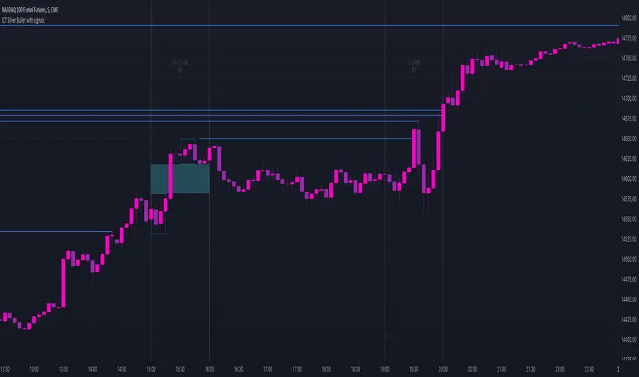
ICT Silver Bullet with signals
The "ICT Silver Bullet with signals" indicator (inspired from the lectures of "The Inner Circle Trader" (ICT)),
goes a step further than the ICT Silver Bullet publication, which I made for LuxAlgo :
• uses HTF candles
• instant drawing of Support & Resistance (S/R) lines when price retraces into FVG
• NWOG - NDOG S/R lines
• signals
The Silver Bullet (SB) window which is a specific 1-hour interval where a Fair Value Gap (FVG) pattern can be formed.
When price goes back to the FVG, without breaking it, Support & Resistance lines will be drawn immediately.
There are 3 different Silver Bullet windows (New York local time):
The London Open Silver Bullet (03 AM — 04 AM ~ 03:00 — 04:00)
The AM Session Silver Bullet (10 AM — 11 AM ~ 10:00 — 11:00)
The PM Session Silver Bullet (02 PM — 03 PM ~ 14:00 — 15:00)
🔶 USAGE
This technique can visualise potential support/resistance lines, which can be used as targets.
The script contains 2 main components:
• forming of a Fair Value Gap (FVG)
• drawing support/resistance (S/R) lines
🔹 Forming of FVG
When HTF candles forms an FVG, the FVG will be drawn at the end (close) of the last HTF candle.
To make it easier to visualise the 2 HTF candles that form the FVG, you can enable
• SHOW -> HTF candles
During the SB session, when a FVG is broken, the FVG will be removed, together with its S/R lines.
The same goes if price did not retrace into FVG at the last bar of the SB session
Only exception is when "Remove broken FVG's" is disabled.
In this case a FVG can be broken, as long as price bounces back before the end of the SB session, it will remain to be visible:
🔹 Drawing support/resistance lines
S/R target lines are drawn immediately when price retraces into the FVG.
They will remain updated until they are broken (target hit)
Potential S/R lines are formed by:
• previous swings (swing settings (left-right)
• New Week Opening Gap (NWOG): close on Friday - weekly open
• New Day Opening Gap (NWOG): close previous day - current daily open
Only non-broken lines are included.
Broken =
• minimum of open and close below potential S/R line
• maximum of open and close above potential S/R line
NDOG lines are coloured fuchsia (as in the ICT lectures), NWOG are coloured white (darkmode) or black (lightmode ~ ICT lectures)
Swing line colour can be set as desired.
Here S/R includes NDOG lines:
The same situation, with "Extend Target-lines to their source" enabled:
Here with NWOG lines:
This publication contains a "Minimum Trade Framework (mTFW)", which represents the best-case expected price delivery, this is not your actual trade entry - exit range.
• 40 ticks for index futures or indices
• 15 pips for Forex pairs
The minimum distance (if applicable) can be shown by enabling "Show" - "Minimum Trade Framework" -> blue arrow from close to mTFW
Potential S/R lines needs to be higher (bullish) or lower (bearish) than mTFW.
🔶 SETTINGS
(check USAGE for deeper insights and explanation)
🔹 Only last x bars: when enabled, the script will do most of the calculations at these last x candles, potentially this can speeds calculations.
🔹 Swing settings (left-right): Sets the length, which will set the lookback period/sensitivity of the ZigZag patterns (which directs the trend and points for S/R lines)
🔹 FVG
HTF (minutes): 1-15 minutes.
• When the chart TF is equal of higher, calculations are based on current TF.
• Chart TF > 15 minutes will give the warning: "Please use a timeframe <= 15 minutes".
Remove broken FVG's: when enabled the script will remove FVG (+ associated S/R lines) immediately when FVG is broken at opposite direction.
FVG's still will be automatically removed at the end of the SB session, when there is no retrace, together with associated S/R lines,...
~ trend: Only include FVG in the same direction as the current trend
Note -> when set 'right' (swing setting) rather high ( > 3), he trend change will be delayed as well (default 'right' max 5)
Extend: extend FVG to max right side of SB session
🔹 Targets – support/resistance
Extend Target-lines to their source: extend lines to their origin
Colours (Swing S/R lines)
🔹 Show
SB session: show lines and labels of SB session (+ colour)
• Labels can be disabled separately in the 'Style' section, colour is set at the 'Inputs' section
Trend : Show trend (ZigZag, coloured ~ trend)
HTF candles: Show the 2 HTF candles that form the FVG
Minimum Trade Framework: blue arrow (if applicable)
🔶 ALERTS
There are 4 signals provided (bullish/bearish):
FVG Formed
FVG Retrace
Target reached
FVG cancelled
You can choose between dynamic alerts - only 1 alert needs to be set for all signals, or you can set specific alerts as desired.
💜 PURPLE BARS 😈
• Since TradingView has chosen to give away our precious Purple coloured Wizard Badge, bars are coloured purple 😊😉
Поиск скриптов по запросу "机械革命无界15+时不时闪屏"
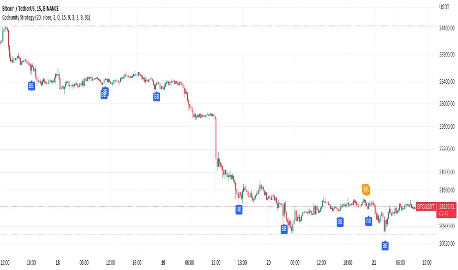
Code Unity 1.0Bitcoin 15 minutes strategy.
Bitcoin 15 minutes strategy.
Bitcoin 15 minutes strategy.
Bitcoin 15 minutes strategy.
Bitcoin 15 minutes strategy.
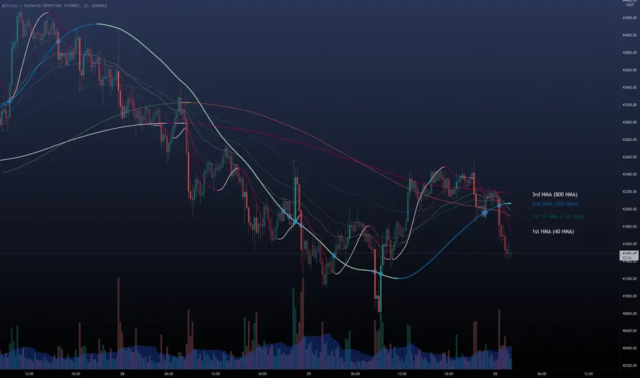
Multi HMA Lines by NB(ENG)
The Hull Moving Average (HMA) line responds quickly to volatile markets,
sometimes it provides more accurate information than the Exponancital Moving Average (EMA).
In particular, the 200 HMA line is easy to decide the overall trend of the market,
and it serves the basis entry position.
So I made indicator that provides these HMA lines into various periods so that they can be checked in one.
In addition, a custom TimeFrame HMA line function has been added so that you can check
not only the TimeFrame that meets your trading standards, but also the HMA of the other TimeFrame that you custome sets.
For example, if you want to see the 200 HMA of the 60-minute bar, you can select and set the different TimeFrame in the Multi TF section below.
For reference, 200 HMA at the 15-minute bar is the same value as 50 HMA at the 1-hour bar, so as shown in the following chart,
I use 4 HMA lines at the 15-minute bar : 20 HMA, 50 HMA, 200 HMA, and 200 HMA from 60-minute TimeFrame.
We hope it will help you in your trading. :)
(KOR)
HMA(Hull Moving Average) 라인은 변동성이 심한 시장에 빠르게 반응하며,
때때로 EMA(Exponancital Moving Average)보다 더 정확한 정보를 제공하곤 합니다.
특히 200HMA 라인은 시장의 전반적인 추세를 판단하기에 용이하며,
큰 틀에서의 포지션 진입 근거의 기반이 됩니다.
이러한 HMA 라인을 다양한 기간으로 나누어 하나의 지표에서 확인 할 수 있도록 만들어 보았습니다.
아울러, 자신의 매매 기준에 맞는 타임 프레임은 물론, 다른 타임 프레임의 HMA도 확인 할 수 있도록
커스텀 타임 프레임 HMA 라인 기능을 추가로 넣었습니다.
예를 들어, 15분 타임 프레임이 본인 매매 기준표이지만, 60분 봉의 200 HMA도 보고 싶다면
밑의 Multi TF 항목에서 해당 타임 프레임을 선택 후 설정하시면 됩니다.
참고로 15분 봉에서의 200 HMA은 1시간 봉에서의 50 HMA과 동일한 값이므로 저는 다음 차트 그림과 같이
15분 봉에서 20 HMA, 50 HMA, 200 HMA, 그리고 1시간 봉에서 200 HMA 이렇게 4개의 라인을 참고 하고 있습니다.
여러분 거래에 도움이 되기를 바랍니다. :)
Cowabunga System from babypips.comPlease do read the information below as well, especially if you are new to Forex.
The Cowabunga System is a type of Mechanical Trading System that filters trades based on the trend of the 4 hour chart with EMAs and some other familiar indicators (RSI, Stochastics and MACD) while entering trades base on 15 minute chart.
I have coded (quite amateurishly) the basic system onto a 15 minute chart (the 4 hour settings are coded as well). The author says the system is to be traded off the 15 minute chart with the 4 hour chart only as a reference for trend direction.
4 Hour Chart Settings
5 EMA
10 EMA
Stochastics (10,3,3)
RSI (9)
Then we move onto the 15 minute chart, where he gives us the trade entry rules.
15 Minute Chart Settings
5 EMA
10 EMA
Stochastics (10,3,3)
RSI (9)
MACD (12,26,9)
Entry Rules - long entry rules used, obviously reverse these for shorting.
1. EMA must cross above the 10 EMA.
2. RSI must be greater than 50 and not overbought.
3. Stochastic must be headed up and not be in overbought territory.
4. MACD histogram must go from negative to positive OR be negative and start to increase in value.
What I did.
1. Set the RSI and Stochastic levels to avoid entries when they indicate overbought conditions for long and oversold conditions for short (80 and 20 levels).
2. Users can input specific times they want to backtest.
3. User's can configure profit targets, trailing stops and stops. Default is set it to was 100 pips profit target with a 40 pip trailing stop. (Note, when you are changing these values, please note that each pip is worth 10, so 100 pips is entered as 1000.)
The Cowabunga System from babypips.com is another popular and active system. The author, Pip Surfer, continues to post wins and losses with this system. It shows there is a lot of honesty and integrity with this system if the author keeps up to date even 10 years later and is not afraid of sharing the times the system causes losses.
As an example of this, here is post he shared just last week . It's almost like a journal, he gives specific times and reasons why he entered, lets the readers know when he was stopped out, etc. I think that what he does is equally important as his system.
To read more about this system, visit the thread on babypips.com, click here.

Stochastic BTC OptimizedEnhanced Stochastic for Bitcoin (BTC) – Optimized for Daily Timeframe
This enhanced Stochastic oscillator is specifically fine-tuned for BTC/USD on the 1D timeframe, leveraging historical data from Bitstamp (2011–2025) to minimize false signals and maximize reliability in Bitcoin's volatile swings.
Unlike the classic Stochastic (14, 3, 3), this version uses optimized parameters:
- K Period = 21 – smoother reaction, better suited for BTC’s macro cycles
- D Period = 3, Smooth K = 3 – reduces noise while preserving responsiveness
- Overbought = 85, Oversold = 15 – accounts for BTC’s tendency to trend strongly within extreme zones without immediate reversal
✅ Smart Signal Logic:
Buy/sell signals appear only when %K crosses %D inside the oversold (≤15) or overbought (≥85) zones, and only the first signal is shown to avoid whipsaws.
Visual Enhancements:
- Thick lines when %K/%D are in overbought/oversold zones
- Green/red background highlights on valid signals
- Optional up/down arrows for clear entry visualization
- Customizable colors, line widths, and transparency
🔒 No alerts included – clean, focused on price action and momentum.
💡 Pro Tip: For even higher accuracy, use this indicator in combination with a long-term trend filter (e.g., EMA 200). The oscillator excels in ranging or retracement phases but should not be used alone in strong parabolic moves.
Based on Mozilla Public License v2.0 – feel free to use, modify, and share. Perfect for swing traders and long-term Bitcoin analysts seeking high-probability reversal zones.
перевод на русский
Улучшенный Stochastic для Bitcoin (BTC) — оптимизирован для дневного таймфрейма
Этот улучшенный осциллятор Stochastic специально настроен под BTC/USD на дневном графике, с учётом исторических данных Bitstamp (2011–2025), чтобы минимизировать ложные сигналы и повысить надёжность в условиях высокой волатильности биткоина.
В отличие от классического Stochastic (14, 3, 3), эта версия использует оптимизированные параметры:
- Период K = 21 — более плавная реакция, лучше соответствует макроциклам BTC
- Период D = 3, Сглаживание K = 3 — снижает шум, сохраняя отзывчивость
- Уровень перекупленности = 85, перепроданности = 15 — учитывает склонность BTC к сильным трендам в экстремальных зонах без немедленного разворота
✅ Интеллектуальная логика сигналов:
Покупка/продажа отображается только при пересечении %K и %D внутри зоны перепроданности (≤15) или перекупленности (≥85), и только первый сигнал фиксируется, чтобы избежать «хлыстов».
Улучшенная визуализация:
- Жирные линии, когда %K/%D находятся в экстремальных зонах
- Зелёный/красный фон при появлении сигналов
- Опциональные стрелки для чёткого отображения точек входа
- Настройка цветов, толщины линий и прозрачности
🔒 Без алертов — чистый инструмент, сфокусированный на цене и импульсе.
💡 Совет профессионала: для ещё большей точности используйте этот индикатор вместе с трендовым фильтром (например, EMA 200). Осциллятор лучше всего работает в фазах консолидации или отката, но не стоит применять его в одиночку во время сильных параболических движений.
На основе Mozilla Public License v2.0 — свободно используйте, модифицируйте и делитесь. Идеален для свинг-трейдеров и аналитиков Bitcoin, ищущих зоны с высокой вероятностью разворота.

Altseason IndexDescription of the "Altseason Index" Indicator
The Altseason Index is a powerful and visually minimalist tool designed to objectively identify the onset and conclusion of an "altseason" in the cryptocurrency market. Moving beyond subjective speculation, this indicator employs a clear, mathematical methodology by comparing the performance of a broad basket of altcoins against Bitcoin.
🎯 Core Concept and Utility
An "Altseason" is a market period where altcoins (cryptocurrencies other than Bitcoin) consistently yield higher returns than BTC. This indicator empowers traders and investors to:
Objectively Identify Market Cycles: Precisely pinpoint when capital is actively rotating from Bitcoin into altcoins and vice versa.
Make Data-Driven Decisions: Adjust their strategy in a timely manner: increasing exposure to altcoins during an altseason or rotating back into BTC upon its conclusion.
Avoid Emotional Pitfalls: Steer clear of FOMO (Fear Of Missing Out) and base decisions on hard data rather than market noise.
⚙️ How the Calculation Works
1. Asset Selection: The indicator tracks the performance of 15 leading altcoins across various market segments (Layer 1s, DeFi, Meme, Payments), ensuring a representative sample.
2. Performance Comparison: For each altcoin, the percentage price change over the user-defined lookback period (default: 90 days) is calculated. This performance is then compared to BTC's performance over the same period.
3. Counting the "Outperformers": The index counts the number of altcoins that have "outperformed" BTC.
4. Calculating the Index: The Altseason Index value is the percentage of altcoins in the basket that are outperforming BTC. For example, a value of 60% means that 9 out of the 15 coins performed better than Bitcoin.
🛠️ Indicator Settings
The settings are kept simple and intuitive, allowing you to customize the indicator to your strategy:
Lookback Period (days) (Default: 90):
- Defines the time horizon for the performance calculation.
- Shorter Periods (30-60 days) react faster to new trends but may produce more false signals.
- Longer Periods (90-180 days) provide smoother and more reliable signals, capturing sustained macro-trends.
Altseason Threshold (%) (Default: 75%):
- This is the key parameter that defines what index value constitutes an official "altseason."
- A threshold of 75% means an altseason is declared when at least 11 out of the 15 altcoins (75%) are outperforming BTC.
- You can increase the threshold (e.g., to 85%) for more conservative and stronger signals, or decrease it (e.g., to 65%) for earlier entries.
📊 Interpreting the Readings and Signals
The indicator uses a clear color-coding system and levels for easy interpretation:
🔴 < 30%: "BTC SEASON"
Bitcoin is dominating. The market is in risk-off mode or a state of anticipation. Growth is concentrated in BTC.
⚪ 30% - 49%: "NEUTRAL"
A transitional phase. The market is uncertain. Some alts show strength, but there is no unified trend.
🔵 50% - 74%: "BULLISH"
Growing strength in altcoins. Capital is beginning to rotate actively. This can be an early stage of an altseason.
🟢 ≥ 75% (or your custom threshold): "ALTSEASON"
The active altseason phase. The vast majority of altcoins are rising faster than BTC. This is the period of maximum potential returns for alts.
Signal Markers:
Green Dot: Signals the potential start of an altseason (the index crosses above the threshold).
Red Dot: Signals the potential end of an altseason (the index crosses below the threshold).
ℹ️ Information Panel
The chart displays two clean information panels:
1. Main Info Label:
Current index value (e.g., ⟠ 80%).
Market status (ALTSEASON, BULLISH, etc.).
The ratio of outperforming altcoins (11/15 alts).
2. Dominance & Market Cap Panel:
Alts: Altcoin Dominance (the market cap share of all coins except BTC).
BTC: Bitcoin Dominance.
Market: Total cryptocurrency market capitalization in billions of USD. This helps assess the overall market context (bullish/bearish).
💎 Conclusion
The Altseason Index is your strategic companion for navigating the crypto markets. It transforms the complex task of identifying market cycles into a simple and visual process. Use it to confirm broad market trends, identify potential entry and exit points, and, most importantly, to maintain discipline in your trading strategy by filtering out noise and emotion.
Disclaimer: This indicator is a tool for analysis and does not constitute investment advice. All trading decisions are taken at your own risk.

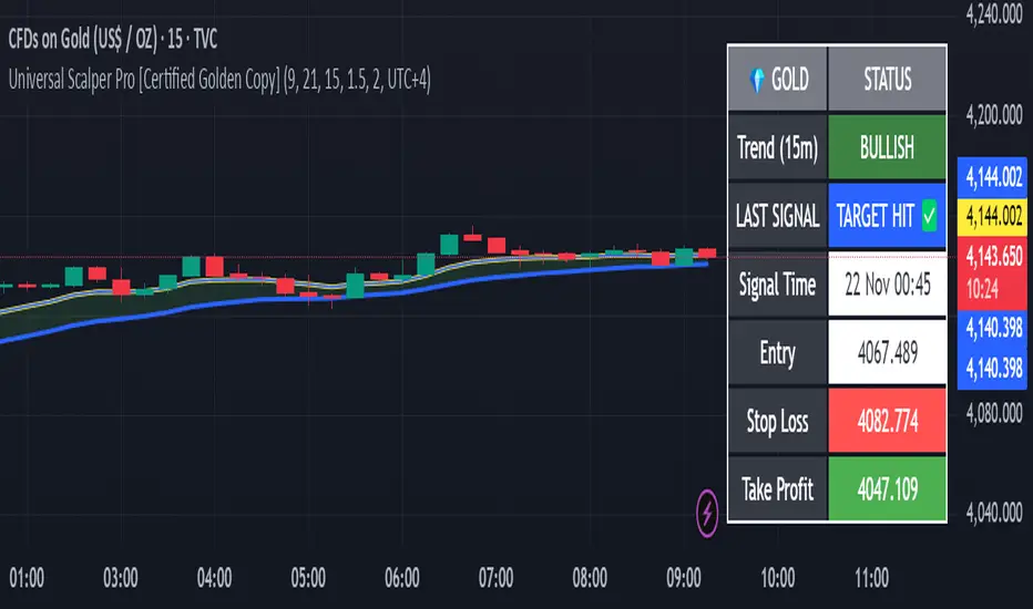
Universal Scalper Indicator [Crypto/Forex/Gold]Universal Scalper Pro is an all-in-one scalping system designed for the 15-Minute Timeframe. It automates the analysis of trend, volatility, and risk management into a single, high-contrast dashboard.
Unlike standard crossover indicators, this system filters out low-volatility "noise" using a built-in ADX engine and automatically calculates dynamic Stop Loss and Take Profit levels based on market volatility (ATR).
It is engineered to work universally on:
Crypto (BTC, ETH, SOL, Altcoins)
Commodities (Gold, Silver, Oil)
Forex (Major & Minor Pairs)
Stocks (High volume tech stocks like NVDA, TSLA)
📈 How It Works (The Strategy)
1. The Trend Engine (9/21 EMA) The core logic utilizes a Fast (9) and Slow (21) Exponential Moving Average crossover.
Bullish Signal: The 9 EMA crosses above the 21 EMA.
Bearish Signal: The 9 EMA crosses below the 21 EMA. This specific combination is chosen for its responsiveness to 15-minute intraday trends.
2. The Noise Filter (ADX > 15) To prevent "whipsaws" (fake signals during sideways markets), the script includes a Volatility Filter based on the Average Directional Index (ADX).
Signals are rejected if the ADX is below 15.
This ensures you only receive alerts when there is sufficient momentum to sustain a move.
3. Dynamic Risk Management (ATR) The script uses the Average True Range (ATR) to calculate Stop Loss and Take Profit levels that adapt to the specific asset's volatility.
Stop Loss: Placed at 1.5x ATR from the entry. (Tight enough to preserve capital, wide enough to survive standard market noise).
Take Profit: Placed at 2.0x ATR from the entry. (Provides a healthy 1:1.3 Risk/Reward ratio).
🚀 Key Features
Universal Dashboard: A bottom-right panel displays the live Trend Status, Entry Price, Stop Loss, and Take Profit. It automatically formats decimals for any asset (e.g., 2 decimals for Gold, 5 for Forex, 8 for Crypto).
"Sticky" Memory: The dashboard retains the prices of the last valid signal, allowing you to manage your trade even after the signal candle closes.
Trend Cloud: A visual Green/Red zone between the EMAs helps you instantly identify the market bias.
Unified Alerts: A single alert setup ("Any alert() function call") sends the Asset Name, Entry, SL, and TP directly to your phone.
🛠️ How to Use
Timeframe: Set your chart to 15 Minutes (15m).
Wait for the Signal: Look for the "BUY" (Green) or "SELL" (Red) label on the chart.
Check the Dashboard: Ensure the "STATUS" is BULLISH (for buys) or BEARISH (for sells). If the status says "WAIT", do not trade.
Execute: Enter the trade using the exact Stop Loss and Take Profit levels shown on the dashboard.
⚠️ Risk Disclaimer
Trading financial markets involves high risk and may not be suitable for all investors. This indicator is a technical analysis tool and does not constitute financial advice. Past performance is not indicative of future results. Always practice with a demo account before trading real capital.
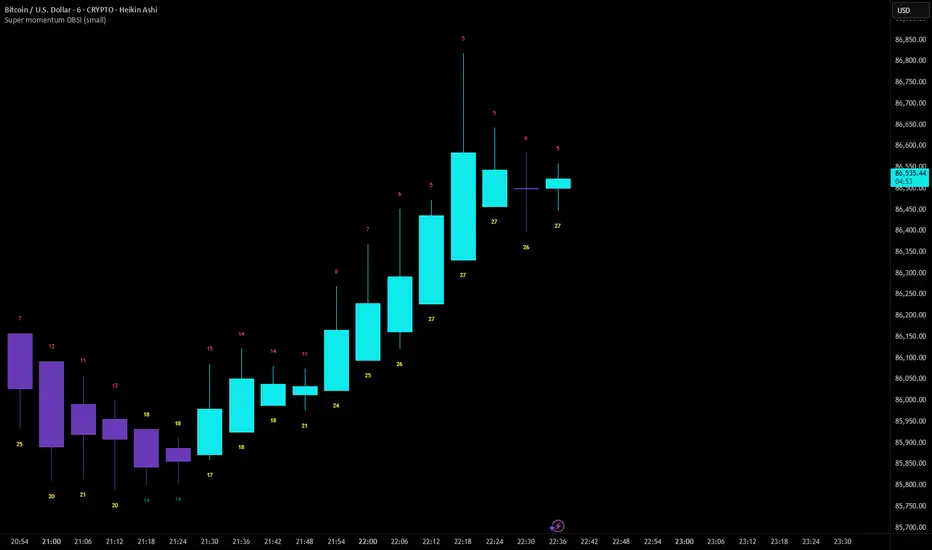
Super momentum DBSISuper momentum DBSI: The Ultimate Guide
1. What is this Indicator?
The Super momentum DBSI is a "Consensus Engine." Instead of relying on a single line (like an RSI) to tell you where the market is going, this tool calculates 33 distinct technical indicators simultaneously for every single candle.
It treats the market like a democracy. It asks 33 mathematical "voters" (Momentum, Trend, Volume, Volatility) if they are Bullish or Bearish.
If 30 out of 33 say "Buy," the score is high (Yellow), and the trend is extremely strong.
If only 15 say "Buy," the score is low (Teal), and the trend is weak or choppy.
2. Visual Guide: How to Read the Numbers
The Scores
Top Number (Bears): Represents Selling Pressure.
Bottom Number (Bulls): Represents Buying Pressure.
The Colors (The Traffic Lights)
The colors are your primary signal. They tell you who is currently winning the war.
🟡 YELLOW (Dominance):
This indicates the Winning Side.
If the Bottom Number is Yellow, Bulls are in control.
If the Top Number is Yellow, Bears are in control.
🔴 RED (Weakness):
This appears on the Top. It means Bears are present but losing.
🔵 TEAL (Weakness):
This appears on the Bottom. It means Bulls are present but losing.
3. Trading Strategy
Scenario A: The "Strong Buy" (Long Entry)
The Setup: You are looking for a shift in momentum where Buyers overwhelm Sellers.
Watch the Bottom Number: Wait for it to turn Yellow.
Confirm Strength: Ensure the score is above 15 and rising (e.g., 12 → 18 → 22).
Check the Top: The Top Number should be Red and low (below 10).
Trigger: Enter on the candle close.
Scenario B: The "Strong Sell" (Short Entry)
The Setup: You are looking for Sellers to crush the Buyers.
Watch the Top Number: Wait for it to turn Yellow.
Confirm Strength: Ensure the score is above 15 and rising.
Check the Bottom: The Bottom Number should be Teal and low.
Trigger: Enter on the candle close.
Scenario C: The "No Trade Zone" (Choppy Market)
The Setup: The market is confused.
Visual: Top is Red, Bottom is Teal.
Meaning: NOBODY IS WINNING. There is no Yellow number.
Action: Do not trade. This usually happens during lunch hours, weekends, or right before big news. This filter alone will save you from many false breakouts.
4. What is Inside? (The 33 Indicators)
To give you confidence in the signals, here is exactly what the script is checking:
Group 1: Momentum (Oscillators)
Detects if price is moving fast.
RSI (Relative Strength Index)
CCI (Commodity Channel Index)
Stochastic
Williams %R
Momentum
Rate of Change (ROC)
Ultimate Oscillator
Awesome Oscillator
True Strength Index (TSI)
Stoch RSI
TRIX
Chande Momentum Oscillator
Group 2: Trend Direction
Detects the general path of the market.
13. MACD
14. Parabolic SAR
15. SuperTrend
16. ALMA (Moving Average)
17. Aroon
18. ADX (Directional Movement)
19. Coppock Curve
20. Ichimoku Conversion Line
21. Hull Moving Average
Group 3: Price Action
Detects where price is relative to averages.
22. Price vs EMA 20
23. Price vs EMA 50
24. Price vs EMA 200
Group 4: Volume & Force
Detects if there is money behind the move.
25. Money Flow Index (MFI)
26. On Balance Volume (OBV)
27. Chaikin Money Flow (CMF)
28. VWAP (Intraday)
29. Elder Force Index
30. Ease of Movement
Group 5: Volatility
Detects if price is pushing the outer limits.
31. Bollinger Bands
32. Keltner Channels
33. Donchian Channels
5. Pro Tips for Success
Don't Catch Knives: If the Bear score (Top) is Yellow and 25+, do not try to buy the dip. Wait for the Yellow score to break.
Exit Early: If you are Long and the Yellow Bull score drops from 28 to 15 in one candle, TAKE PROFIT. The momentum has died.
Use Higher Timeframes: This indicator works best on 15m, 1H, and 4H charts. On the 1m chart, it may be too volatile.
Pre-Market ORB Break and Retest - Institutional═══════════════════════════════════
PRE-MARKET ORB BREAK AND RETEST - INSTITUTIONAL
═══════════════════════════════════
Free professional Pre-Market Opening Range Breakout indicator from QuantCrawler - your AI-powered futures trading analysis platform.
Built as a free resource for the trading community. Support us at quantcrawler.com and on YouTube @AutomateWithAaron.
═══════════════════════════════════
📊 HOW IT WORKS
1. Captures the 8:00-8:15 AM ET pre-market range where institutional investors position
2. Draws OR High, OR Low, and Midpoint levels on your chart
3. Waits for market open at 9:30 AM EST before detecting breakouts
4. Fires LONG/SHORT entry signals when price retests the OR midpoint after breakout
═══════════════════════════════════
✓ FEATURES
- Runs on 1m or 5m charts - captures 15m pre-market range automatically
- Zone marked at 8:15 AM, trades trigger after 9:30 AM market open
- Universal - works on futures, forex, stocks, and crypto
- Customizable sessions - NY, London, Asia, or any custom timeframe
- Adjustable breakout distance to match your instrument
- Clean visual signals - only shows actionable entries
- Session end time stops monitoring after market close
═══════════════════════════════════
⚙️ SETTINGS
- Breakout Distance (Points): Distance outside OR zone to confirm breakout
- Timezone: Select your trading session
- Opening Range Time: Pre-market positioning window (default 8:00-8:15)
- Session End Time: When to stop monitoring (default 16:00)
═══════════════════════════════════
🎯 IDEAL FOR
Day traders who defend institutional positioning levels. The 8:00-8:15 AM range captures where smart money positions before retail market open, giving you an edge on key support/resistance zones.
═══════════════════════════════════
🚀 WANT MORE?
This indicator pairs perfectly with QuantCrawler's AI-powered chart analysis:
- Multi-timeframe futures analysis (15m/5m/1m scalping, 4H/1H/30m intraday, 1D/4H/1H swing)
- Precision entry points, stop losses, and profit targets
- Confidence scoring for every setup
- Covers futures, forex, and crypto markets
Visit quantcrawler.com to see how AI can level up your trading.
═══════════════════════════════════
⚠️ DISCLAIMER
This indicator is for educational purposes only. Past performance does not guarantee future results. Always use proper risk management and never risk more than you can afford to lose.
═══════════════════════════════════
Built with ❤️ by Aaron at QuantCrawler
quantcrawler.com | AI-Powered Futures Trading Analysis

15m ORB BREAK AND RETEST - MIDPOINT═══════════════════════════════════
15m ORB BREAK AND RETEST - MIDPOINT
═══════════════════════════════════
Free professional 15-minute Opening Range Breakout indicator from QuantCrawler - your AI-powered futures trading analysis platform.
Built as a free resource for the trading community. Support us at quantcrawler.com and on YouTube @AutomateWithAaron.
═══════════════════════════════════
📊 HOW IT WORKS
1. Captures the 15-minute Opening Range (default: 9:30-9:45 AM ET)
2. Draws OR High, OR Low, and Midpoint levels on your chart
3. Detects breakouts when price closes beyond the OR zone + your specified distance
4. Fires LONG/SHORT entry signals when price retests the OR midpoint after breakout
═══════════════════════════════════
✓ FEATURES
- Runs on 1m or 5m charts - captures 15m opening range automatically
- Universal - works on futures, forex, stocks, and crypto
- Customizable sessions - NY, London, Asia, or any custom timeframe
- Adjustable breakout distance to match your instrument
- Clean visual signals - only shows actionable entries
- Session end time stops monitoring after market close
═══════════════════════════════════
⚙️ SETTINGS
- Breakout Distance (Points): Distance outside OR zone to confirm breakout
- Timezone: Select your trading session
- Opening Range Time: First 15 minutes to capture (default 9:30-9:45)
- Session End Time: When to stop monitoring (default 16:00)
═══════════════════════════════════
🎯 IDEAL FOR
Day traders and swing traders who prefer wider opening ranges for reduced noise. The 15-minute OR provides more stable support/resistance levels compared to 5m setups.
═══════════════════════════════════
🚀 WANT MORE?
This indicator pairs perfectly with QuantCrawler's AI-powered chart analysis:
- Multi-timeframe futures analysis (15m/5m/1m scalping, 4H/1H/30m intraday, 1D/4H/1H swing)
- Precision entry points, stop losses, and profit targets
- Confidence scoring for every setup
- Covers futures, forex, and crypto markets
Visit quantcrawler.com to see how AI can level up your trading.
═══════════════════════════════════
⚠️ DISCLAIMER
This indicator is for educational purposes only. Past performance does not guarantee future results. Always use proper risk management and never risk more than you can afford to lose.
═══════════════════════════════════
Built with ❤️ by Aaron and QuantCrawler
quantcrawler.com | AI-Powered Futures Trading Analysis

Pair Cointegration & Static Beta Analyzer (v6)Pair Cointegration & Static Beta Analyzer (v6)
This indicator evaluates whether two instruments exhibit statistical properties consistent with cointegration and tradable mean reversion.
It uses long-term beta estimation, spread standardization, AR(1) dynamics, drift stability, tail distribution analysis, and a multi-factor scoring model.
1. Static Beta and Spread Construction
A long-horizon static beta is estimated using covariance and variance of log-returns.
This beta does not update on every bar and is used throughout the entire model.
Beta = Cov(r1, r2) / Var(r2)
Spread = PriceA - Beta * PriceB
This “frozen” beta provides structural stability and avoids rolling noise in spread construction.
2. Correlation Check
Log-price correlation ensures the instruments move together over time.
Correlation ≥ 0.85 is required before deeper cointegration diagnostics are considered meaningful.
3. Z-Score Normalization and Distribution Behavior
The spread is standardized:
Z = (Spread - MA(Spread)) / Std(Spread)
The following statistical properties are examined:
Z-Mean: Should be close to zero in a stationary process
Z-Variance: Measures amplitude of deviations
Tail Probability: Frequency of |Z| being larger than a threshold (e.g. 2)
These metrics reveal whether the spread behaves like a mean-reverting equilibrium.
4. Mean Drift Stability
A rolling mean of the spread is examined.
If the rolling mean drifts excessively, the spread may not represent a stable long-term equilibrium.
A normalized drift ratio is used:
Mean Drift Ratio = Range( RollingMean(Spread) ) / Std(Spread)
Low drift indicates stable long-run equilibrium behavior.
5. AR(1) Dynamics and Half-Life
An AR(1) model approximates mean reversion:
Spread(t) = Phi * Spread(t-1) + error
Mean reversion requires:
0 < Phi < 1
Half-life of reversion:
Half-life = -ln(2) / ln(Phi)
Valid half-life for 10-minute bars typically falls between 3 and 80 bars.
6. Composite Scoring Model (0–100)
A multi-factor weighted scoring system is applied:
Component Score
Correlation 0–20
Z-Mean 0–15
Z-Variance 0–10
Tail Probability 0–10
Mean Drift 0–15
AR(1) Phi 0–15
Half-Life 0–15
Score interpretation:
70–100: Strong Cointegration Quality
40–70: Moderate
0–40: Weak
A pair is classified as cointegrated when:
Total Score ≥ Threshold (default = 70)
7. Main Cointegration Panel
Displays:
Static beta
Log-price correlation
Z-Mean, Z-Variance, Tail Probability
Drift Ratio
AR(1) Phi and Half-life
Composite score
Overall cointegration assessment
8. Beta Hedge Position Sizing (Average-Price Based)
To provide a more stable hedge ratio, hedge sizing is computed using average prices, not instantaneous prices:
AvgPriceA = SMA(PriceA, N)
AvgPriceB = SMA(PriceB, N)
Required B per 1 A = Beta * (AvgPriceA / AvgPriceB)
Using averaged prices results in a smoother, more reliable hedge ratio, reducing noise from bar-to-bar volatility.
The panel displays:
Required B security for 1 A security (average)
This represents the beta-neutral quantity of B required to hedge one unit of A.
Overview of Classical Stationarity & Cointegration Methods
The principal econometric tools commonly used in assessing stationarity and cointegration include:
Augmented Dickey–Fuller (ADF) Test
Phillips–Perron (PP) Test
KPSS Test
Engle–Granger Cointegration Test
Phillips–Ouliaris Cointegration Test
Johansen Cointegration Test
Since these procedures rely on regression residuals, matrix operations, and distribution-based critical values that are not supported in TradingView Pine Script, a practical multi-criteria scoring approach is employed instead. This framework leverages metrics that are fully computable in Pine and offers an operational proxy for evaluating cointegration-like behavior under platform constraints.
References
Engle & Granger (1987), Co-integration and Error Correction
Poterba & Summers (1988), Mean Reversion in Stock Prices
Vidyamurthy (2004), Pairs Trading
Explanation structured with assistance from OpenAI’s ChatGPT
Regards.

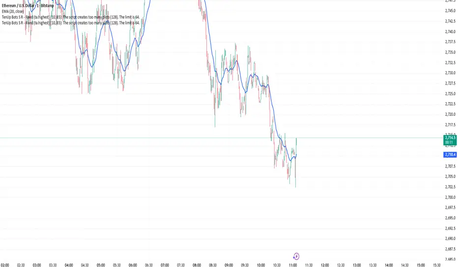
TenUp Bots S R - Fixed (ta.highest)//@version=5
indicator("TenUp Bots S R - Fixed (ta.highest)", overlay = true)
// Inputs
a = input.int(10, "Sensitivity (bars)", minval = 1, maxval = 9999)
d_pct = input.int(85, "Transparency (%)", minval = 0, maxval = 100)
// Convert 0-100% to 0-255 transparency (color.new uses 0..255)
transp = math.round(d_pct * 255 / 100)
// Colors with transparency applied
resColor = color.new(color.red, transp)
supColor = color.new(color.blue, transp)
// Helper (calculations only)
getRes(len) => ta.highest(high, len)
getSup(len) => ta.lowest(low, len)
// === PLOTS (all in global scope) ===
plot(getRes(a*1), title="Resistance 1", color=resColor, linewidth=2)
plot(getSup(a*1), title="Support 1", color=supColor, linewidth=2)
plot(getRes(a*2), title="Resistance 2", color=resColor, linewidth=2)
plot(getSup(a*2), title="Support 2", color=supColor, linewidth=2)
plot(getRes(a*3), title="Resistance 3", color=resColor, linewidth=2)
plot(getSup(a*3), title="Support 3", color=supColor, linewidth=2)
plot(getRes(a*4), title="Resistance 4", color=resColor, linewidth=2)
plot(getSup(a*4), title="Support 4", color=supColor, linewidth=2)
plot(getRes(a*5), title="Resistance 5", color=resColor, linewidth=2)
plot(getSup(a*5), title="Support 5", color=supColor, linewidth=2)
plot(getRes(a*6), title="Resistance 6", color=resColor, linewidth=2)
plot(getSup(a*6), title="Support 6", color=supColor, linewidth=2)
plot(getRes(a*7), title="Resistance 7", color=resColor, linewidth=2)
plot(getSup(a*7), title="Support 7", color=supColor, linewidth=2)
plot(getRes(a*8), title="Resistance 8", color=resColor, linewidth=2)
plot(getSup(a*8), title="Support 8", color=supColor, linewidth=2)
plot(getRes(a*9), title="Resistance 9", color=resColor, linewidth=2)
plot(getSup(a*9), title="Support 9", color=supColor, linewidth=2)
plot(getRes(a*10), title="Resistance 10", color=resColor, linewidth=2)
plot(getSup(a*10), title="Support 10", color=supColor, linewidth=2)
plot(getRes(a*15), title="Resistance 15", color=resColor, linewidth=2)
plot(getSup(a*15), title="Support 15", color=supColor, linewidth=2)
plot(getRes(a*20), title="Resistance 20", color=resColor, linewidth=2)
plot(getSup(a*20), title="Support 20", color=supColor, linewidth=2)
plot(getRes(a*25), title="Resistance 25", color=resColor, linewidth=2)
plot(getSup(a*25), title="Support 25", color=supColor, linewidth=2)
plot(getRes(a*30), title="Resistance 30", color=resColor, linewidth=2)
plot(getSup(a*30), title="Support 30", color=supColor, linewidth=2)
plot(getRes(a*35), title="Resistance 35", color=resColor, linewidth=2)
plot(getSup(a*35), title="Support 35", color=supColor, linewidth=2)
plot(getRes(a*40), title="Resistance 40", color=resColor, linewidth=2)
plot(getSup(a*40), title="Support 40", color=supColor, linewidth=2)
plot(getRes(a*45), title="Resistance 45", color=resColor, linewidth=2)
plot(getSup(a*45), title="Support 45", color=supColor, linewidth=2)
plot(getRes(a*50), title="Resistance 50", color=resColor, linewidth=2)
plot(getSup(a*50), title="Support 50", color=supColor, linewidth=2)
plot(getRes(a*75), title="Resistance 75", color=resColor, linewidth=2)
plot(getSup(a*75), title="Support 75", color=supColor, linewidth=2)
plot(getRes(a*100), title="Resistance 100", color=resColor, linewidth=2)
plot(getSup(a*100), title="Support 100", color=supColor, linewidth=2)
plot(getRes(a*150), title="Resistance 150", color=resColor, linewidth=2)
plot(getSup(a*150), title="Support 150", color=supColor, linewidth=2)
plot(getRes(a*200), title="Resistance 200", color=resColor, linewidth=2)
plot(getSup(a*200), title="Support 200", color=supColor, linewidth=2)
plot(getRes(a*250), title="Resistance 250", color=resColor, linewidth=2)
plot(getSup(a*250), title="Support 250", color=supColor, linewidth=2)
plot(getRes(a*300), title="Resistance 300", color=resColor, linewidth=2)
plot(getSup(a*300), title="Support 300", color=supColor, linewidth=2)
plot(getRes(a*350), title="Resistance 350", color=resColor, linewidth=2)
plot(getSup(a*350), title="Support 350", color=supColor, linewidth=2)
plot(getRes(a*400), title="Resistance 400", color=resColor, linewidth=2)
plot(getSup(a*400), title="Support 400", color=supColor, linewidth=2)
plot(getRes(a*450), title="Resistance 450", color=resColor, linewidth=2)
plot(getSup(a*450), title="Support 450", color=supColor, linewidth=2)
plot(getRes(a*500), title="Resistance 500", color=resColor, linewidth=2)
plot(getSup(a*500), title="Support 500", color=supColor, linewidth=2)
plot(getRes(a*750), title="Resistance 750", color=resColor, linewidth=2)
plot(getSup(a*750), title="Support 750", color=supColor, linewidth=2)
plot(getRes(a*1000), title="Resistance 1000", color=resColor, linewidth=2)
plot(getSup(a*1000), title="Support 1000", color=supColor, linewidth=2)
plot(getRes(a*1250), title="Resistance 1250", color=resColor, linewidth=2)
plot(getSup(a*1250), title="Support 1250", color=supColor, linewidth=2)
plot(getRes(a*1500), title="Resistance 1500", color=resColor, linewidth=2)
plot(getSup(a*1500), title="Support 1500", color=supColor, linewidth=2)
Golden Cross 50/200 EMATrend-following systems are characterized by having a low win rate, yet in the right circumstances (trending markets and higher timeframes) they can deliver returns that even surpass those of systems with a high win rate.
Below, I show you a simple bullish trend-following system with clear execution rules:
System Rules
-Long entries when the 50-period EMA crosses above the 200-period EMA.
-Stop Loss (SL) placed at the lowest low of the 15 candles prior to the entry candle.
-Take Profit (TP) triggered when the 50-period EMA crosses below the 200-period EMA.
Risk Management
-Initial capital: $10,000
-Position size: 10% of capital per trade
-Commissions: 0.1% per trade
Important Note:
In the code, the stop loss is defined using the swing low (15 candles), but the position size is not adjusted based on the distance to the stop loss. In other words, 10% of the equity is risked on each trade, but the actual loss on the trade is not controlled by a maximum fixed percentage of the account — it depends entirely on the stop loss level. This means the loss on a single trade could be significantly higher or lower than 10% of the account equity, depending on volatility.
Implementing leverage or reducing position size based on volatility is something I haven’t been able to include in the code, but it would dramatically improve the system’s performance. It would fix a consistent percentage loss per trade, preventing losses from fluctuating wildly with changes in volatility.
For example, we can maintain a fixed loss percentage when volatility is low by using the following formula:
Leverage = % of SL you’re willing to risk / % volatility from entry point to stop loss
And when volatility is high and would exceed the fixed percentage we want to expose per trade (if the SL is hit), we could reduce the position size accordingly.
Practical example:
Imagine we only want to risk 15% of the position value if the stop loss is triggered on Tesla (which has high volatility), but the distance to the SL represents a potential 23.57% drop. In this case, we subtract the desired risk (15%) from the actual volatility-based loss (23.57%):
23.57% − 15% = 8.57%
Now suppose we normally use $200 per trade.
To calculate 8.57% of $200:
200 × (8.57 / 100) = $17.14
Then subtract that amount from the original position size:
$200 − $17.14 = $182.86
In summary:
If we reduce the position size to $182.86 (instead of the usual $200), even if Tesla moves 23.57% against us and hits the stop loss, we would still only lose approximately 15% of the original $200 position — exactly the risk level we defined. This way, we strictly respect our risk management rules regardless of volatility swings.
I hope this clearly explains the importance of capping losses at a fixed percentage per trade. This keeps risk under control while maintaining a consistent percentage of capital invested per trade — preventing both statistical distortion of the system and the potential destruction of the account.
About the code:
Strategy declaration:
The strategy is named 'Golden Cross 50/200 EMA'.
overlay=true means it will be drawn directly on the price chart.
initial_capital=10000 sets the initial capital to $10,000.
default_qty_type=strategy.percent_of_equity and default_qty_value=10 means each trade uses 10% of available equity.
margin_long=0 indicates no margin is used for long positions (this is likely for simulation purposes only; in real trading, margin would be required).
commission_type=strategy.commission.percent and commission_value=0.1 sets a 0.1% commission per trade.
Indicators:
Calculates two EMAs: a 50-period EMA (ema50) and a 200-period EMA (ema200).
Crossover detection:
bullCross is triggered when the 50-period EMA crosses above the 200-period EMA (Golden Cross).
bearCross is triggered when the 50-period EMA crosses below the 200-period EMA (Death Cross).
Recent swing:
swingLow calculates the lowest low of the previous 15 periods.
Stop Loss:
entryStopLoss is a variable initialized as na (not available) and is updated to the current swingLow value whenever a bullCross occurs.
Entry and exit conditions:
Entry: When a bullCross occurs, the initial stop loss is set to the current swingLow and a long position is opened.
Exit on opposite signal: When a bearCross occurs, the long position is closed.
Exit on stop loss: If the price falls below entryStopLoss while a position is open, the position is closed.
Visualization:
Both EMAs are plotted (50-period in blue, 200-period in red).
Green triangles are plotted below the bar on a bullCross, and red triangles above the bar on a bearCross.
A horizontal orange line is drawn that shows the stop loss level whenever a position is open.
Alerts:
Alerts are created for:Long entry
Exit on bearish crossover (Death Cross)
Exit triggered by stop loss
Favorable Conditions:
Tesla (45-minute timeframe)
June 29, 2010 – November 17, 2025
Total net profit: $12,458.73 or +124.59%
Maximum drawdown: $1,210.40 or 8.29%
Total trades: 107
Winning trades: 27.10% (29/107)
Profit factor: 3.141
Tesla (1-hour timeframe)
June 29, 2010 – November 17, 2025
Total net profit: $7,681.83 or +76.82%
Maximum drawdown: $993.36 or 7.30%
Total trades: 75
Winning trades: 29.33% (22/75)
Profit factor: 3.157
Netflix (45-minute timeframe)
May 23, 2002 – November 17, 2025
Total net profit: $11,380.73 or +113.81%
Maximum drawdown: $699.45 or 5.98%
Total trades: 134
Winning trades: 36.57% (49/134)
Profit factor: 2.885
Netflix (1-hour timeframe)
May 23, 2002 – November 17, 2025
Total net profit: $11,689.05 or +116.89%
Maximum drawdown: $844.55 or 7.24%
Total trades: 107
Winning trades: 37.38% (40/107)
Profit factor: 2.915
Netflix (2-hour timeframe)
May 23, 2002 – November 17, 2025
Total net profit: $12,807.71 or +128.10%
Maximum drawdown: $866.52 or 6.03%
Total trades: 56
Winning trades: 41.07% (23/56)
Profit factor: 3.891
Meta (45-minute timeframe)
May 18, 2012 – November 17, 2025
Total net profit: $2,370.02 or +23.70%
Maximum drawdown: $365.27 or 3.50%
Total trades: 83
Winning trades: 31.33% (26/83)
Profit factor: 2.419
Apple (45-minute timeframe)
January 3, 2000 – November 17, 2025
Total net profit: $8,232.55 or +80.59%
Maximum drawdown: $581.11 or 3.16%
Total trades: 140
Winning trades: 34.29% (48/140)
Profit factor: 3.009
Apple (1-hour timeframe)
January 3, 2000 – November 17, 2025
Total net profit: $9,685.89 or +94.93%
Maximum drawdown: $374.69 or 2.26%
Total trades: 118
Winning trades: 35.59% (42/118)
Profit factor: 3.463
Apple (2-hour timeframe)
January 3, 2000 – November 17, 2025
Total net profit: $8,001.28 or +77.99%
Maximum drawdown: $755.84 or 7.56%
Total trades: 67
Winning trades: 41.79% (28/67)
Profit factor: 3.825
NVDA (15-minute timeframe)
January 3, 2000 – November 17, 2025
Total net profit: $11,828.56 or +118.29%
Maximum drawdown: $1,275.43 or 8.06%
Total trades: 466
Winning trades: 28.11% (131/466)
Profit factor: 2.033
NVDA (30-minute timeframe)
January 3, 2000 – November 17, 2025
Total net profit: $12,203.21 or +122.03%
Maximum drawdown: $1,661.86 or 10.35%
Total trades: 245
Winning trades: 28.98% (71/245)
Profit factor: 2.291
NVDA (45-minute timeframe)
January 3, 2000 – November 17, 2025
Total net profit: $16,793.48 or +167.93%
Maximum drawdown: $1,458.81 or 8.40%
Total trades: 172
Winning trades: 33.14% (57/172)
Profit factor: 2.927

AdjCloseLibLibrary "AdjCloseLib"
Library for producing gap-adjusted price series that removes intraday gaps at market open
get_adj_close(_gapThresholdPct)
Calculates gap-adjusted close price by detecting and removing gaps at market open (09:15)
Parameters:
_gapThresholdPct (float) : Minimum gap size (in percentage) required to trigger adjustment. Example: 0.5 for 0.5%
Returns: Adjusted close price for the current bar (always returns a numeric value, never na)
@details Detects gaps by comparing 09:15 open with previous day's close. If gap exceeds threshold,
subtracts the gap value from all bars between 09:15-15:29 inclusive. State resets after session close.
get_adj_ohlc(_gapThresholdPct)
Calculates gap-adjusted OHLC values by subtracting detected gap from all price components
Parameters:
_gapThresholdPct (float) : Minimum gap size (in percentage) required to trigger adjustment. Example: 0.5 for 0.5%
Returns: Tuple of
@details Useful for calculating indicators (ATR, Heikin-Ashi, etc.) on gap-adjusted data.
Applies the same gap adjustment logic to all OHLC components simultaneously.

Trend-S&R-WiP11-15-2025: This new indicator is my 5/15-Min-ORB-Trend-Finder-WiP indicator simplified to only have:
> Market Open
> 5-Min & 15-Min High/Low
> Support/Resistance lines
> Fair Value Gaps (FVGs)
> a Trend Line
> a Trend table
Recommended to be used with my other indicator: Buy-or-Sell-WiP
Strategy:
> I only trade one ticker, SPX, with ODTE CALL/PUT Credit Spreads
> use Break & Retest with 5-Min High/Low or 15-Min High/Low or FVGs
> 📈 Bullish Trend
Trade: PUT Credit Spread
Trend Confirmations:
Trend Line is green
MACD Histogram is green
Price Condition: Nearest resistance 8-10 points above market price
> 📉 Bearish Trend
Trade: CALL Credit Spread
Trend Confirmations:
Trend Line is purple
MACD Histogram is red
Price Condition: Nearest support 8-10 points below market price
> Fair Value Gaps (FVGs)
- Trade anytime during the day using Break & Retest and all indicator confirmations shown above

RSI Overbought/Oversold + Divergence Indicator (new)//@version=5
indicator('CryptoSignalScanner - RSI Overbought/Oversold + Divergence Indicator (new)',
//---------------------------------------------------------------------------------------------------------------------------------
//--- Define Colors ---------------------------------------------------------------------------------------------------------------
//---------------------------------------------------------------------------------------------------------------------------------
vWhite = #FFFFFF
vViolet = #C77DF3
vIndigo = #8A2BE2
vBlue = #009CDF
vGreen = #5EBD3E
vYellow = #FFB900
vRed = #E23838
longColor = color.green
shortColor = color.red
textColor = color.white
bullishColor = color.rgb(38,166,154,0) //Used in the display table
bearishColor = color.rgb(239,83,79,0) //Used in the display table
nomatchColor = color.silver //Used in the display table
//---------------------------------------------------------------------------------------------------------------------------------------------------------------------
//--- Functions--------------------------------------------------------------------------------------------------------------------------------------------------------
//---------------------------------------------------------------------------------------------------------------------------------------------------------------------
TF2txt(TF) =>
switch TF
"S" => "RSI 1s:"
"5S" => "RSI 5s:"
"10S" => "RSI 10s:"
"15S" => "RSI 15s:"
"30S" => "RSI 30s"
"1" => "RSI 1m:"
"3" => "RSI 3m:"
"5" => "RSI 5m:"
"15" => "RSI 15m:"
"30" => "RSI 30m"
"45" => "RSI 45m"
"60" => "RSI 1h:"
"120" => "RSI 2h:"
"180" => "RSI 3h:"
"240" => "RSI 4h:"
"480" => "RSI 8h:"
"D" => "RSI 1D:"
"1D" => "RSI 1D:"
"2D" => "RSI 2D:"
"3D" => "RSI 2D:"
"3D" => "RSI 3W:"
"W" => "RSI 1W:"
"1W" => "RSI 1W:"
"M" => "RSI 1M:"
"1M" => "RSI 1M:"
"3M" => "RSI 3M:"
"6M" => "RSI 6M:"
"12M" => "RSI 12M:"
//---------------------------------------------------------------------------------------------------------------------------------------------------------------------
//--- Show/Hide Settings ----------------------------------------------------------------------------------------------------------------------------------------------
//---------------------------------------------------------------------------------------------------------------------------------------------------------------------
rsiShowInput = input(true, title='Show RSI', group='Show/Hide Settings')
maShowInput = input(false, title='Show MA', group='Show/Hide Settings')
showRSIMAInput = input(true, title='Show RSIMA Cloud', group='Show/Hide Settings')
rsiBandShowInput = input(true, title='Show Oversold/Overbought Lines', group='Show/Hide Settings')
rsiBandExtShowInput = input(true, title='Show Oversold/Overbought Extended Lines', group='Show/Hide Settings')
rsiHighlightShowInput = input(true, title='Show Oversold/Overbought Highlight Lines', group='Show/Hide Settings')
DivergenceShowInput = input(true, title='Show RSI Divergence Labels', group='Show/Hide Settings')
//---------------------------------------------------------------------------------------------------------------------------------------------------------------------
//--- Table Settings --------------------------------------------------------------------------------------------------------------------------------------------------
//---------------------------------------------------------------------------------------------------------------------------------------------------------------------
rsiShowTable = input(true, title='Show RSI Table Information box', group="RSI Table Settings")
rsiTablePosition = input.string(title='Location', defval='middle_right', options= , group="RSI Table Settings", inline='1')
rsiTextSize = input.string(title=' Size', defval='small', options= , group="RSI Table Settings", inline='1')
rsiShowTF1 = input(true, title='Show TimeFrame1', group="RSI Table Settings", inline='tf1')
rsiTF1 = input.timeframe("15", title=" Time", group="RSI Table Settings", inline='tf1')
rsiShowTF2 = input(true, title='Show TimeFrame2', group="RSI Table Settings", inline='tf2')
rsiTF2 = input.timeframe("60", title=" Time", group="RSI Table Settings", inline='tf2')
rsiShowTF3 = input(true, title='Show TimeFrame3', group="RSI Table Settings", inline='tf3')
rsiTF3 = input.timeframe("240", title=" Time", group="RSI Table Settings", inline='tf3')
rsiShowTF4 = input(true, title='Show TimeFrame4', group="RSI Table Settings", inline='tf4')
rsiTF4 = input.timeframe("D", title=" Time", group="RSI Table Settings", inline='tf4')
rsiShowHist = input(true, title='Show RSI Historical Columns', group="RSI Table Settings", tooltip='Show the information of the 2 previous closed candles')
//---------------------------------------------------------------------------------------------------------------------------------------------------------------------
//--- RSI Input Settings ----------------------------------------------------------------------------------------------------------------------------------------------
//---------------------------------------------------------------------------------------------------------------------------------------------------------------------
rsiSourceInput = input.source(close, 'Source', group='RSI Settings')
rsiLengthInput = input.int(14, minval=1, title='RSI Length', group='RSI Settings', tooltip='Here we set the RSI lenght')
rsiColorInput = input.color(#26a69a, title="RSI Color", group='RSI Settings')
rsimaColorInput = input.color(#ef534f, title="RSIMA Color", group='RSI Settings')
rsiBandColorInput = input.color(#787B86, title="RSI Band Color", group='RSI Settings')
rsiUpperBandExtInput = input.int(title='RSI Overbought Extended Line', defval=80, minval=50, maxval=100, group='RSI Settings')
rsiUpperBandInput = input.int(title='RSI Overbought Line', defval=70, minval=50, maxval=100, group='RSI Settings')
rsiLowerBandInput = input.int(title='RSI Oversold Line', defval=30, minval=0, maxval=50, group='RSI Settings')
rsiLowerBandExtInput = input.int(title='RSI Oversold Extended Line', defval=20, minval=0, maxval=50, group='RSI Settings')
//---------------------------------------------------------------------------------------------------------------------------------------------------------------------
//--- MA Input Settings -----------------------------------------------------------------------------------------------------------------------------------------------
//---------------------------------------------------------------------------------------------------------------------------------------------------------------------
maTypeInput = input.string("EMA", title="MA Type", options= , group="MA Settings")
maLengthInput = input.int(14, title="MA Length", group="MA Settings")
maColorInput = input.color(color.yellow, title="MA Color", group='MA Settings') //#7E57C2
//---------------------------------------------------------------------------------------------------------------------------------------------------------------------
//--- Divergence Input Settings ---------------------------------------------------------------------------------------------------------------------------------------
//---------------------------------------------------------------------------------------------------------------------------------------------------------------------
lbrInput = input(title="Pivot Lookback Right", defval=2, group='RSI Divergence Settings')
lblInput = input(title="Pivot Lookback Left", defval=2, group='RSI Divergence Settings')
lbRangeMaxInput = input(title="Max of Lookback Range", defval=10, group='RSI Divergence Settings')
lbRangeMinInput = input(title="Min of Lookback Range", defval=2, group='RSI Divergence Settings')
plotBullInput = input(title="Plot Bullish", defval=true, group='RSI Divergence Settings')
plotHiddenBullInput = input(title="Plot Hidden Bullish", defval=true, group='RSI Divergence Settings')
plotBearInput = input(title="Plot Bearish", defval=true, group='RSI Divergence Settings')
plotHiddenBearInput = input(title="Plot Hidden Bearish", defval=true, group='RSI Divergence Settings')
//---------------------------------------------------------------------------------------------------------------------------------------------------------------------
//--- RSI Calculation -------------------------------------------------------------------------------------------------------------------------------------------------
//---------------------------------------------------------------------------------------------------------------------------------------------------------------------
rsi = ta.rsi(rsiSourceInput, rsiLengthInput)
rsiprevious = rsi
= request.security(syminfo.tickerid, rsiTF1, [rsi, rsi , rsi ], lookahead=barmerge.lookahead_on)
= request.security(syminfo.tickerid, rsiTF2, [rsi, rsi , rsi ], lookahead=barmerge.lookahead_on)
= request.security(syminfo.tickerid, rsiTF3, [rsi, rsi , rsi ], lookahead=barmerge.lookahead_on)
= request.security(syminfo.tickerid, rsiTF4, [rsi, rsi , rsi ], lookahead=barmerge.lookahead_on)
//---------------------------------------------------------------------------------------------------------------------------------------------------------------------
//--- MA Calculation -------------------------------------------------------------------------------------------------------------------------------------------------
//---------------------------------------------------------------------------------------------------------------------------------------------------------------------
ma(source, length, type) =>
switch type
"SMA" => ta.sma(source, length)
"Bollinger Bands" => ta.sma(source, length)
"EMA" => ta.ema(source, length)
"SMMA (RMA)" => ta.rma(source, length)
"WMA" => ta.wma(source, length)
"VWMA" => ta.vwma(source, length)
rsiMA = ma(rsi, maLengthInput, maTypeInput)
rsiMAPrevious = rsiMA
//---------------------------------------------------------------------------------------------------------------------------------------------------------------------
//--- Stoch RSI Settings + Calculation --------------------------------------------------------------------------------------------------------------------------------
//---------------------------------------------------------------------------------------------------------------------------------------------------------------------
showStochRSI = input(false, title="Show Stochastic RSI", group='Stochastic RSI Settings')
smoothK = input.int(title="Stochastic K", defval=3, minval=1, maxval=10, group='Stochastic RSI Settings')
smoothD = input.int(title="Stochastic D", defval=4, minval=1, maxval=10, group='Stochastic RSI Settings')
lengthRSI = input.int(title="Stochastic RSI Lenght", defval=14, minval=1, group='Stochastic RSI Settings')
lengthStoch = input.int(title="Stochastic Lenght", defval=14, minval=1, group='Stochastic RSI Settings')
colorK = input.color(color.rgb(41,98,255,0), title="K Color", group='Stochastic RSI Settings', inline="1")
colorD = input.color(color.rgb(205,109,0,0), title="D Color", group='Stochastic RSI Settings', inline="1")
StochRSI = ta.rsi(rsiSourceInput, lengthRSI)
k = ta.sma(ta.stoch(StochRSI, StochRSI, StochRSI, lengthStoch), smoothK) //Blue Line
d = ta.sma(k, smoothD) //Red Line
//---------------------------------------------------------------------------------------------------------------------------------------------------------------------
//--- Divergence Settings ------------------------------------------------------------------------------------------------------------------------------------------
//---------------------------------------------------------------------------------------------------------------------------------------------------------------------
bearColor = color.red
bullColor = color.green
hiddenBullColor = color.new(color.green, 50)
hiddenBearColor = color.new(color.red, 50)
//textColor = color.white
noneColor = color.new(color.white, 100)
osc = rsi
plFound = na(ta.pivotlow(osc, lblInput, lbrInput)) ? false : true
phFound = na(ta.pivothigh(osc, lblInput, lbrInput)) ? false : true
_inRange(cond) =>
bars = ta.barssince(cond == true)
lbRangeMinInput <= bars and bars <= lbRangeMaxInput
//---------------------------------------------------------------------------------------------------------------------------------------------------------------------
//--- Define Plot & Line Colors ---------------------------------------------------------------------------------------------------------------------------------------
//---------------------------------------------------------------------------------------------------------------------------------------------------------------------
rsiColor = rsi >= rsiMA ? rsiColorInput : rsimaColorInput
//---------------------------------------------------------------------------------------------------------------------------------------------------------------------
//--- Plot Lines ------------------------------------------------------------------------------------------------------------------------------------------------------
//---------------------------------------------------------------------------------------------------------------------------------------------------------------------
// Create a horizontal line at a specific price level
myLine = line.new(bar_index , 75, bar_index, 75, color = color.rgb(187, 14, 14), width = 2)
bottom = line.new(bar_index , 50, bar_index, 50, color = color.rgb(223, 226, 28), width = 2)
mymainLine = line.new(bar_index , 60, bar_index, 60, color = color.rgb(13, 154, 10), width = 3)
hline(50, title='RSI Baseline', color=color.new(rsiBandColorInput, 50), linestyle=hline.style_solid, editable=false)
hline(rsiBandExtShowInput ? rsiUpperBandExtInput : na, title='RSI Upper Band', color=color.new(rsiBandColorInput, 10), linestyle=hline.style_dashed, editable=false)
hline(rsiBandShowInput ? rsiUpperBandInput : na, title='RSI Upper Band', color=color.new(rsiBandColorInput, 10), linestyle=hline.style_dashed, editable=false)
hline(rsiBandShowInput ? rsiLowerBandInput : na, title='RSI Upper Band', color=color.new(rsiBandColorInput, 10), linestyle=hline.style_dashed, editable=false)
hline(rsiBandExtShowInput ? rsiLowerBandExtInput : na, title='RSI Upper Band', color=color.new(rsiBandColorInput, 10), linestyle=hline.style_dashed, editable=false)
bgcolor(rsiHighlightShowInput ? rsi >= rsiUpperBandExtInput ? color.new(rsiColorInput, 70) : na : na, title="Show Extended Oversold Highlight", editable=false)
bgcolor(rsiHighlightShowInput ? rsi >= rsiUpperBandInput ? rsi < rsiUpperBandExtInput ? color.new(#64ffda, 90) : na : na: na, title="Show Overbought Highlight", editable=false)
bgcolor(rsiHighlightShowInput ? rsi <= rsiLowerBandInput ? rsi > rsiLowerBandExtInput ? color.new(#F43E32, 90) : na : na : na, title="Show Extended Oversold Highlight", editable=false)
bgcolor(rsiHighlightShowInput ? rsi <= rsiLowerBandInput ? color.new(rsimaColorInput, 70) : na : na, title="Show Oversold Highlight", editable=false)
maPlot = plot(maShowInput ? rsiMA : na, title='MA', color=color.new(maColorInput,0), linewidth=1)
rsiMAPlot = plot(showRSIMAInput ? rsiMA : na, title="RSI EMA", color=color.new(rsimaColorInput,0), editable=false, display=display.none)
rsiPlot = plot(rsiShowInput ? rsi : na, title='RSI', color=color.new(rsiColor,0), linewidth=1)
fill(rsiPlot, rsiMAPlot, color=color.new(rsiColor, 60), title="RSIMA Cloud")
plot(showStochRSI ? k : na, title='Stochastic K', color=colorK, linewidth=1)
plot(showStochRSI ? d : na, title='Stochastic D', color=colorD, linewidth=1)
//---------------------------------------------------------------------------------------------------------------------------------------------------------------------
//--- Plot Divergence -------------------------------------------------------------------------------------------------------------------------------------------------
//---------------------------------------------------------------------------------------------------------------------------------------------------------------------
// Regular Bullish
// Osc: Higher Low
oscHL = osc > ta.valuewhen(plFound, osc , 1) and _inRange(plFound )
// Price: Lower Low
priceLL = low < ta.valuewhen(plFound, low , 1)
bullCond = plotBullInput and priceLL and oscHL and plFound
plot(
plFound ? osc : na,
offset=-lbrInput,
title="Regular Bullish",
linewidth=2,
color=(bullCond ? bullColor : noneColor)
)
plotshape(
DivergenceShowInput ? bullCond ? osc : na : na,
offset=-lbrInput,
title="Regular Bullish Label",
text=" Bull ",
style=shape.labelup,
location=location.absolute,
color=bullColor,
textcolor=textColor
)
//------------------------------------------------------------------------------
// Hidden Bullish
// Osc: Lower Low
oscLL = osc < ta.valuewhen(plFound, osc , 1) and _inRange(plFound )
// Price: Higher Low
priceHL = low > ta.valuewhen(plFound, low , 1)
hiddenBullCond = plotHiddenBullInput and priceHL and oscLL and plFound
plot(
plFound ? osc : na,
offset=-lbrInput,
title="Hidden Bullish",
linewidth=2,
color=(hiddenBullCond ? hiddenBullColor : noneColor)
)
plotshape(
DivergenceShowInput ? hiddenBullCond ? osc : na : na,
offset=-lbrInput,
title="Hidden Bullish Label",
text=" H Bull ",
style=shape.labelup,
location=location.absolute,
color=bullColor,
textcolor=textColor
)
//------------------------------------------------------------------------------
// Regular Bearish
// Osc: Lower High
oscLH = osc < ta.valuewhen(phFound, osc , 1) and _inRange(phFound )
// Price: Higher High
priceHH = high > ta.valuewhen(phFound, high , 1)
bearCond = plotBearInput and priceHH and oscLH and phFound
plot(
phFound ? osc : na,
offset=-lbrInput,
title="Regular Bearish",
linewidth=2,
color=(bearCond ? bearColor : noneColor)
)
plotshape(
DivergenceShowInput ? bearCond ? osc : na : na,
offset=-lbrInput,
title="Regular Bearish Label",
text=" Bear ",
style=shape.labeldown,
location=location.absolute,
color=bearColor,
textcolor=textColor
)
//------------------------------------------------------------------------------
// Hidden Bearish
// Osc: Higher High
oscHH = osc > ta.valuewhen(phFound, osc , 1) and _inRange(phFound )
// Price: Lower High
priceLH = high < ta.valuewhen(phFound, high , 1)
hiddenBearCond = plotHiddenBearInput and priceLH and oscHH and phFound
plot(
phFound ? osc : na,
offset=-lbrInput,
title="Hidden Bearish",
linewidth=2,
color=(hiddenBearCond ? hiddenBearColor : noneColor)
)
plotshape(
DivergenceShowInput ? hiddenBearCond ? osc : na : na,
offset=-lbrInput,
title="Hidden Bearish Label",
text=" H Bear ",
style=shape.labeldown,
location=location.absolute,
color=bearColor,
textcolor=textColor
)
//---------------------------------------------------------------------------------------------------------------------------------------------------------------------
//--- Check RSI Lineup ------------------------------------------------------------------------------------------------------------------------------------------------
//---------------------------------------------------------------------------------------------------------------------------------------------------------------------
bullTF = rsi > rsi and rsi > rsi
bearTF = rsi < rsi and rsi < rsi
bullTF1 = rsi1 > rsi1_1 and rsi1_1 > rsi1_2
bearTF1 = rsi1 < rsi1_1 and rsi1_1 < rsi1_2
bullTF2 = rsi2 > rsi2_1 and rsi2_1 > rsi2_2
bearTF2 = rsi2 < rsi2_1 and rsi2_1 < rsi2_2
bullTF3 = rsi3 > rsi3_1 and rsi3_1 > rsi3_2
bearTF3 = rsi3 < rsi3_1 and rsi3_1 < rsi3_2
bullTF4 = rsi4 > rsi4_1 and rsi4_1 > rsi4_2
bearTF4 = rsi4 < rsi4_1 and rsi4_1 < rsi4_2
bbTxt(bull,bear) =>
bull ? "BULLISH" : bear ? "BEARISCH" : 'NO LINEUP'
bbColor(bull,bear) =>
bull ? bullishColor : bear ? bearishColor : nomatchColor
newTC(tBox, col, row, txt, width, txtColor, bgColor, txtHA, txtSize) =>
table.cell(table_id=tBox,column=col, row=row, text=txt, width=width,text_color=txtColor,bgcolor=bgColor, text_halign=txtHA, text_size=txtSize)
//---------------------------------------------------------------------------------------------------------------------------------------------------------------------
//--- Define RSI Table Setting ----------------------------------------------------------------------------------------------------------------------------------------
//---------------------------------------------------------------------------------------------------------------------------------------------------------------------
width_c0 = 0
width_c1 = 0
if rsiShowTable
var tBox = table.new(position=rsiTablePosition, columns=5, rows=6, bgcolor=color.rgb(18,22,33,50), frame_color=color.black, frame_width=1, border_color=color.black, border_width=1)
newTC(tBox, 0,1,"RSI Current",width_c0,color.orange,color.rgb(0,0,0,100),'right',rsiTextSize)
newTC(tBox, 1,1,str.format(" {0,number,#.##} ", rsi),width_c0,vWhite,rsi < 50 ? bearishColor:bullishColor,'left',rsiTextSize)
newTC(tBox, 4,1,bbTxt(bullTF, bearTF),width_c0,vWhite,bbColor(bullTF, bearTF),'center',rsiTextSize)
if rsiShowHist
newTC(tBox, 2,1,str.format(" {0,number,#.##} ", rsi ),width_c0,vWhite,rsi < 50 ? bearishColor:bullishColor,'left',rsiTextSize)
newTC(tBox, 3,1,str.format(" {0,number,#.##} ", rsi ),width_c0,vWhite,rsi < 50 ? bearishColor:bullishColor,'left',rsiTextSize)
if rsiShowTF1
newTC(tBox, 0,2,TF2txt(rsiTF1),width_c0,vWhite,color.rgb(0,0,0,100),'right',rsiTextSize)
newTC(tBox, 1,2,str.format(" {0,number,#.##} ", rsi1),width_c0,vWhite,rsi1 < 50 ? bearishColor:bullishColor,'left',rsiTextSize)
newTC(tBox, 4,2,bbTxt(bullTF1, bearTF1),width_c0,vWhite,bbColor(bullTF1,bearTF1),'center',rsiTextSize)
if rsiShowHist
newTC(tBox, 2,2,str.format(" {0,number,#.##} ", rsi1_1),width_c0,vWhite,rsi1_1 < 50 ? bearishColor:bullishColor,'left',rsiTextSize)
newTC(tBox, 3,2,str.format(" {0,number,#.##} ", rsi1_2),width_c0,vWhite,rsi1_2 < 50 ? bearishColor:bullishColor,'left',rsiTextSize)
if rsiShowTF2
newTC(tBox, 0,3,TF2txt(rsiTF2),width_c0,vWhite,color.rgb(0,0,0,100),'right',rsiTextSize)
newTC(tBox, 1,3,str.format(" {0,number,#.##} ", rsi2),width_c0,vWhite,rsi2 < 50 ? bearishColor:bullishColor,'left',rsiTextSize)
newTC(tBox, 4,3,bbTxt(bullTF2, bearTF2),width_c0,vWhite,bbColor(bullTF2,bearTF2),'center',rsiTextSize)
if rsiShowHist
newTC(tBox, 2,3,str.format(" {0,number,#.##} ", rsi2_1),width_c0,vWhite,rsi2_1 < 50 ? bearishColor:bullishColor,'left',rsiTextSize)
newTC(tBox, 3,3,str.format(" {0,number,#.##} ", rsi2_2),width_c0,vWhite,rsi2_2 < 50 ? bearishColor:bullishColor,'left',rsiTextSize)
if rsiShowTF3
newTC(tBox, 0,4,TF2txt(rsiTF3),width_c0,vWhite,color.rgb(0,0,0,100),'right',rsiTextSize)
newTC(tBox, 1,4,str.format(" {0,number,#.##} ", rsi3),width_c0,vWhite,rsi3 < 50 ? bearishColor:bullishColor,'left',rsiTextSize)
newTC(tBox, 4,4,bbTxt(bullTF3, bearTF3),width_c0,vWhite,bbColor(bullTF3,bearTF3),'center',rsiTextSize)
if rsiShowHist
newTC(tBox, 2,4,str.format(" {0,number,#.##} ", rsi3_1),width_c0,vWhite,rsi3_1 < 50 ? bearishColor:bullishColor,'left',rsiTextSize)
newTC(tBox, 3,4,str.format(" {0,number,#.##} ", rsi3_2),width_c0,vWhite,rsi3_2 < 50 ? bearishColor:bullishColor,'left',rsiTextSize)
if rsiShowTF4
newTC(tBox, 0,5,TF2txt(rsiTF4),width_c0,vWhite,color.rgb(0,0,0,100),'right',rsiTextSize)
newTC(tBox, 1,5,str.format(" {0,number,#.##} ", rsi4),width_c0,vWhite,rsi4 < 50 ? bearishColor:bullishColor,'left',rsiTextSize)
newTC(tBox, 4,5,bbTxt(bullTF4, bearTF4),width_c0,vWhite,bbColor(bullTF4,bearTF4),'center',rsiTextSize)
if rsiShowHist
newTC(tBox, 2,5,str.format(" {0,number,#.##} ", rsi4_1),width_c0,vWhite,rsi4_1 < 50 ? bearishColor:bullishColor,'left',rsiTextSize)
newTC(tBox, 3,5,str.format(" {0,number,#.##} ", rsi4_2),width_c0,vWhite,rsi4_2 < 50 ? bearishColor:bullishColor,'left',rsiTextSize)
//------------------------------------------------------
//--- Alerts -------------------------------------------
//------------------------------------------------------

High and low statisticsHigh/Low Pattern Analyzer (All Timeframes)
Ever wonder if there's a hidden pattern in the market?
Does the high of the week usually happen on a Tuesday?
Does the low of the month always form in the first week?
Which 15-minute candle really sets the high for the entire day?
This indicator is a powerful statistical tool designed to answer these questions by analyzing historical price action to find patterns in when the high and low of a period are formed.
The Core Idea: Daily High & Low of the Week
The simplest and most popular feature of this indicator is the "Daily high and low of the week" analysis.
What it does:
It looks back over your chosen number of weeks (e.g., the last 100) and finds out which day of the week (Monday, Tuesday, Wednesday, etc.) made the final high and which day made the final low for each of those weeks.
How to use it:
Go to the script settings.
Enable the "Daily High/Low of the Week" module.
Set your chart to the 1D (Daily) timeframe.
A table will appear on your chart (bottom-right by default) showing the exact count and percentage for each day. This lets you see at a glance if there's a strong tendency for the market you're watching.
Advanced Analysis: Other Timeframes
This script goes far beyond just the daily chart. It includes four other independent analysis modules:
1. 4-Hour High/Low of the Week
What it does: For intraday and swing traders. This module finds which 4-hour candle session (e.g., the 08:00 candle, the 16:00 candle) tends to form the high or low of the entire week.
Key Feature (DST Aware): This table is "season-aware." It knows that the 08:00 "summertime" (DST) candle is the same trading session as the 07:00 "wintertime" (STD) candle. It groups them together so your data is never split or messy.
2. Weekly High/Low of the Month
What it does: For a monthly perspective. This module finds which week of the month (Week 1, 2, 3, 4, or 5) is most likely to form the monthly high or low.
How to use: Enable it and set your chart to the 1W (Weekly) timeframe.
3. Monthly High/Low of the Year
What it does: The ultimate "big picture" view. This module finds which month (Jan, Feb, Mar, etc.) most frequently forms the high or low for the entire year.
How to use: Enable it and set your chart to the 1M (Monthly) timeframe.
The Power User Module: Custom Timeframe Analysis
This is the most powerful feature. It lets you analyze any timeframe combination you want.
What it does: It finds out which "Lower Timeframe" (LTF) candle made the high or low of any "Higher Timeframe" (HTF) you choose.
Example: Do you want to know which 15-minute candle makes the Daily high?
Set your chart to the 15M timeframe.
Go to the "Custom Timeframe Analysis" settings.
Set the "Higher Timeframe" to "1D".
The script will draw a "season-aware" table (just like the 4H module) showing you the exact 15-minute candles (09:15, 09:30, etc.) that are statistically most likely to form the day's high or low.
Other Features
Show Labels: Each module has an option to "Show labels," which will draw a label (e.g., "Daily High of the Week") directly on the chart at the exact bar that made the high or low.
Custom Dividers: Each module has its own optional, color-customizable divider (e.g., weekly, monthly) that you can toggle on to see the periods more clearly.
Clean Settings: All modules are disabled by default (except for "Daily") to keep your chart clean. You only need to enable the specific analysis you want to see.
This tool was built to turn your curiosity about market patterns into actionable, statistical data. Enjoy!

Fish OrbThis indicator marks and tracks the first 15-minute range of the New York session open (default 9:30–9:45 AM ET) — a critical volatility period for futures like NQ (Nasdaq).
It helps you visually anchor intraday price action to that initial opening range.
Core Functionality
1. Opening Range Calculation
It measures the High, Low, and Midpoint of the first 15 minutes after the NY market opens (default 09:30–09:45 ET).
You can change the window or timezone in the inputs.
2. Visual Overlays
During the 15-minute window:
A teal shaded box highlights the open range period.
Live white lines mark the current High and Low.
A red line marks the midpoint (mid-range).
These update in real-time as each bar forms.
3. Post-Window Behavior
When the 15-minute window ends:
The High, Low, and Midpoint are locked in.
The indicator draws persistent horizontal lines for those values.
4. Historical Days
You can keep today + a set number of previous days (configurable via “Previous Days to Keep”).
Older days automatically delete to keep charts clean.
5. Line Extension Control
Each day’s lines extend to the right after they form.
You can toggle “Stop Lines at Next NY Open”:
ON: Yesterday’s lines stop exactly at the next NY session open (09:30 ET).
OFF: Lines extend indefinitely across the chart.

Moving Averages PowerMoving Averages Power — Trend + Normalized Strength
Lightweight indicator that plots up to 15 SMAs (5 → 4320) and shows a compact table with each MA’s:
Slope % (per-bar)
Trend (Bullish/Bearish/Neutral)
Normalized “Strength” bars comparable across MA lengths and, optionally, across timeframes via ATR%
Not financial advice. For research/education only.
What it does
Plots 15 SMA lines on the price chart
Colors match trend: Bullish (green), Bearish (red), Neutral (gray)
Bottom-right table: MA, Slope %, Trend, Strength bars
Strength normalization modes:
None: raw |slope%|
Length: scales by length relative to a reference length
ATR%: scales by volatility (ATR as % of price)
Length+ATR%: combines both for better cross-timeframe comparability
How it works (concepts)
Slope % per bar: 100 × (MA − MA ) / MA
Normalization:
None: S = |slope%|
Length: S = |slope%| × (length / normRefLen)
ATR%: S = |slope%| / ATR%, where ATR% = 100 × ATR(atrLen) / close
Length+ATR%: S = (|slope%| × (length / normRefLen)) / ATR%
Bars: floor(S / strengthStep), clamped to Max bars (default 10)
Notes:
normRefLen (default 240) keeps Length scaling stable across very short and very long MAs
In ATR modes, Strength shows blank until there’s enough history for ATR
How to use
Add the indicator to your chart (Indicators → search this title → Add).
Open Settings:
Show/hide any of the 15 SMAs
Choose Strength normalization mode
Tune Strength step, Max bars, Reference length, and ATR Length
Read the table:
MA: period
Slope %: per-bar percent change of the MA
Trend: green (bullish), red (bearish), gray (neutral)
Strength: more bars = stronger trend under the chosen normalization
Inputs (quick reference)
Display:
15 toggles: Show SMA 5 … Show SMA 4320
Strength Settings:
Strength normalization: None | Length | ATR% | Length+ATR%
Strength step (normalized units): sensitivity of bar count
Max bars: clamp for the bar count (default 10)
Normalization reference length: baseline for Length scaling (default 240)
ATR Length (for ATR%): ATR lookback used for ATR%
Text:
Label font size, Table font size
Line + label colors
Bullish (slope > 0): green
Bearish (slope < 0): red
Neutral (otherwise): gray
The MA lines, end-of-series labels, and table trend cell use the same colors
Recommended presets (examples)
Intraday (e.g., BTCUSD, 1h):
Strength normalization: Length+ATR%
normRefLen: 240
Strength step: 0.02–0.05
Max bars: 10
ATR Length: 14
Daily (e.g., AAPL, 1D):
Strength normalization: Length
normRefLen: 240–480
Strength step: 0.01–0.03
Max bars: 10
Calibration tips
Bars often at max (pegged)?
Increase Strength step (e.g., 0.01 → 0.03 → 0.05)
Or increase normRefLen (e.g., 240 → 480 → 720)
Bars too few?
Decrease Strength step (e.g., 0.02 → 0.01 → 0.005)
Or decrease normRefLen (e.g., 240 → 120)
Cross-timeframe comparability:
Prefer Length+ATR%; start with Strength step ≈ 0.02–0.05 and tune
Limitations
SMA only (no EMA/WMA/etc.)
Per-bar slope is inherently timeframe-sensitive; use ATR% or Length+ATR% for better cross-timeframe comparisons
ATR modes require atrLen bars; Strength shows blank until ready
The longest SMA (4320) needs sufficient chart history
Troubleshooting
Strength always looks maxed:
You might be on Length mode with a very small step; increase Strength step and/or use Length+ATR%; review normRefLen
Strength blank cells:
In ATR modes, wait for enough history (atrLen) or switch to Length mode
Table bounds:
The script manages rows internally; if you customize periods, ensure the total rows fit the 4×16 table
Compatibility
Pine Script v6
Works on most symbols/timeframes with adequate history
If you find this useful, consider leaving feedback with your preferred defaults (symbol/timeframe) so I can provide better presets.

Billionaire Gold ClubBillionaire Gold Club — Long-Term Gold Trend Follower
Overview
The Billionaire Gold Club indicator is designed for traders who follow the long-term bullish bias of Gold (XAU/USD).
It focuses only on BUY opportunities and encourages patience during market pullbacks.
The goal is to trade with the main trend, not against it.
Instructions
1. The script automatically plots 7MA (fast) and 200MA (slow).
2. When 7MA crosses above 200MA, a BUY signal appears.
3. When 7MA crosses below 200MA, a Standby signal appears — do not sell, just wait for the next BUY.
Usage Rules
• Recommended timeframe: 15-minute or higher.
• If used below 15 minutes, treat it as day trading — close trades within the same day.
• Focus on long-term holding and small lot sizes to protect your capital.
Signal Guide
🟢 BUY → Enter the trend direction.
🟠 Standby → Pause new entries and wait patiently.
Alerts
Set alerts to "Once per bar close":
• BUY Signal → Golden Cross confirmed.
• Standby Signal → Death Cross confirmed.
Philosophy
"Obey the rules, and your probability of success increases."
This system rewards patience, discipline, and long-term trend following.
Follow me for more TradingView scripts and updates.
Billionaire Gold Clubは、ゴールド(XAU/USD)の長期上昇トレンドに沿って取引するためのインジケーターです。
基本的にBUYのみを狙い、デッドクロス時はStandby(待機)状態として次のBUYを待ちます。
推奨時間軸:15分足以上。
15分未満で使用する場合はデイトレードとして同日中にクローズすることを推奨します。
ロットを小さく保ち、長期保有で安定した運用を目指してください。
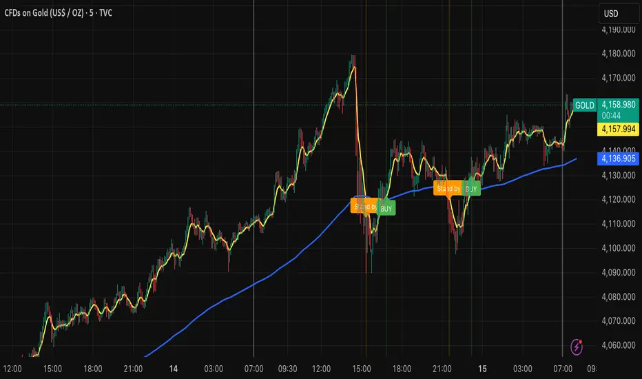
MNQ Morning Indicator | Clean SignalsMNQ Morning Trading Indicator Summary
What It Does
This is a TradingView indicator designed for day trading MNQ (Micro Nasdaq-100 futures) during morning sessions. It generates BUY and SELL signals only when multiple technical conditions align, helping traders identify high-probability trade setups.
Core Strategy
BUY Signal Requirements (All must be true):
✅ Price above VWAP (volume-weighted average price)
✅ Fast EMA (9) above Slow EMA (21) - uptrend confirmation
✅ Price above 15-minute 50 EMA - higher timeframe confirmation
✅ MACD histogram positive - momentum confirmation
✅ RSI above 55 - strength confirmation
✅ ADX above 25 - trending market (not choppy)
✅ Volume 1.5x above average - strong participation
SELL Signal (opposite conditions)
Key Features
🎯 Risk Management
Stop Loss: 2× ATR (Average True Range)
Take Profit 1: 2× ATR (1:2 risk-reward)
Take Profit 2: 3× ATR (1:3 risk-reward)
Dollar values: Calculates P&L based on MNQ's $2/point value
⏰ Session Filter
Default: 9:30 AM - 11:30 AM ET (customizable)
Safety feature: Avoids first 15 minutes (high volatility period)
Won't generate signals outside trading hours
🛡️ Signal Quality
Rates each signal: 🔥 STRONG, ⚡ MEDIUM, or ⚠️ WEAK
Requires minimum 15 bars between signals (prevents overtrading)
📊 Visual Dashboard
Shows real-time metrics:
ATR values
ADX (trend strength)
RSI (momentum)
Market condition (TREND/CHOP)
Session status
Volume status
Signal cooldown timer
Visual Elements
📈 VWAP with standard deviation bands (1σ, 2σ, 3σ)
📉 Multiple EMAs with trend-based coloring
🟢/🔴 Buy/Sell arrows on chart
📋 Detailed trade labels showing entry, SL, TPs, and risk-reward ratios
🎨 Background highlighting for market conditions
Safety Features
Cooldown period between signals
Session restrictions (no trading outside set hours)
First 15-minute avoidance (post-open volatility)
Multi-confirmation requirement (all 7 conditions must align)
Trend filter (ADX minimum to avoid choppy markets)
Best For
Day traders focused on morning sessions
MNQ futures traders
Traders who prefer systematic, rule-based entries
Those wanting pre-calculated risk management levels
Customization
All parameters are adjustable:
EMA periods
MACD settings
RSI thresholds
ADX minimum
ATR multipliers
Session times
Visual preferences
This indicator is designed to be conservative — it waits for strong confirmation before signaling, which means fewer but potentially higher-quality trades.