Primes_3These libraries (Primes_1 -> Primes_4) contain arrays of reduced Prime Numbers to minimize the amount of tokens, allowing more information to be exported.
Values, for example:
7001, 7013, 7019, 7027, 7039, 7043, 7057, 7069, 7079, 7103, 7109, 7021
are reduced to:
7001, 13, 19, 27, 39, 43, 57, 69, 79, 7103, 9, 21
With the restoreValues() function found in the Primes_4 library, the reduced values can be restored back to its original state.
7001, 13, 19, 27, 39, 43, 57, 69, 79, 7103, 9, 21
is restored back to:
7001, 7013, 7019, 7027, 7039, 7043, 7057, 7069, 7079, 7103, 7109, 7021
The libraries contain all Prime Numbers from 2 to 1.340.011
------------------------------------------------------------
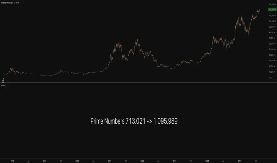
Library "Primes_3"
Prime Numbers 713.021 - 1.095.989
primes_a()
Prime numbers 713.021 - 820.997
primes_b()
Prime numbers 821.003 - 928.979
primes_c()
Prime numbers 929.003 - 1.038.953
primes_d()
Prime numbers 1.039.001 - 1.095.989
Поиск скриптов по запросу "细算江西救护车家长倒赚了四万三+-医疗花费13万(家长视频)++医保报"
Primes_2These libraries (Primes_1 -> Primes_4) contain arrays of reduced Prime Numbers to minimize the amount of tokens, allowing more information to be exported.
Values, for example:
7001, 7013, 7019, 7027, 7039, 7043, 7057, 7069, 7079, 7103, 7109, 7021
are reduced to:
7001, 13, 19, 27, 39, 43, 57, 69, 79, 7103, 9, 21
With the restoreValues() function found in the Primes_4 library, the reduced values can be restored back to its original state.
7001, 13, 19, 27, 39, 43, 57, 69, 79, 7103, 9, 21
is restored back to:
7001, 7013, 7019, 7027, 7039, 7043, 7057, 7069, 7079, 7103, 7109, 7021
The libraries contain all Prime Numbers from 2 to 1.340.011
------------------------------------------------------------
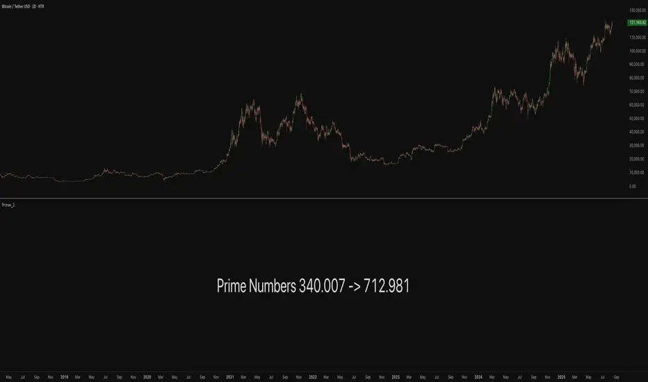
Library "Primes_2"
Prime Numbers 340.007 - 712.981
primes_a()
Prime numbers 340.007 - 441.971
primes_b()
Prime numbers 442.003 - 545.959
primes_c()
Prime numbers 546.001 - 650.987
primes_d()
Prime numbers 651.017 - 712.981
Primes_1These libraries (Primes_1 -> Primes_4) contain arrays of reduced Prime Numbers to minimize the amount of tokens, allowing more information to be exported.
Values, for example:
7001, 7013, 7019, 7027, 7039, 7043, 7057, 7069, 7079, 7103, 7109, 7021
are reduced to:
7001, 13, 19, 27, 39, 43, 57, 69, 79, 7103, 9, 21
With the restoreValues() function found in the Primes_4 library, the reduced values can be restored back to its original state.
7001, 13, 19, 27, 39, 43, 57, 69, 79, 7103, 9, 21
is restored back to:
7001, 7013, 7019, 7027, 7039, 7043, 7057, 7069, 7079, 7103, 7109, 7021
The libraries contain all Prime Numbers from 2 to 1.340.011
------------------------------------------------------------
Library "Primes_1"
Prime Numbers 2 - 339.991
primes_a()
Prime numbers 2 - 81.689
primes_b()
Prime numbers 81.701 - 175.897
primes_c()
Prime numbers 175.909 - 273.997
primes_d()
Prime numbers 274.007 - 339.991

Wolf Exit Oscillator Enhanced
# Wolf Exit Oscillator Enhanced
## What it is (quick take)
**Wolf Exit Oscillator Enhanced** is a clean, rules-first **exit timing tool** built on the **True Strength Index (TSI)** with two optional safeguards:
1. **Signal-line crossover** (to avoid bailing on shallow dips), and
2. **EMA confirmation** (price-based “is the trend actually weakening/strengthening?” check).
Use it to standardize when you **take profits, cut losers, or scale out**—especially after momentum runs hot or cold.
> Works best **paired** with:
>
> * **ABS NR — Fail-Safe Confirm (v4.2.2)** for entries
> * **ABS Companion Oscillator — Trend / Exhaustion / New Trend** for trend/exhaustion context
---
## How to use it (operational workflow)
1. **Set your bands**
* `exitHigh` and `exitLow` mark “overcooked” zones on the TSI scale (default: +60 / –60).
* Above `exitHigh` = momentum stretched **up** (good place to **exit shorts** or **take long profits**).
* Below `exitLow` = momentum stretched **down** (good place to **exit longs** or **take short profits**).
2. **Choose strictness**
* **Base mode**: the moment TSI crosses out of a band, you get an exit signal.
* **Add Signal-Line Cross** (`enableSignalX = true`): require TSI to cross its signal in the same direction → **fewer, cleaner exits**.
* **Add EMA Filter** (`enableEMAFilter = true`): also require **price** to confirm (e.g., long exit only if price < EMA). This avoids bailing during healthy trends.
3. **Execute with structure**
* **Full exit** when a signal fires, or
* **Scale out** (e.g., 50% on first signal, remainder on trail/secondary signal), or
* **Move stop** to lock gains once an exit signal prints.
4. **Alerts**
* Set to **“Once per bar close”** to avoid intrabar flip-flop.
* Use the two provided alert names for automation (see “Alerts” below).
---
## Signals & visuals
* **TSI line** (solid) and **Signal line** (dashed) with optional **histogram** (TSI − Signal).
* **Horizontal bands** at `exitHigh` and `exitLow`.
* **Labels**:
* **Exit Long** appears when long-side momentum breaks down (below `exitLow`, plus any enabled filters).
* **Exit Short** appears when short-side momentum breaks down (above `exitHigh`, plus any enabled filters).
**Alerts (stable names):**
* **WolfExit — Exit Long**
* **WolfExit — Exit Short**
---
## Non-repainting behavior (what to expect)
* The oscillator is computed with **EMAs on current timeframe**—no higher-timeframe lookahead, no repaint.
* **Intrabar**: TSI/Signal can fluctuate; use **bar-close evaluation** (and alert setting “Once per bar close”) to lock signals.
* If you enable the EMA filter, that check is also evaluated at bar close.
---
## Every input explained (and how changing it alters behavior)
### Momentum engine (TSI)
* **TSI Long EMA Length (`tsiLongLen`, default 25)**
Higher = smoother, slower momentum; fewer signals. Lower = twitchier, more signals.
* **TSI Short EMA Length (`tsiShortLen`, default 13)**
Fine-tunes responsiveness on top of the long length. Lower short → snappier TSI.
* **TSI Signal Line Length (`tsisigLen`, default 7)**
Higher = slower signal line (harder to cross) → fewer signals. Lower = easier crosses → more signals.
### Thresholds (the bands)
* **Exit Threshold High (`exitHigh`, default +60)**
Raise to demand **stronger** overbought before signaling short exits / long profit-takes. Lower to trigger sooner.
* **Exit Threshold Low (`exitLow`, default −60)**
Raise (toward 0) to trigger **earlier** on longs; lower (more negative) to wait for deeper downside stretch.
### Confirmation layers
* **Require Signal Line Crossover (`enableSignalX`, default true)**
On = TSI must cross its signal (same direction as exit) → **filters out shallow wiggles**. Off = faster, more frequent exits.
* **Enable EMA Confirmation Filter (`enableEMAFilter`, default true)**
On = require **price < EMA** for **Exit Long** and **price > EMA** for **Exit Short**.
* **EMA Exit Confirmation Length (`exitEMALen`, default 50)**
Higher = **trendier** filter (harder to flip) → fewer exits; Lower = more reactive → more exits.
### Visuals
* **Show Histogram (`showHist`)**
On = quick visual for TSI–Signal spread (helps spot weakening momentum before a cross).
* **Plot Exit Signals (`showSignals`)**
Toggle labels if you only want the lines/bands with alerts.
---
## Tuning recipes (quick, practical)
* **Strong trend days (avoid premature exits)**
* Keep **`enableSignalX = true`** and **`enableEMAFilter = true`**
* Increase **`exitEMALen`** (e.g., 80)
* Consider raising **`exitHigh`** to 65–70 (and lowering **`exitLow`** to −65/−70)
* **Choppy/range days (exit faster, take the cash)**
* **`enableEMAFilter = false`** (don’t wait for price filter)
* **`enableSignalX`** optional; try off for quicker responses
* Bring bands closer to **±50** to take profits earlier
* **Scalping / lower timeframes**
* Shorten **TSI lengths** a bit (e.g., 21/9/5)
* Consider **`exitHigh=55 / exitLow=-55`**
* Keep **histogram on** to visualize momentum flip risk
* **Swing trading / higher timeframes**
* Lengthen **TSI** (e.g., 35/21/9) and **`exitEMALen`** (e.g., 100)
* Wider bands (±65 to ±75) to catch bigger moves before exiting
---
## Playbooks (how to actually trade it)
* **Entry from ABS NR FS, exit with Wolf**
* Take entries from **ABS NR — Fail-Safe Confirm** (triangle).
* Use **Wolf Exit** to scale out: 50% on first exit label, trail remainder with price/EMA or your stop logic.
* **Pyramid & protect**
* Add on re-accelerations (TSI pulls back toward zero without breaching the opposite band).
* The first **Exit** signal → take partial, raise stop to last higher low / lower high.
* **Mean-reversion fade management**
* When fading with ABS NR (KC band pokes + stretched |Z|), target the first opposite **Exit** signal as your “don’t overstay” cue.
---
## Suggested starting points
* **Day trading (5–15m):**
* TSI: **25 / 13 / 7** (default)
* Bands: **+60 / −60**
* Confirmations: **SignalX = on**, **EMA Filter = on**, **EMA Len = 50**
* Alerts: **Once per bar close**
* **Scalping (1–3m):**
* TSI: **21 / 9 / 5**
* Bands: **±55**
* Confirmations: **SignalX = on**, **EMA Filter = off** (optional for speed)
* **Swing (1h–D):**
* TSI: **35 / 21 / 9**
* Bands: **+65 / −65** (or ±70)
* Confirmations: **SignalX = on**, **EMA Filter = on**, **EMA Len = 100**
---
## Best-practice pairings
* **Entries:** **ABS NR — Fail-Safe Confirm (v4.2.2)**
* Take ABS triangles; let Wolf standardize exits so you’re not guessing.
* **Context:** **ABS Companion Oscillator**
* Prefer holding longer when the companion stays above (for longs) or below (for shorts) its neutral band and **no EXH tag** prints.
* If companion flags **EXH** against your position, tighten stops; Wolf’s next exit signal becomes high priority.
---
## Notes & disclaimers
* This is an **exit signal tool**, not a strategy or broker.
* Signals are strongest when aligned with your **entry logic** and a **risk framework** (position sizing, stops, partials).
* All evaluations are **current timeframe**; no higher-timeframe lookahead is used.
* Markets change—tune the bands and confirmations per symbol/timeframe.
---
**Tip:** Keep your alerts simple—one for **Exit Long**, one for **Exit Short**, **Once per bar close**. Use partial exits on the first signal, and let your stop/trailing logic handle the rest.

ADR/ATR Session by LK## **Features**
1. **Custom ADR & ATR Calculation**
* Calculates **Average Daily Range (ADR)** and **Average True Range (ATR)** separately for:
* **Session timeframe** (default H4 / 06:00–13:00)
* **Daily timeframe**
* Independent smoothing method selection (**SMA, EMA, RMA, WMA**) for H4 ADR, H4 ATR, Daily ADR, and Daily ATR.
2. **Percentage Metrics**
* % of ADR / ATR covered by the **current H4 bar**.
* ADR / ATR expressed as a percentage of the **current price**.
* % of ADR already reached for the **current day**.
* % of Daily ATR vs current day’s True Range.
3. **Dynamic Chart Lines**
* Draws **3 lines for H4**: Session Open, ADR High, ADR Low.
* Draws **3 lines for Daily**: Daily Open, ADR High, ADR Low.
* Lines **extend to the right** so they stay visible across the chart.
* Colors and widths are fully customizable.
4. **Real-Time Data Table**
* Compact table displaying all ADR/ATR values and percentages.
* Adjustable table font size (**tiny, small, normal, large, huge**).
* Transparent background option for minimal chart obstruction.
5. **Flexible Session Settings**
* Select session start and end time in hours/minutes.
* Choose session timezone (chart timezone or major financial centers).
* Toggle H4 lines, Daily lines separately.
6. **Lookahead Control**
* Option to wait for higher-timeframe candle close before updating values (more accurate, less repainting).
---
## **How to Use**
### **1. Adding the Indicator**
* Copy and paste the Pine Script into TradingView’s Pine Editor.
* Click **“Add to chart”**.
* Make sure your chart supports the higher timeframes you choose (e.g., H4 and Daily).
### **2. Setting Your Session**
* **Session Start Hour** & **End Hour** → Defines the intraday session to measure ADR/ATR (default: 06:00–13:00).
* **Session Timezone** → Pick “Chart” or a major financial center (e.g., New York, London, Tokyo).
### **3. Choosing Smoothing Methods**
* For each ADR/ATR (H4 and Daily), choose:
* SMA (Simple)
* EMA (Exponential)
* RMA (Wilder’s smoothing)
* WMA (Weighted)
### **4. Adjusting Chart Display**
* **Show H4 Lines** → Displays session open and ADR High/Low for the current H4 session.
* **Show Daily Lines** → Displays daily open and ADR High/Low.
* Customize line colors and widths.
### **5. Reading the Table**
* **H4 Section**
* ADR / ATR values for the selected session.
* % of ADR/ATR covered by the **current H4 bar**.
* ADR/ATR as % of the current price.
* **Daily Section**
* ADR / ATR for the daily timeframe.
* % of ADR already covered by today’s range.
* ADR/ATR as % of price.
### **6. Pro Tips**
* Use **H4 ADR %** to gauge intraday exhaustion — if current range is near 100%, market may slow or reverse.
* Use **Daily ADR %** for swing trade context — if a day has moved beyond its ADR, expect lower continuation probability.
* Combine with support/resistance to identify high-probability reversal zones.

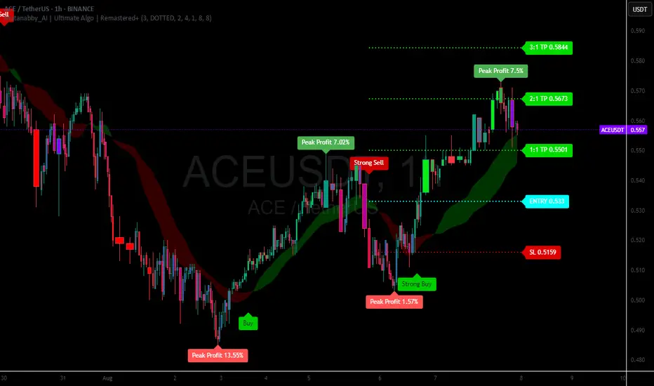
Mutanabby_AI | Ultimate Algo | Remastered+Overview
The Mutanabby_AI Ultimate Algo Remastered+ represents a sophisticated trend-following system that combines Supertrend analysis with multiple moving average confirmations. This comprehensive indicator is designed specifically for identifying high-probability trend continuation and reversal opportunities across various market conditions.
Core Algorithm Components
**Supertrend Foundation**: The primary signal generation relies on a customizable Supertrend indicator with adjustable sensitivity (1-20 range). This adaptive trend-following tool uses Average True Range calculations to establish dynamic support and resistance levels that respond to market volatility.
**SMA Confirmation Matrix**: Multiple Simple Moving Averages (SMA 4, 5, 9, 13) provide layered confirmation for signal strength. The algorithm distinguishes between regular signals and "Strong" signals based on SMA 4 vs SMA 5 relationship, offering traders different conviction levels for position sizing.
**Trend Ribbon Visualization**: SMA 21 and SMA 34 create a visual trend ribbon that changes color based on their relationship. Green ribbon indicates bullish momentum while red signals bearish conditions, providing immediate visual trend context.
**RSI-Based Candle Coloring**: Advanced 61-tier RSI system colors candles with gradient precision from deep red (RSI ≤20) through purple transitions to bright green (RSI ≥79). This visual enhancement helps traders instantly assess momentum strength and overbought/oversold conditions.
Signal Generation Logic
**Buy Signal Criteria**:
- Price crosses above Supertrend line
- Close price must be above SMA 9 (trend confirmation)
- Signal strength determined by SMA 4 vs SMA 5 relationship
- "Strong Buy" when SMA 4 ≥ SMA 5
- Regular "Buy" when SMA 4 < SMA 5
**Sell Signal Criteria**:
- Price crosses below Supertrend line
- Close price must be below SMA 9 (trend confirmation)
- Signal strength based on SMA relationship
- "Strong Sell" when SMA 4 ≤ SMA 5
- Regular "Sell" when SMA 4 > SMA 5
Advanced Risk Management System
**Automated TP/SL Calculation**: The indicator automatically calculates stop loss and take profit levels using ATR-based measurements. Risk percentage and ATR length are fully customizable, allowing traders to adapt to different market conditions and personal risk tolerance.
**Multiple Take Profit Targets**:
- 1:1 Risk-Reward ratio for conservative profit taking
- 2:1 Risk-Reward for balanced trade management
- 3:1 Risk-Reward for maximum profit potential
**Visual Risk Display**: All risk management levels appear as both labels and optional trend lines on the chart. Customizable line styles (solid, dashed, dotted) and positioning ensure clear visualization without chart clutter.
**Dynamic Level Updates**: Risk levels automatically recalculate with each new signal, maintaining current market relevance throughout position lifecycles.
Visual Enhancement Features
**Customizable Display Options**: Toggle trend ribbon, TP/SL levels, and risk lines independently. Decimal precision adjustments (1-8 decimal places) accommodate different instrument price formats and personal preferences.
**Professional Label System**: Clean, informative labels show entry points, stop losses, and take profit targets with precise price levels. Labels automatically position themselves for optimal chart readability.
**Color-Coded Momentum**: The gradient RSI candle coloring system provides instant visual feedback on momentum strength, helping traders assess market energy and potential reversal zones.
Implementation Strategy
**Timeframe Optimization**: The algorithm performs effectively across multiple timeframes, with higher timeframes (4H, Daily) providing more reliable signals for swing trading. Lower timeframes work well for day trading with appropriate risk adjustments.
**Sensitivity Adjustment**: Lower sensitivity values (1-5) generate fewer but higher-quality signals, ideal for conservative approaches. Higher sensitivity (15-20) increases signal frequency for active trading styles.
**Risk Management Integration**: Use the automated risk calculations as baseline parameters, adjusting risk percentage based on account size and market conditions. The 1:1, 2:1, 3:1 targets enable systematic profit-taking strategies.
Market Application
**Trend Following Excellence**: Primary strength lies in capturing significant trend movements through the Supertrend foundation with SMA confirmation. The dual-layer approach reduces false signals common in single-indicator systems.
**Momentum Assessment**: RSI-based candle coloring provides immediate momentum context, helping traders assess signal strength and potential continuation probability.
**Range Detection**: The trend ribbon helps identify ranging conditions when SMA 21 and SMA 34 converge, alerting traders to potential breakout opportunities.
Performance Optimization
**Signal Quality**: The requirement for both Supertrend crossover AND SMA 9 confirmation significantly improves signal reliability compared to basic trend-following approaches.
**Visual Clarity**: The comprehensive visual system enables rapid market assessment without complex calculations, ideal for traders managing multiple instruments.
**Adaptability**: Extensive customization options allow fine-tuning for specific markets, trading styles, and risk preferences while maintaining the core algorithm integrity.
## Non-Repainting Design
**Educational Note**: This indicator uses standard TradingView functions (Supertrend, SMA, RSI) with normal behavior patterns. Real-time updates on current candles are expected and standard across all technical indicators. Historical signals on closed candles remain fixed and unchanged, ensuring reliable backtesting and analysis.
**Signal Confirmation**: Final signals are confirmed only when candles close, following standard technical analysis principles. The algorithm provides clear distinction between developing signals and confirmed entries.
Technical Specifications
**Supertrend Parameters**: Default sensitivity of 4 with ATR length of 11 provides balanced signal generation. Sensitivity range from 1-20 allows adaptation to different market volatilities and trading preferences.
**Moving Average Configuration**: SMA periods of 8, 9, and 13 create multi-layered trend confirmation, while SMA 21 and 34 form the visual trend ribbon for broader market context.
**Risk Management**: ATR-based calculations with customizable risk percentage ensure dynamic adaptation to market volatility while maintaining consistent risk exposure principles.
Recommended Settings
**Conservative Approach**: Sensitivity 4-5, RSI length 14, higher timeframes (4H, Daily) for swing trading with maximum signal reliability.
**Active Trading**: Sensitivity 6-8, RSI length 8-10, intermediate timeframes (1H) for balanced signal frequency and quality.
**Scalping Setup**: Sensitivity 10-15, RSI length 5-8, lower timeframes (15-30min) with enhanced risk management protocols.
## Conclusion
The Mutanabby_AI Ultimate Algo Remastered+ combines proven trend-following principles with modern visual enhancements and comprehensive risk management. The algorithm's strength lies in its multi-layered confirmation approach and automated risk calculations, providing both novice and experienced traders with clear signals and systematic trade management.
Success with this system requires understanding the relationship between signal strength indicators and adapting sensitivity settings to match current market conditions. The comprehensive visual feedback system enables rapid decision-making while the automated risk management ensures consistent trade parameters.
Practice with different sensitivity settings and timeframes to optimize performance for your specific trading style and risk tolerance. The algorithm's systematic approach provides an excellent framework for disciplined trend-following strategies across various market environments.
5 SMA/EMA and Zigzag- Chỉ báo gộp của 2 chỉ báo 5 đường MA/EMA/WMA và đường zigzag
- Các thông số đường EMA và zigzag mặc định đã được đặt theo thông số khoá học Fibo
- 5 đường MA có thể lựa chọn loại đường SMA, EMA, WMA, VWM và được bật mặc định 3 đường EMA 8, 13, 21 và có thể thay đổi màu đường định dạng đường. Và giao cắt của đường EMA 10 và 21 được đánh dấu bằng các dấu chấm tròn.
- Đường zigzag được đặt thông số mặc định là 3.
Màu đường và độ dày đường zigzag có thể thay đổi từ bảng lựa chọn, kiểu đường thì phải thay đổi trong code.
- Bảng giá trị RSI, MA RSI thì đang để 7 khung thời gian. Muốn tắt bớt thì phải tắt trong code
Và giá trị của RSI và MA RSI sẽ không đúng với các Tf 5, 15, 30 nếu Tf của chart lớn hơn TF này (do tradingview) . Vd TF chart là 15m thì giá trị RSI trong bảng của khung 5m không đúng, Tf chart là 60m thì giá trị RSI của 30m, 15m , 5m trong bảng là không đúng. TF chart là 4H thì giá trị trong bảng của khung 5m, 15m 30m không đúng, còn giá trị của 1H, 2H, 3H vẫn đúng.
This is a combined indicator of two separate indicators: a 5-line MA/EMA/WMA indicator and a ZigZag indicator.
The default parameters for the EMA and ZigZag lines are set according to the Fibo course settings.
For the 5 moving averages, you can choose between SMA, EMA, WMA, and VWM. By default, 3 EMA lines (8, 13, 21) are enabled, and their colors and styles can be customized. The crossover between EMA 10 and EMA 21 is marked with circular dots.
The default setting for the ZigZag line is 3.
The color and thickness of the ZigZag line can be changed via the input panel, but the line style must be modified in the code.
The RSI and MA RSI value table is currently set to display across 7 timeframes. To reduce the number of timeframes shown, you will need to edit the code manually.
Note: The RSI and MA RSI values will not be accurate for timeframes 5m, 15m, and 30m if the chart's timeframe is higher than these (due to limitations in TradingView).
For example:
If the chart is on 15m, the RSI value for the 5m frame in the table will be incorrect.
If the chart is on 60m, then RSI values for 30m, 15m, and 5m will be incorrect.
If the chart is on 4H, the RSI values for 5m, 15m, and 30m will be incorrect, but the values for 1H, 2H, and 3H will still be correct.

7 EMA CloudThe "7 EMA Cloud" script was likely flagged because it reuses the core concept of EMA clouds (shading areas between multiple EMAs to visualize trends, support/resistance, and momentum) without crediting the original inventor, Ripster (author ripster47 on TradingView). This concept is prominently associated with Ripster's "EMA Clouds" indicator, which popularized filling spaces between EMA pairs for trading signals. TradingView's house rules require crediting authors when reusing open-source ideas or code, even if not a direct copy-paste, and mandate significant improvements where the original forms a small proportion of the script. Your version adds features like multiple color modes (Classic rainbow, Monochrome, Heatmap), customizable signal sizes, and crossover alerts between the first and last EMA, which are enhancements, but the foundational EMA ribbon/cloud idea needs explicit attribution in the description and ideally code comments to comply.
Additionally, the description might be seen as not fully self-contained (e.g., it uses promotional language like "Advanced" and "Adaptive Trend & Signal Suite" without deeply explaining calculations or use cases), potentially violating rules against relying on code or external references for clarity.
To fix this, republish a new version with proper credits, ensure the description is detailed and standalone, and emphasize your improvements (e.g., the 7 Fibonacci-based EMAs, color modes, and signals). Do not reuse the flagged script—create a fresh one. Here's a compliant description you can use:
7 EMA Cloud Indicator
Overview
The 7 EMA Cloud overlays seven exponential moving averages (EMAs) with Fibonacci-inspired periods and fills the spaces between them with customizable "clouds" to visually represent trend strength, direction, and convergence/divergence. It includes crossover signals between the shortest and longest EMAs for potential entry/exit points, with adjustable visual modes for different trading styles. This helps traders identify bullish/bearish momentum, support/resistance zones, and overextensions in trending or ranging markets.
This script builds on the EMA cloud concept popularized by Ripster (ripster47) in their "EMA Clouds" indicatortradingview.com, where areas between EMA pairs are shaded for trend analysis. Improvements include a fixed set of 7 Fibonacci EMAs, multiple color schemes (Classic rainbow, Monochrome grayscale, Heatmap for intensity), user-selectable signal sizes, and transparency controls. Released under the Mozilla Public License 2.0.
Key Features
7 EMAs with Clouds: EMAs at periods 8, 13, 21, 34, 55, 89, and 144; clouds filled between consecutive pairs to show alignment (tight clouds for consolidation, wide for trends).
Color Modes:
Classic: Rainbow gradients (blue to purple) for vibrant distinction.
Monochrome: Grayscale shades for minimalistic charts.
Heatmap: Red-to-blue spectrum to highlight "hot" (volatile) vs. "cool" (stable) areas.
Crossover Signals: Triangle markers (up for bullish, down for bearish) when the shortest EMA crosses the longest; sizes from Tiny to Huge.
Display Options: Toggle EMA lines on/off, adjust cloud transparency (0-100%), and enable alerts for crossovers.
Alerts: Notifications for "Bullish EMA Crossover" (EMA1 > EMA7) and "Bearish EMA Crossover" (EMA1 < EMA7).
How It Works
EMA Calculations: Each EMA is computed using ta.ema(close, period), with periods based on Fibonacci sequences for natural market rhythm alignment.
Clouds: Filled via fill() between plot pairs, with colors derived from the selected mode and transparency applied.
Signals: Detected with ta.crossover(ema1, ema7) and ta.crossunder(ema1, ema7), plotted as shapes with mode-specific colors (e.g., green/lime for bull, red for bear).
Customization: Inputs grouped into EMA Settings (periods), Display Settings (visibility, colors, transparency), and Signal Settings (size).
Customization Options
EMA Periods: Individually adjustable (defaults: 8, 13, 21, 34, 55, 89, 144).
Show EMAs: Toggle to hide lines and focus on clouds.
Cloud Transparency: 0% for solid fills, 100% for invisible (default 80%).
Color Mode: Switch between Classic, Monochrome, or Heatmap.
Signal Size: Tiny, Small, Normal, Large, or Huge for crossover markers.
Ideal Use Case
Suited for swing or trend-following on any timeframe (e.g., 15m-1h for intraday, daily for swings) and assets (stocks, forex, crypto, futures). Enter long on bullish crossovers above aligned clouds; exit on bearish signals or cloud widenings. Use Monochrome for clean charts or Heatmap for volatility emphasis. Combine with volume or RSI for confirmation.
Why It's Valuable
By expanding Ripster's EMA cloud idea with multi-mode visuals and integrated signals, this indicator provides a versatile, at-a-glance tool for trend assessment—reducing noise while highlighting key shifts. It's more adaptive than basic MA ribbons, with Fibonacci periods adding a layer of harmonic analysis.
Note: Test on historical data or demo accounts. Not financial advice—incorporate risk management. Optimized for Pine Script v5; some features may vary on non-overlay charts.

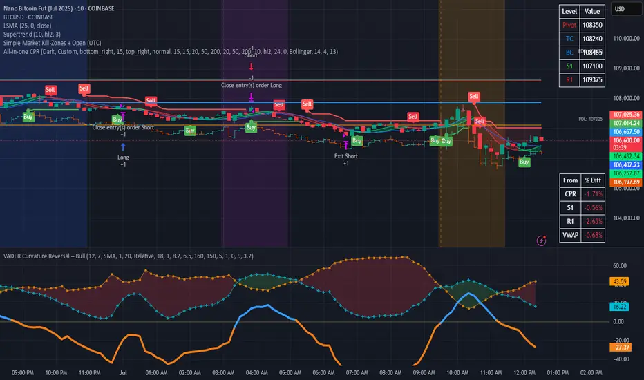
Simple Market Kill-Zones + Open (UTC)What it does
This Pine v6 indicator highlights the “kill-zones” around the big session opens—Asian (23:00–03:00 UTC), London (07:00–09:00 UTC) and New York (13:30–15:30 UTC)—by reading each bar’s actual UTC timestamp. It also draws dashed vertical lines at exactly 23:00, 07:00 and 13:30 UTC, so you never miss the liquidity ramps. Because it uses raw UTC hours/minutes, it stays accurate even when exchanges pause (e.g. Nano-BTC’s daily halt) or your chart’s display timezone changes.
Key Inputs
Show Asia/London/NY Kill Zone – toggle each shaded band on/off
Zone Colors – pick your own semi-transparent hues
Show Session-Open Lines – enable dashed verticals at the exact open times
Line Colors – customize the line opacity and style
How to use
Apply on your favorite timeframe (15 min–1 h is a sweet spot).
Toggle the zones you care about and pick readable colors.
Use the dashed lines as entry triggers or as visual bookmarks.
In your own Pine strategies, wrap order logic with the zone booleans to only trade when liquidity’s alive.
Options Strategy V1.3📈 Options Strategy V1.3 — EMA Crossover + RSI + ATR + Opening Range
Overview:
This strategy is designed for short-term directional trades on large-cap stocks or ETFs, especially when trading options. It combines classic trend-following signals with momentum confirmation, volatility-based risk management, and session timing filters to help identify high-probability entries with predefined stop-loss and profit targets.
🔍 Strategy Components:
EMA Crossover (Fast/Slow)
Entry signals are triggered by the crossover of a short EMA above or below a long EMA — a traditional trend-following method to detect shifts in momentum.
RSI Filter
RSI confirms the signal by avoiding entries in overbought/oversold zones unless certain momentum conditions are met.
Long entry requires RSI ≥ Long Threshold
Short entry requires RSI ≤ Short Threshold
ATR-Based SL & TP
Stop-loss is set dynamically as a multiple of ATR below (long) or above (short) the entry price.
Take-profit is placed as a ratio (TP/SL) of the stop distance, ensuring consistent reward/risk structure.
Opening Range Filter (Optional)
If enabled, the strategy only triggers trades after price breaks out of the 09:30–09:45 EST range, ensuring participation in directional moves.
Session Filters
No trades from 04:00 to 09:30 and from 16:00 to 20:00 EST, avoiding low-liquidity periods.
All open trades are closed at 15:55 EST, to avoid overnight risk or expiration issues for options.
⚙️ Built-in Presets:
You can choose one of the built-in ticker-specific presets for optimal conditions:
Ticker EMAs RSI (Long/Short) ATR SL×ATR TP/SL
SPY 8/28 56 / 26 14 1.4× 4.0×
TSLA 23/27 56 / 33 13 1.4× 3.6×
AAPL 6/13 61 / 26 23 1.4× 2.1×
MSFT 25/32 54 / 26 14 1.2× 2.2×
META 25/32 53 / 26 17 1.8× 2.3×
AMZN 28/32 55 / 25 16 1.8× 2.3×
You can also choose "Custom" to fully configure all parameters to your own market and strategy preferences.
📌 Best Use Case:
This strategy is especially suited for intraday options trading, where timing and risk control are critical. It works best on liquid tickers with strong trends or clear breakout behavior.

The Sequences of FibonacciThe Sequences of Fibonacci - Advanced Multi-Timeframe Confluence Analysis System
THEORETICAL FOUNDATION & MATHEMATICAL INNOVATION
The Sequences of Fibonacci represents a revolutionary approach to market analysis that synthesizes classical Fibonacci mathematics with modern adaptive signal processing. This indicator transcends traditional Fibonacci retracement tools by implementing a sophisticated multi-dimensional confluence detection system that reveals hidden market structure through mathematical precision.
Core Mathematical Framework
Dynamic Fibonacci Grid System:
Unlike static Fibonacci tools, this system calculates highest highs and lowest lows across true Fibonacci sequence periods (8, 13, 21, 34, 55 bars) creating a dynamic grid of mathematical support and resistance levels that adapt to market structure in real-time.
Multi-Dimensional Confluence Detection:
The engine employs advanced mathematical clustering algorithms to identify areas where multiple derived Fibonacci retracement levels (0.382, 0.500, 0.618) from different timeframe perspectives converge. These "Confluence Zones" are mathematically classified by strength:
- CRITICAL Zones: 8+ converging Fibonacci levels
- HIGH Zones: 6-7 converging levels
- MEDIUM Zones: 4-5 converging levels
- LOW Zones: 3+ converging levels
Adaptive Signal Processing Architecture:
The system implements adaptive Stochastic RSI calculations with dynamic overbought/oversold levels that adjust to recent market volatility rather than using fixed thresholds. This prevents false signals during changing market conditions.
COMPREHENSIVE FEATURE ARCHITECTURE
Quantum Field Visualization System
Dynamic Price Field Mathematics:
The Quantum Field creates adaptive price channels based on EMA center points and ATR-based amplitude calculations, influenced by the Unified Field metric. This visualization system helps traders understand:
- Expected price volatility ranges
- Potential overextension zones
- Mathematical pressure points in market structure
- Dynamic support/resistance boundaries
Field Amplitude Calculation:
Field Amplitude = ATR × (1 + |Unified Field| / 10)
The system generates three quantum levels:
- Q⁰ Level: 0.618 × Field Amplitude (Primary channel)
- Q¹ Level: 1.0 × Field Amplitude (Secondary boundary)
- Q² Level: 1.618 × Field Amplitude (Extreme extension)
Advanced Market Analysis Dashboard
Unified Field Analysis:
A composite metric combining:
- Price momentum (40% weighting)
- Volume momentum (30% weighting)
- Trend strength (30% weighting)
Market Resonance Calculation:
Measures price-volume correlation over 14 periods to identify harmony between price action and volume participation.
Signal Quality Assessment:
Synthesizes Unified Field, Market Resonance, and RSI positioning to provide real-time evaluation of setup potential.
Tiered Signal Generation Logic
Tier 1 Signals (Highest Conviction):
Require ALL conditions:
- Adaptive StochRSI setup (exiting dynamic OB/OS levels)
- Classic StochRSI divergence confirmation
- Strong reversal bar pattern (adaptive ATR-based sizing)
- Level rejection from Confluence Zone or Fibonacci level
- Supportive Unified Field context
Tier 2 Signals (Enhanced Opportunity Detection):
Generated when Tier 1 conditions aren't met but exceptional circumstances exist:
- Divergence candidate patterns (relaxed divergence requirements)
- Exceptionally strong reversal bars at critical levels
- Enhanced level rejection criteria
- Maintained context filtering
Intelligent Visualization Features
Fractal Matrix Grid:
Multi-layer visualization system displaying:
- Shadow Layer: Foundational support (width 5)
- Glow Layer: Core identification (width 3, white)
- Quantum Layer: Mathematical overlay (width 1, dotted)
Smart Labeling System:
Prevents overlap using ATR-based minimum spacing while providing:
- Fibonacci period identification
- Topological complexity classification (0, I, II, III)
- Exact price levels
- Strength indicators (○ ◐ ● ⚡)
Wick Pressure Analysis:
Dynamic visualization showing momentum direction through:
- Multi-beam projection lines
- Particle density effects
- Progressive transparency for natural flow
- Strength-based sizing adaptation
PRACTICAL TRADING IMPLEMENTATION
Signal Interpretation Framework
Entry Protocol:
1. Confluence Zone Approach: Monitor price approaching High/Critical confluence zones
2. Adaptive Setup Confirmation: Wait for StochRSI to exit adaptive OB/OS levels
3. Divergence Verification: Confirm classic or candidate divergence patterns
4. Reversal Bar Assessment: Validate strong rejection using adaptive ATR criteria
5. Context Evaluation: Ensure Unified Field provides supportive environment
Risk Management Integration:
- Stop Placement: Beyond rejected confluence zone or Fibonacci level
- Position Sizing: Based on signal tier and confluence strength
- Profit Targets: Next significant confluence zone or quantum field boundary
Adaptive Parameter System
Dynamic StochRSI Levels:
Unlike fixed 80/20 levels, the system calculates adaptive OB/OS based on recent StochRSI range:
- Adaptive OB: Recent minimum + (range × OB percentile)
- Adaptive OS: Recent minimum + (range × OS percentile)
- Lookback Period: Configurable 20-100 bars for range calculation
Intelligent ATR Adaptation:
Bar size requirements adjust to market volatility:
- High Volatility: Reduced multiplier (bars naturally larger)
- Low Volatility: Increased multiplier (ensuring significance)
- Base Multiplier: 0.6× ATR with adaptive scaling
Optimization Guidelines
Timeframe-Specific Settings:
Scalping (1-5 minutes):
- Fibonacci Rejection Sensitivity: 0.3-0.8
- Confluence Threshold: 2-3 levels
- StochRSI Lookback: 20-30 bars
Day Trading (15min-1H):
- Fibonacci Rejection Sensitivity: 0.5-1.2
- Confluence Threshold: 3-4 levels
- StochRSI Lookback: 40-60 bars
Swing Trading (4H-1D):
- Fibonacci Rejection Sensitivity: 1.0-2.0
- Confluence Threshold: 4-5 levels
- StochRSI Lookback: 60-80 bars
Asset-Specific Optimization:
Cryptocurrency:
- Higher rejection sensitivity (1.0-2.5) for volatile conditions
- Enable Tier 2 signals for increased opportunity detection
- Shorter adaptive lookbacks for rapid market changes
Forex Major Pairs:
- Moderate sensitivity (0.8-1.5) for stable trending
- Focus on Higher/Critical confluence zones
- Longer lookbacks for institutional flow detection
Stock Indices:
- Conservative sensitivity (0.5-1.0) for institutional participation
- Standard confluence thresholds
- Balanced adaptive parameters
IMPORTANT USAGE CONSIDERATIONS
Realistic Performance Expectations
This indicator provides probabilistic advantages based on mathematical confluence analysis, not guaranteed outcomes. Signal quality varies with market conditions, and proper risk management remains essential regardless of signal tier.
Understanding Adaptive Features:
- Adaptive parameters react to historical data, not future market conditions
- Dynamic levels adjust to past volatility patterns
- Signal quality reflects mathematical alignment probability, not certainty
Market Context Awareness:
- Strong trending markets may produce fewer reversal signals
- Range-bound conditions typically generate more confluence opportunities
- News events and fundamental factors can override technical analysis
Educational Value
Mathematical Concepts Introduced:
- Multi-dimensional confluence analysis
- Adaptive signal processing techniques
- Dynamic parameter optimization
- Mathematical field theory applications in trading
- Advanced Fibonacci sequence applications
Skill Development Benefits:
- Understanding market structure through mathematical lens
- Recognition of multi-timeframe confluence principles
- Appreciation for adaptive vs. static analysis methods
- Integration of classical Fibonacci with modern signal processing
UNIQUE INNOVATIONS
First-Ever Implementations
1. True Fibonacci Sequence Periods: First indicator using authentic Fibonacci numbers (8,13,21,34,55) for timeframe analysis
2. Mathematical Confluence Clustering: Advanced algorithm identifying true Fibonacci level convergence
3. Adaptive StochRSI Boundaries: Dynamic OB/OS levels replacing fixed thresholds
4. Tiered Signal Architecture: Democratic signal weighting with quality classification
5. Quantum Field Price Visualization: Mathematical field representation of price dynamics
Visualization Breakthroughs
- Multi-Layer Fibonacci Grid: Three-layer rendering with intelligent spacing
- Dynamic Confluence Zones: Strength-based color coding and sizing
- Adaptive Parameter Display: Real-time visualization of dynamic calculations
- Mathematical Field Effects: Quantum-inspired price channel visualization
- Progressive Transparency Systems: Natural visual flow without chart clutter
COMPREHENSIVE DASHBOARD SYSTEM
Multi-Size Display Options
Small Dashboard: Core metrics for mobile/limited screen space
Normal Dashboard: Balanced information density for standard desktop use
Large Dashboard: Complete analysis suite including adaptive parameter values
Real-Time Metrics Tracking
Market Analysis Section:
- Unified Field strength with visual meter
- Market Resonance percentage
- Signal Quality assessment with emoji indicators
- Market Bias classification (Bullish/Bearish/Neutral)
Confluence Intelligence:
- Total active zones count
- High/Critical zone identification
- Nearest zone distance and strength
- Price-to-zone ATR measurement
Adaptive Parameters (Large Dashboard):
- Current StochRSI OB/OS levels
- Active ATR multiplier for bar sizing
- Volatility ratio for adaptive scaling
- Real-time StochRSI positioning
TECHNICAL SPECIFICATIONS
Pine Script Version: v5 (Latest)
Calculation Method: Real-time with confirmed bar processing
Maximum Objects: 500 boxes, 500 lines, 500 labels
Dashboard Positions: 4 corner options with size selection
Visual Themes: Quantum, Holographic, Crystalline, Plasma
Alert Integration: Complete alert system for all signal types
Performance Optimizations:
- Efficient confluence zone calculation using advanced clustering
- Smart label spacing prevents overlap
- Progressive transparency for visual clarity
- Memory-optimized array management
EDUCATIONAL FRAMEWORK
Learning Progression
Beginner Level:
- Understanding Fibonacci sequence applications
- Recognition of confluence zone concepts
- Basic signal interpretation
- Dashboard metric comprehension
Intermediate Level:
- Adaptive parameter optimization
- Multi-timeframe confluence analysis
- Signal quality assessment techniques
- Risk management integration
Advanced Level:
- Mathematical field theory applications
- Custom parameter optimization strategies
- Market regime adaptation techniques
- Professional trading system integration
DEVELOPMENT ACKNOWLEDGMENT
Special acknowledgment to @AlgoTrader90 - the foundational concepts of this system came from him and we developed it through a collaborative discussions about multi-timeframe Fibonacci analysis. While the original framework came from AlgoTrader90's innovative approach, this implementation represents a complete evolution of the logic with enhanced mathematical precision, adaptive parameters, and sophisticated signal filtering to deliver meaningful, actionable trading signals.
CONCLUSION
The Sequences of Fibonacci represents a quantum leap in technical analysis, successfully merging classical Fibonacci mathematics with cutting-edge adaptive signal processing. Through sophisticated confluence detection, intelligent parameter adaptation, and comprehensive market analysis, this system provides traders with unprecedented insight into market structure and potential reversal points.
The mathematical foundation ensures lasting relevance while the adaptive features maintain effectiveness across changing market conditions. From the dynamic Fibonacci grid to the quantum field visualization, every component reflects a commitment to mathematical precision, visual elegance, and practical utility.
Whether you're a beginner seeking to understand market confluence or an advanced trader requiring sophisticated analytical tools, this system provides the mathematical framework for informed decision-making based on time-tested Fibonacci principles enhanced with modern computational techniques.
Trade with mathematical precision. Trade with the power of confluence. Trade with The Sequences of Fibonacci.
"Mathematics is the language with which God has written the universe. In markets, Fibonacci sequences reveal the hidden harmonies that govern price movement, and those who understand these mathematical relationships hold the key to anticipating market behavior."
* Galileo Galilei (adapted for modern markets)
— Dskyz, Trade with insight. Trade with anticipation.

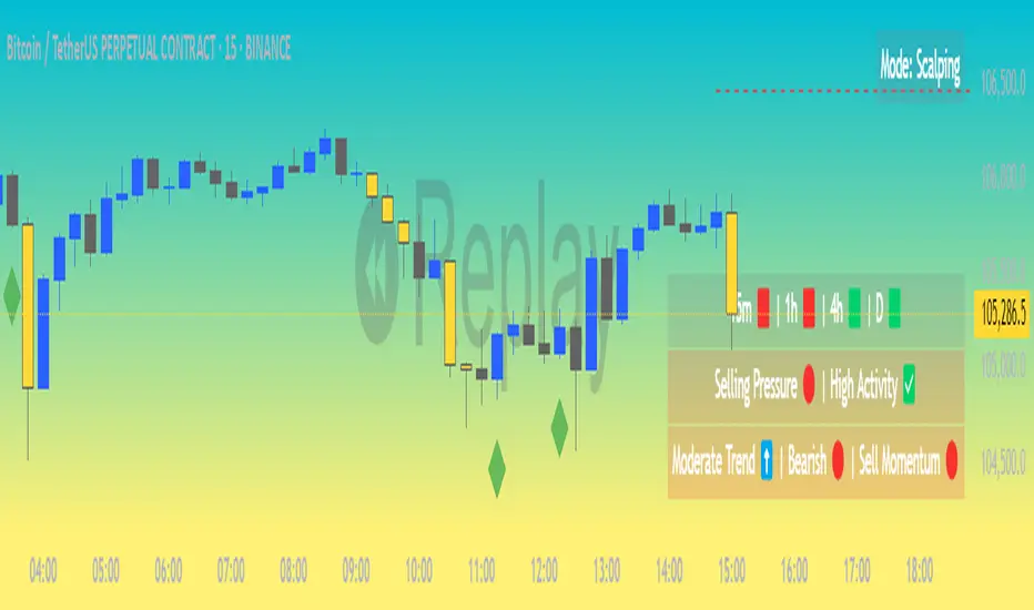
Market Matrix ViewThis technical indicator is designed to provide traders with a quick and integrated view of market dynamics by combining several popular indicators into a single tool. It's not a magic bullet, but a practical aid for analyzing buying/selling pressure, trends, volume, and divergences, saving you time in the decision-making process. Built for flexibility, the indicator adapts to various trading styles (scalping, swing, or long-term) and offers customizable settings to suit your needs.
🟡 Multi-Timeframe Trends
➤ This section displays the trend direction (bullish, bearish, or neutral) across 15-minute, 1-hour, 4-hour, and Daily timeframes, providing multi-timeframe market context. Timeframes lower than the one currently selected will show "N/A."
➤It utilizes fast and slow Exponential Moving Averages (EMAs) for each timeframe:
15m: Fast EMA 42, Slow EMA 170
1h: Fast EMA 40, Slow EMA 100
4h: Fast EMA 36, Slow EMA 107
Daily: Fast EMA 20, Slow EMA 60
🟡 Smart Flow & RVOL
➤ This section displays "Buying Pressure" or "Selling Pressure" signals based on indicator confluence, alongside volume activity ("High Activity," "Normal Activity," or "Low Activity").
➤ Smart Flow combines Chaikin Money Flow (CMF) and Money Flow Index (MFI) to detect buying/selling pressure. CMF measures money flow based on price position within the high-low range, while MFI analyzes money flow considering typical price and volume. A signal is generated only when both indicators simultaneously increase/decrease beyond an adjustable threshold ("Buy/Sell Sensitivity") and volume exceeds a Simple Moving Average (SMA) scaled by the "Volume Multiplier."
➤ RVOL (Relative Volume) calculates relative volume separately for bullish and bearish candles, comparing recent volume (fast SMA) with a reference volume (slow SMA). Thresholds are adjusted based on the selected mode.
🟡 ADX & RSI
This section displays trend strength ("Strong," "Moderate," or "Weak"), its direction ("Bullish" or "Bearish"), and the RSI momentum status ("Overbought," "Oversold," "Buy/Sell Momentum," or "Neutral").
➤ ADX (Average Directional Index) measures trend strength (above 40 = "Strong," 20–40 = "Moderate," below 20 = "Weak"). Direction is determined by comparing +DI (upward movement) with -DI (downward movement). Additionally, an arrow indicates whether the trend's strength is decreasing or increasing.
➤RSI (Relative Strength Index) evaluates price momentum. Extreme levels (above 80/85 = "Overbought," below 15/20 = "Oversold") and intermediate zones (47–53 = "Neutral," above 53 = "Buy Momentum," below 47 = "Sell Momentum") are adjusted based on the selected mode.
🟡 When these signals are active for a potential trade setup, the table's background lights up green or red, respectively.
🟡 Volume Spikes
➤This feature highlights bars with significantly higher volume than the recent average, coloring them yellow on the chart to draw attention to intense market activity.
➤It uses the Z-Score method to detect volume anomalies. Current volume is compared to a 10-bar Simple Moving Average (SMA) and the standard deviation of volume over the same period. If the Z-Score exceeds a certain threshold, the bar is marked as a volume spike.
🟡 Divergences (Volume Divergence Detection)
➤ This feature marks divergences between price and technical indicators on the chart, using diamond-shaped labels (green for bullish divergences, red for bearish divergences) to signal potential trend reversals.
➤ It compares price deviations from a Simple Moving Average (SMA) with deviations of three indicators: Chaikin Money Flow (CMF), Money Flow Index (MFI), and On-Balance Volume (OBV). A bullish divergence occurs when price falls below its average, but CMF, MFI, and OBV rise above their averages, indicating hidden accumulation. A bearish divergence occurs when price rises above its average, but CMF, MFI, and OBV fall, suggesting distribution. The length of the moving averages is adjustable (default 13/10/5 bars for Scalping/Balanced/Swing), and detection thresholds are scaled by "Divergence Sensitivity" (default 1.0).
🟡 Adaptive Stop-Loss (ATR)
➤Draws dynamic stop-loss lines (red, dashed) on the chart for buy or sell signals, helping traders manage risk.Uses the Average True Range (ATR) to calculate stop-loss levels, set at low/high ± ATR × multiplier
🟡 Alerts for trend direction changes in the Info Panel:
➤ Triggers notifications when the trend shifts to Bullish (when +DI crosses above -DI) or Bearish (when +DI crosses below -DI), helping you stay informed about key market shifts.
How to use: Set alerts in Trading View for “Trend Changed to Bullish” or “Trend Changed to Bearish” with “Once Per Bar Close” for reliable signals.
🟡 Settings (Inputs)
➤ The indicator offers customizable settings to fit your trading style, but it's already optimized for Scalping (1m–15m), Balanced (16m–3h59m), and Swing (4h–Daily) modes, which automatically adjust based on the selected timeframe. The visible inputs allow you to adjust the following parameters:
Show Info Panel: Enables/disables the information panel (default: enabled).
Show Volume Spikes: Turns on/off coloring for volume spike bars (default: enabled).
Spike Sensitivity: Controls the Z-Score threshold for detecting volume spikes (default: 2.0; lower values increase signal frequency).
Show Divergence: Enables/disables the display of divergence labels (default: enabled).
Divergence Sensitivity: Adjusts the thresholds for divergence detection (default: 1.0; higher values reduce sensitivity).
Divergence Lookback Length: Sets the length of the moving averages used for divergences (default: 5, automatically adjusted to 13/10/5 for Scalping/Balanced/Swing).
RVOL Reference Period: Defines the reference period for relative volume (default: 20, automatically adjusted to 7/15/20).
RSI Length: Sets the RSI length (default: 14, automatically adjusted to 5/10/14).
Buy Sensitivity: Controls the increase threshold for Buying Pressure signals (default: 0.007; higher values reduce frequency).
Sell Sensitivity: Controls the decrease threshold for Selling Pressure signals (default: 0.007; higher values reduce frequency).
Volume Multiplier (B/S Pressure): Adjusts the volume threshold for Smart Flow signals (default: 0.6; higher values require greater volume).
🟡 This indicator is created to simplify market analysis, but I am not a professional in Pine Script or technical indicators. This indicator is not a standalone solution. For optimal results, it must be integrated into a well-defined trading strategy that includes risk management and other confirmations.
SPX Weekly Expected Moves# SPX Weekly Expected Moves Indicator
A professional Pine Script indicator for TradingView that displays weekly expected move levels for SPX based on real options data, with integrated Fibonacci retracement analysis and intelligent alerting system.
## Overview
This indicator helps options and equity traders visualize weekly expected move ranges for the S&P 500 Index (SPX) by plotting historical and current week expected move boundaries derived from weekly options pricing. Unlike theoretical volatility calculations, this indicator uses actual market-based expected move data that you provide from options platforms.
## Key Features
### 📈 **Expected Move Visualization**
- **Historical Lines**: Display past weeks' expected moves with configurable history (10, 26, or 52 weeks)
- **Current Week Focus**: Highlighted current week with extended lines to present time
- **Friday Close Reference**: Orange baseline showing the previous Friday's close price
- **Timeframe Independent**: Works consistently across all chart timeframes (1m to 1D)
### 🎯 **Fibonacci Integration**
- **Five Fibonacci Levels**: 23.6%, 38.2%, 50%, 61.8%, 76.4% between Friday close and expected move boundaries
- **Color-Coded Levels**:
- Red: 23.6% & 76.4% (outer levels)
- Blue: 38.2% & 61.8% (golden ratio levels)
- Black: 50% (midpoint - most critical level)
- **Current Week Only**: Fibonacci levels shown only for active trading week to reduce clutter
### 📊 **Real-Time Information Table**
- **Current SPX Price**: Live market price
- **Expected Move**: ±EM value for current week
- **Previous Close**: Friday close price (baseline for calculations)
- **100% EM Levels**: Exact upper and lower boundary prices
- **Current Location**: Real-time position within the EM structure (e.g., "Above 38.2% Fib (upper zone)")
### 🚨 **Intelligent Alert System**
- **Zone-Aware Alerts**: Separate alerts for upper and lower zones
- **Key Level Breaches**: Alerts for 23.6% and 76.4% Fibonacci level crossings
- **Bar Close Based**: Alerts trigger on confirmed bar closes, not tick-by-tick
- **Customizable**: Enable/disable alerts through settings
## How It Works
### Data Input Method
The indicator uses a **manual data entry approach** where you input actual expected move values obtained from options platforms:
```pinescript
// Add entries using the options expiration Friday date
map.put(expected_moves, 20250613, 91.244) // Week ending June 13, 2025
map.put(expected_moves, 20250620, 95.150) // Week ending June 20, 2025
```
### Weekly Structure
- **Monday 9:30 AM ET**: Week begins
- **Friday 4:00 PM ET**: Week ends
- **Lines Extend**: From Monday open to Friday close (historical) or current time + 5 bars (current week)
- **Timezone Handling**: Uses "America/New_York" for proper DST handling
### Calculation Logic
1. **Base Price**: Previous Friday's SPX close price
2. **Expected Move**: Market-derived ±EM value from weekly options
3. **Upper Boundary**: Friday Close + Expected Move
4. **Lower Boundary**: Friday Close - Expected Move
5. **Fibonacci Levels**: Proportional levels between Friday close and EM boundaries
## Setup Instructions
### 1. Data Collection
Obtain weekly expected move values from options platforms such as:
- **ThinkOrSwim**: Use thinkBack feature to look up weekly expected moves
- **Tastyworks**: Check weekly options expected move data
- **CBOE**: Reference SPX weekly options data
- **Manual Calculation**: (ATM Call Premium + ATM Put Premium) × 0.85
### 2. Data Entry
After each Friday close, update the indicator with the next week's expected move:
```pinescript
// Example: On Friday June 7, 2025, add data for week ending June 13
map.put(expected_moves, 20250613, 91.244) // Actual EM value from your platform
```
### 3. Configuration
Customize the indicator through the settings panel:
#### Visual Settings
- **Show Current Week EM**: Toggle current week display
- **Show Past Weeks**: Toggle historical weeks display
- **Max Weeks History**: Choose 10, 26, or 52 weeks of history
- **Show Fibonacci Levels**: Toggle Fibonacci retracement levels
- **Label Controls**: Customize which labels to display
#### Colors
- **Current Week EM**: Default yellow for active week
- **Past Weeks EM**: Default gray for historical weeks
- **Friday Close**: Default orange for baseline
- **Fibonacci Levels**: Customizable colors for each level type
#### Alerts
- **Enable EM Breach Alerts**: Master toggle for all alerts
- **Specific Alerts**: Four alert types for Fibonacci level breaches
## Trading Applications
### Options Trading
- **Straddle/Strangle Positioning**: Visualize breakeven levels for neutral strategies
- **Directional Plays**: Assess probability of reaching target levels
- **Earnings Plays**: Compare actual vs. expected move outcomes
### Equity Trading
- **Support/Resistance**: Use EM boundaries and Fibonacci levels as key levels
- **Breakout Trading**: Monitor for moves beyond expected ranges
- **Mean Reversion**: Look for reversals at extreme Fibonacci levels
### Risk Management
- **Position Sizing**: Gauge likely price ranges for the week
- **Stop Placement**: Use Fibonacci levels for logical stop locations
- **Profit Targets**: Set targets based on EM structure probabilities
## Technical Implementation
### Performance Features
- **Memory Managed**: Configurable history limits prevent memory issues
- **Timeframe Independent**: Uses timestamp-based calculations for consistency
- **Object Management**: Automatic cleanup of drawing objects prevents duplicates
- **Error Handling**: Robust bounds checking and NA value handling
### Pine Script Best Practices
- **v6 Compliance**: Uses latest Pine Script version features
- **User Defined Types**: Structured data management with WeeklyEM type
- **Efficient Drawing**: Smart line/label creation and deletion
- **Professional Standards**: Clean code organization and comprehensive documentation
## Customization Guide
### Adding New Weeks
```pinescript
// Add after market close each Friday
map.put(expected_moves, YYYYMMDD, EM_VALUE)
```
### Color Schemes
Customize colors for different trading styles:
- **Dark Theme**: Use bright colors for visibility
- **Light Theme**: Use contrasting dark colors
- **Minimalist**: Use single color with transparency
### Label Management
Control label density:
- **Show Current Week Labels Only**: Reduce clutter for active trading
- **Show All Labels**: Full information for analysis
- **Selective Display**: Choose specific label types
## Troubleshooting
### Common Issues
1. **No Lines Appearing**: Check that expected move data is entered for current/recent weeks
2. **Wrong Time Display**: Ensure "America/New_York" timezone is properly handled
3. **Duplicate Lines**: Restart indicator if drawing objects appear duplicated
4. **Missing Fibonacci Levels**: Verify "Show Fibonacci Levels" is enabled
### Data Validation
- **Expected Move Format**: Use positive numbers (e.g., 91.244, not ±91.244)
- **Date Format**: Use YYYYMMDD format (e.g., 20250613)
- **Reasonable Values**: Verify EM values are realistic (typically 50-200 for SPX)
## Version History
### Current Version
- **Pine Script v6**: Latest version compatibility
- **Fibonacci Integration**: Five-level retracement analysis
- **Zone-Aware Alerts**: Upper/lower zone differentiation
- **Dynamic Line Management**: Smart current week extension
- **Professional UI**: Comprehensive information table
### Future Enhancements
- **Multiple Symbols**: Extend beyond SPX to other indices
- **Automated Data**: Integration with options data APIs
- **Statistical Analysis**: Success rate tracking for EM predictions
- **Additional Levels**: Custom percentage levels beyond Fibonacci
## License & Usage
This indicator is designed for educational and trading purposes. Users are responsible for:
- **Data Accuracy**: Ensuring correct expected move values
- **Risk Management**: Proper position sizing and risk controls
- **Market Understanding**: Comprehending options-based expected move concepts
## Support
For questions, issues, or feature requests related to this indicator, please refer to the code comments and documentation within the Pine Script file.
---
**Disclaimer**: This indicator is for informational purposes only. Trading involves substantial risk of loss and is not suitable for all investors. Past performance does not guarantee future results.

NY ORB + Fakeout Detector🗽 NY ORB + Fakeout Detector
This indicator automatically plots the New York Opening Range (ORB) based on the first 15 minutes of the NY session (15:30–15:45 CEST / 13:30–13:45 UTC) and detects potential fakeouts (false breakouts).
🔍 Key Features:
✅ Plots ORB high and low based on the 15-minute NY open range
✅ Automatically detects fake breakouts (price wicks beyond the box but closes back inside)
✅ Visual markers:
🔺 "Fake ↑" if a fake breakout occurs above the range
🔻 "Fake ↓" if a fake breakout occurs below the range
✅ Gray background highlights the ORB session window
✅ Designed for scalping and short-term breakout strategies
🧠 Best For:
Intraday traders looking for NY volatility setups
Scalpers using ORB-based entries
Traders seeking early-session fakeout traps to avoid false signals
Those combining with EMA 12/21, volume, or other confluence tools

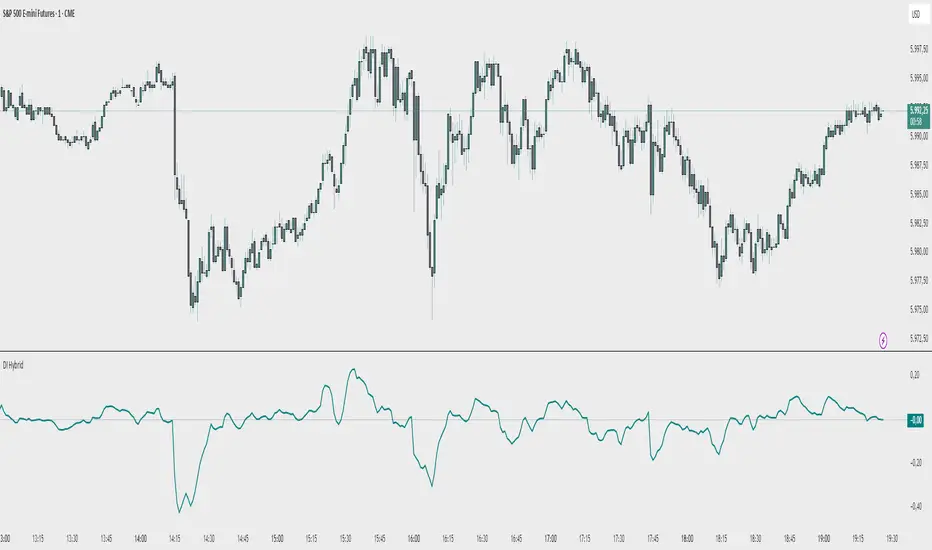
Demand Index (Hybrid Sibbet) by TradeQUODemand Index (Hybrid Sibbet) by TradeQUO \
\Overview\
The Demand Index (DI) was introduced by James Sibbet in the early 1990s to gauge “real” buying versus selling pressure by combining price‐change information with volume intensity. Unlike pure price‐based oscillators (e.g. RSI or MACD), the DI highlights moves backed by above‐average volume—helping traders distinguish genuine demand/supply from false breakouts or low‐liquidity noise.
\Calculation\
\
\ \Step 1: Weighted Price (P)\
For each bar t, compute a weighted price:
```
Pₜ = Hₜ + Lₜ + 2·Cₜ
```
where Hₜ=High, Lₜ=Low, Cₜ=Close of bar t.
Also compute Pₜ₋₁ for the prior bar.
\ \Step 2: Raw Range (R)\
Calculate the two‐bar range:
```
Rₜ = max(Hₜ, Hₜ₋₁) – min(Lₜ, Lₜ₋₁)
```
This Rₜ is used indirectly in the exponential dampener below.
\ \Step 3: Normalize Volume (VolNorm)\
Compute an EMA of volume over n₁ bars (e.g. n₁=13):
```
EMA_Volₜ = EMA(Volume, n₁)ₜ
```
Then
```
VolNormₜ = Volumeₜ / EMA_Volₜ
```
If EMA\_Volₜ ≈ 0, set VolNormₜ to a small default (e.g. 0.0001) to avoid division‐by‐zero.
\ \Step 4: BuyPower vs. SellPower\
Calculate “raw” BuyPowerₜ and SellPowerₜ depending on whether Pₜ > Pₜ₋₁ (bullish) or Pₜ < Pₜ₋₁ (bearish). Use an exponential dampener factor Dₜ to moderate extreme moves when true range is small. Specifically:
• If Pₜ > Pₜ₋₁,
```
BuyPowerₜ = (VolNormₜ) / exp
```
otherwise
```
BuyPowerₜ = VolNormₜ.
```
• If Pₜ < Pₜ₋₁,
```
SellPowerₜ = (VolNormₜ) / exp
```
otherwise
```
SellPowerₜ = VolNormₜ.
```
Here, H₀ and L₀ are the very first bar’s High/Low—used to calibrate the scale of the dampening. If the denominator of the exponential is near zero, substitute a small epsilon (e.g. 1e-10).
\ \Step 5: Smooth Buy/Sell Power\
Apply a short EMA (n₂ bars, typically n₂=2) to each:
```
EMA_Buyₜ = EMA(BuyPower, n₂)ₜ
EMA_Sellₜ = EMA(SellPower, n₂)ₜ
```
\ \Step 6: Raw Demand Index (DI\_raw)\
```
DI_rawₜ = EMA_Buyₜ – EMA_Sellₜ
```
A positive DI\_raw indicates that buying force (normalized by volume) exceeds selling force; a negative value indicates the opposite.
\ \Step 7: Optional EMA Smoothing on DI (DI)\
To reduce choppiness, compute an EMA over DI\_raw (n₃ bars, e.g. n₃ = 1–5):
```
DIₜ = EMA(DI_raw, n₃)ₜ.
```
If n₃ = 1, DI = DI\_raw (no further smoothing).
\
\Interpretation\
\
\ \Crossing Zero Line\
• DI\_raw (or DI) crossing from below to above zero signals that cumulative buying pressure (over the chosen smoothing window) has overcome selling pressure—potential Long signal.
• Crossing from above to below zero signals dominant selling pressure—potential Short signal.
\ \DI\_raw vs. DI (EMA)\
• When DI\_raw > DI (the EMA of DI\_raw), bullish momentum is accelerating.
• When DI\_raw < DI, bullish momentum is weakening (or bearish acceleration).
\ \Divergences\
• If price makes new highs while DI fails to make higher highs (DI\_raw or DI declining), this hints at weakening buying power (“bearish divergence”), possibly preceding a reversal.
• If price makes new lows while DI fails to make lower lows (“bullish divergence”), this may signal waning selling pressure and a potential bounce.
\ \Volume Confirmation\
• A strong price move without a corresponding rise in DI often indicates low‐volume “fake” moves.
• Conversely, a modest price move with a large DI spike suggests true institutional participation—often a more reliable breakout.
\
\Usage Notes & Warnings\
\
\ \Never Use DI in Isolation\
It is a \filter\ and \confirmation\ tool—combine with price‐action (trendlines, support/resistance, candlestick patterns) and risk management (stop‐losses) before executing trades.
\ \Parameter Selection\
• \Vol EMA length (n₁)\: Commonly 13–20 bars. Shorter → more responsive to volume spikes, but noisier.
• \Buy/Sell EMA length (n₂)\: Typically 2 bars for fast smoothing.
• \DI smoothing (n₃)\: Usually 1 (no smoothing) or 3–5 for moderate smoothing. Long DI\_EMA (e.g. 20–50) gives a slower signal.
\ \Market Adaptation\
Works well in liquid futures, indices, and heavily traded stocks. In thinly traded or highly erratic markets, adjust n₁ upward (e.g., 20–30) to reduce noise.
---
\In Summary\
The Demand Index (James Sibbet) uses a three‐stage smoothing (volume → Buy/Sell Power → DI) to reveal true demand/supply imbalance. By combining normalized volume with price change, Sibbet’s DI helps traders identify momentum backed by real participation—filtering out “empty” moves and spotting early divergences. Always confirm DI signals with price action and sound risk controls before trading.
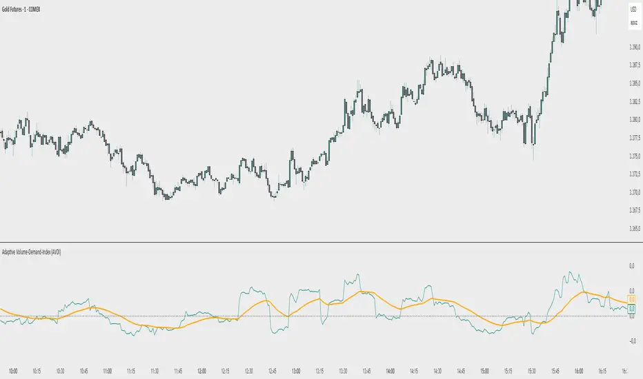
Adaptive Volume‐Demand‐Index (AVDI)Demand Index (according to James Sibbet) – Short Description
The Demand Index (DI) was developed by James Sibbet to measure real “buying” vs. “selling” strength (Demand vs. Supply) using price and volume data. It is not a standalone trading signal, but rather a filter and trend confirmer that should always be used together with chart structure and additional indicators.
---
\ 1. Calculation Basis\
1. Volume Normalization
$$
\text{normVol}_t
= \frac{\text{Volume}_t}{\mathrm{EMA}(\text{Volume},\,n_{\text{Vol}})_t}
\quad(\text{e.g., }n_{\text{Vol}} = 13)
$$
This smooths out extremely high volume spikes and compares them to the average (≈ 1 means “average volume”).
2. Price Factor
$$
\text{priceFactor}_t
= \frac{\text{Close}_t - \text{Open}_t}{\text{Open}_t}.
$$
Positive values for bullish bars, negative for bearish bars.
3. Component per Bar
$$
\text{component}_t
= \text{normVol}_t \times \text{priceFactor}_t.
$$
If volume is above average (> 1) and the price rises slightly, this yields a noticeably positive value; conversely if the price falls.
4. Raw DI (Rolling Sum)
Over a window of \$w\$ bars (e.g., 20):
$$
\text{RawDI}_t
= \sum_{i=0}^{w-1} \text{component}_{\,t-i}.
$$
Alternatively, recursively for \$t \ge w\$:
$$
\text{RawDI}_t
= \text{RawDI}_{t-1}
+ \text{component}_t
- \text{component}_{\,t-w}.
$$
5. Optional EMA Smoothing
An EMA over RawDI (e.g., \$n\_{\text{DI}} = 50\$) reduces short-term fluctuations and highlights medium-term trends:
$$
\text{EMA\_DI}_t
= \mathrm{EMA}(\text{RawDI},\,n_{\text{DI}})_t.
$$
6.Zero Line
Handy guideline:
RawDI > 0: Accumulated buying power dominates.
RawDI < 0: Accumulated selling power dominates.
2. Interpretation & Application
Crossing Zero
RawDI above zero → Indication of increasing buying pressure (potential long signal).
RawDI below zero → Indication of increasing selling pressure (potential short signal).
Not to be used alone for entry—always confirm with price action.
RawDI vs. EMA_DI
RawDI > EMA\_DI → Acceleration of demand.
RawDI < EMA\_DI → Weakening of demand.
Divergences
Price makes a new high, RawDI does not make a higher high → potential weakness in the uptrend.
Price makes a new low, RawDI does not make a lower low → potential exhaustion of the downtrend.
3. Typical Signals (for Beginners)
\ 1. Long Setup\
RawDI crosses zero from below,
RawDI > EMA\_DI (acceleration),
Price closes above a short-term swing high or resistance.
Stop-Loss: just below the last swing low, Take-Profit/Trailing: on reversal signals or fixed R\:R.
2. Short Setup
RawDI crosses zero from above,
RawDI < EMA\_DI (increased selling pressure),
Price closes below a short-term swing low or support.
Stop-Loss: just above the last swing high.
---
4. Notes and Parameters
Recommended Values (Beginners):
Volume EMA (n₍Vol₎) = 13
RawDI window (w) = 20
EMA over DI (n₍DI₎) = 50 (medium-term) or 1 (no smoothing)
Attention:\
NEVER use in isolation. Always in combination with price action analysis (trendlines, support/resistance, candlestick patterns).
Especially during volatile news phases, RawDI can fluctuate strongly → EMA\_DI helps to avoid false signals.
---
Conclusion The Demand Index by James Sibbet is a powerful filter to assess price movements by their volume backing. It shows whether a rally is truly driven by demand or merely a short-term volume anomaly. In combination with classic chart analysis and risk management, it helps to identify robust entry points and potential trend reversals earlier.
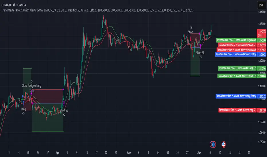
TrendMaster Pro 2.3 with Alerts
Hello friends,
A member of the community approached me and asked me how to write an indicator that would achieve a particular set of goals involving comprehensive trend analysis, risk management, and session-based trading controls. Here is one example method of how to create such a system:
Core Strategy Components
Multi-Moving Average System - Uses configurable MA types (EMA, SMA, SMMA) with short-term (9) and long-term (21) periods for primary signal generation through crossovers
Higher Timeframe Trend Filter - Optional trend confirmation using a separate MA (default 50-period) to ensure trades align with broader market direction
Band Power Indicator - Dynamic high/low bands calculated using different MA types to identify price channels and volatility zones
Advanced Signal Filtering
Bollinger Bands Volatility Filter - Prevents trading during low-volatility ranging markets by requiring sufficient band width
RSI Momentum Filter - Uses customizable thresholds (55 for longs, 45 for shorts) to confirm momentum direction
MACD Trend Confirmation - Ensures MACD line position relative to signal line aligns with trade direction
Stochastic Oscillator - Adds momentum confirmation with overbought/oversold levels
ADX Strength Filter - Only allows trades when trend strength exceeds 25 threshold
Session-Based Trading Management
Four Trading Sessions - Asia (18:00-00:00), London (00:00-08:00), NY AM (08:00-13:00), NY PM (13:00-18:00)
Individual Session Limits - Separate maximum trade counts for each session (default 5 per session)
Automatic Session Closure - All positions close at specified market close time
Risk Management Features
Multiple Stop Loss Options - Percentage-based, MA cross, or band-based SL methods
Risk/Reward Ratio - Configurable TP levels based on SL distance (default 1:2)
Auto-Risk Calculation - Dynamic position sizing based on dollar risk limits ($150-$250 range)
Daily Limits - Stop trading after reaching specified TP or SL counts per day
Support & Resistance System
Multiple Pivot Types - Traditional, Fibonacci, Woodie, Classic, DM, and Camarilla calculations
Flexible Timeframes - Auto-adjusting or manual timeframe selection for S/R levels
Historical Levels - Configurable number of past S/R levels to display
Visual Customization - Individual color and display settings for each S/R level
Additional Features
Alert System - Customizable buy/sell alert messages with once-per-bar frequency
Visual Trade Management - Color-coded entry, SL, and TP levels with fill areas
Session Highlighting - Optional background colors for different trading sessions
Comprehensive Filtering - All signals must pass through multiple confirmation layers before execution
This approach demonstrates how to build a professional-grade trading system that combines multiple technical analysis methods with robust risk management and session-based controls, suitable for algorithmic trading across different market sessions.
Good luck and stay safe!
DECODE Global Liquidity IndexDECODE Global Liquidity Index 🌊
The DECODE Global Liquidity Index is a powerful tool designed to track and aggregate global liquidity by combining data from the world's 13 largest economies. It offers a comprehensive view of financial liquidity, providing crucial insights into the underlying currents that can influence asset prices and market trends.
The economies covered are: United States, China, European Union, Japan, India, United Kingdom, Brazil, Canada, Russia, South Korea, Australia, Mexico, and Indonesia. The European Union accounts for major individual economies within the EU like Germany, France, Italy, Spain, Netherlands, Poland, etc.
Key Features:
1. Customizable Liquidity Sources
Include Global M2: You can opt to include the M2 money supply from the 13 listed economies. M2 is a broad measure of money supply that includes cash, checking deposits, savings deposits, money market securities, mutual funds, and other time deposits. (Note: Australia uses M3 as its primary measure, which is included when M2 is selected for Australia).
Include Central Bank Balance Sheets (CBBS): Alternatively, or in addition, you can include the total assets held by the central banks of these economies. Central bank balance sheets expand or contract based on monetary policy operations like quantitative easing (QE) or tightening (QT).
Combined View: If you select both M2 and CBBS, and data is available for both, the indicator will display an average of the two aggregated values. If only one source type is selected, or if data for one type is unavailable despite both being selected, the indicator will display the single available and selected component. This provides flexibility in how you define and analyze global liquidity.
2. Lead/Lag Analysis (Forward Projection):
Lead Offset (Days): This feature allows you to project the liquidity index forward by a specified number of days.
Why it's useful: Global liquidity changes can often be a leading indicator for various asset classes, particularly those sensitive to risk appetite, like Bitcoin or growth stocks. These assets might lag shifts in liquidity. By applying a lead (e.g., 90 days), you can shift the liquidity data forward on your chart to more easily visualize potential correlations and identify if current asset price movements might be responding to past changes in liquidity.
3. Rate of Change (RoC) Oscillator:
Year-over-Year % View: Instead of viewing aggregate liquidity, you can switch to a Year-over-Year (YoY%) Rate of Change (ROC) oscillator.
Why it's useful:
Momentum Identification: The ROC highlights the speed and direction of liquidity changes. Positive values indicate liquidity is increasing compared to a year ago, while negative values show it's decreasing.
Turning Points: Oscillators make it easier to spot potential accelerations, decelerations, or reversals in liquidity trends. A cross above the zero line can signal strengthening liquidity momentum, while a cross below can signal weakening momentum.
Cycle Analysis: It helps in assessing the cyclical nature of liquidity provision and its potential impact on market cycles.
This indicator aims to provide a clear, customizable, and insightful measure of global liquidity to aid traders and investors in their market analysis.
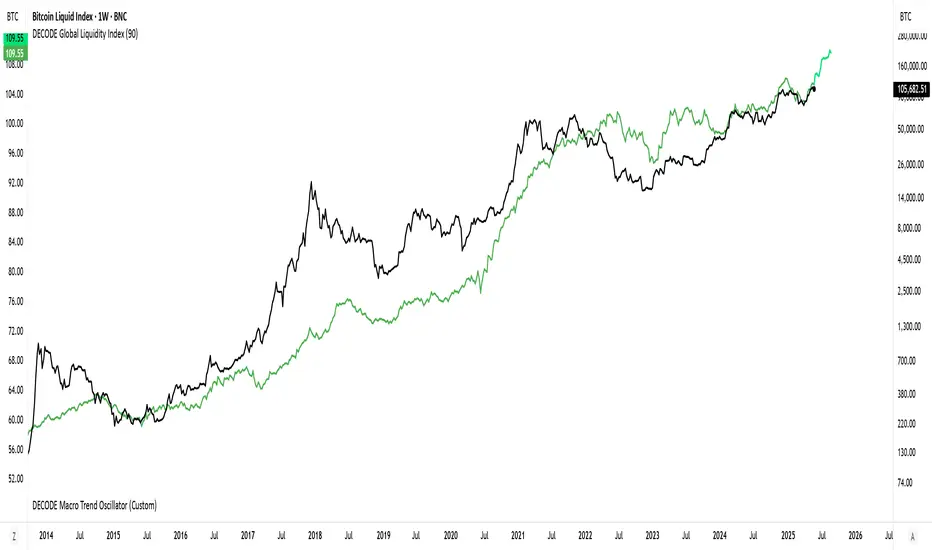
Advanced Petroleum Market Model (APMM)Advanced Petroleum Market Model (APMM): A Multi-Factor Fundamental Analysis Framework for Oil Market Assessment
## 1. Introduction
The petroleum market represents one of the most complex and globally significant commodity markets, characterized by intricate supply-demand dynamics, geopolitical influences, and substantial price volatility (Hamilton, 2009). Traditional fundamental analysis approaches often struggle to synthesize the multitude of relevant indicators into actionable insights due to data heterogeneity, temporal misalignment, and subjective weighting schemes (Baumeister & Kilian, 2016).
The Advanced Petroleum Market Model addresses these limitations through a systematic, quantitative approach that integrates 16 verified fundamental indicators across five critical market dimensions. The model builds upon established financial engineering principles while incorporating petroleum-specific market dynamics and adaptive learning mechanisms.
## 2. Theoretical Framework
### 2.1 Market Efficiency and Information Integration
The model operates under the assumption of semi-strong market efficiency, where fundamental information is gradually incorporated into prices with varying degrees of lag (Fama, 1970). The petroleum market's unique characteristics, including storage costs, transportation constraints, and geopolitical risk premiums, create opportunities for fundamental analysis to provide predictive value (Kilian, 2009).
### 2.2 Multi-Factor Asset Pricing Theory
Drawing from Ross's (1976) Arbitrage Pricing Theory, the model treats petroleum prices as driven by multiple systematic risk factors. The five-factor decomposition (Supply, Inventory, Demand, Trade, Sentiment) represents economically meaningful sources of systematic risk in petroleum markets (Chen et al., 1986).
## 3. Methodology
### 3.1 Data Sources and Quality Framework
The model integrates 16 fundamental indicators sourced from verified TradingView economic data feeds:
Supply Indicators:
- US Oil Production (ECONOMICS:USCOP)
- US Oil Rigs Count (ECONOMICS:USCOR)
- API Crude Runs (ECONOMICS:USACR)
Inventory Indicators:
- US Crude Stock Changes (ECONOMICS:USCOSC)
- Cushing Stocks (ECONOMICS:USCCOS)
- API Crude Stocks (ECONOMICS:USCSC)
- API Gasoline Stocks (ECONOMICS:USGS)
- API Distillate Stocks (ECONOMICS:USDS)
Demand Indicators:
- Refinery Crude Runs (ECONOMICS:USRCR)
- Gasoline Production (ECONOMICS:USGPRO)
- Distillate Production (ECONOMICS:USDFP)
- Industrial Production Index (FRED:INDPRO)
Trade Indicators:
- US Crude Imports (ECONOMICS:USCOI)
- US Oil Exports (ECONOMICS:USOE)
- API Crude Imports (ECONOMICS:USCI)
- Dollar Index (TVC:DXY)
Sentiment Indicators:
- Oil Volatility Index (CBOE:OVX)
### 3.2 Data Quality Monitoring System
Following best practices in quantitative finance (Lopez de Prado, 2018), the model implements comprehensive data quality monitoring:
Data Quality Score = Σ(Individual Indicator Validity) / Total Indicators
Where validity is determined by:
- Non-null data availability
- Positive value validation
- Temporal consistency checks
### 3.3 Statistical Normalization Framework
#### 3.3.1 Z-Score Normalization
The model employs robust Z-score normalization as established by Sharpe (1994) for cross-indicator comparability:
Z_i,t = (X_i,t - μ_i) / σ_i
Where:
- X_i,t = Raw value of indicator i at time t
- μ_i = Sample mean of indicator i
- σ_i = Sample standard deviation of indicator i
Z-scores are capped at ±3 to mitigate outlier influence (Tukey, 1977).
#### 3.3.2 Percentile Rank Transformation
For intuitive interpretation, Z-scores are converted to percentile ranks following the methodology of Conover (1999):
Percentile_Rank = (Number of values < current_value) / Total_observations × 100
### 3.4 Exponential Smoothing Framework
Signal smoothing employs exponential weighted moving averages (Brown, 1963) with adaptive alpha parameter:
S_t = α × X_t + (1-α) × S_{t-1}
Where α = 2/(N+1) and N represents the smoothing period.
### 3.5 Dynamic Threshold Optimization
The model implements adaptive thresholds using Bollinger Band methodology (Bollinger, 1992):
Dynamic_Threshold = μ ± (k × σ)
Where k is the threshold multiplier adjusted for market volatility regime.
### 3.6 Composite Score Calculation
The fundamental score integrates component scores through weighted averaging:
Fundamental_Score = Σ(w_i × Score_i × Quality_i)
Where:
- w_i = Normalized component weight
- Score_i = Component fundamental score
- Quality_i = Data quality adjustment factor
## 4. Implementation Architecture
### 4.1 Adaptive Parameter Framework
The model incorporates regime-specific adjustments based on market volatility:
Volatility_Regime = σ_price / μ_price × 100
High volatility regimes (>25%) trigger enhanced weighting for inventory and sentiment components, reflecting increased market sensitivity to supply disruptions and psychological factors.
### 4.2 Data Synchronization Protocol
Given varying publication frequencies (daily, weekly, monthly), the model employs forward-fill synchronization to maintain temporal alignment across all indicators.
### 4.3 Quality-Adjusted Scoring
Component scores are adjusted for data quality to prevent degraded inputs from contaminating the composite signal:
Adjusted_Score = Raw_Score × Quality_Factor + 50 × (1 - Quality_Factor)
This formulation ensures that poor-quality data reverts toward neutral (50) rather than contributing noise.
## 5. Usage Guidelines and Best Practices
### 5.1 Configuration Recommendations
For Short-term Analysis (1-4 weeks):
- Lookback Period: 26 weeks
- Smoothing Length: 3-5 periods
- Confidence Period: 13 weeks
- Increase inventory and sentiment weights
For Medium-term Analysis (1-3 months):
- Lookback Period: 52 weeks
- Smoothing Length: 5-8 periods
- Confidence Period: 26 weeks
- Balanced component weights
For Long-term Analysis (3+ months):
- Lookback Period: 104 weeks
- Smoothing Length: 8-12 periods
- Confidence Period: 52 weeks
- Increase supply and demand weights
### 5.2 Signal Interpretation Framework
Bullish Signals (Score > 70):
- Fundamental conditions favor price appreciation
- Consider long positions or reduced short exposure
- Monitor for trend confirmation across multiple timeframes
Bearish Signals (Score < 30):
- Fundamental conditions suggest price weakness
- Consider short positions or reduced long exposure
- Evaluate downside protection strategies
Neutral Range (30-70):
- Mixed fundamental environment
- Favor range-bound or volatility strategies
- Wait for clearer directional signals
### 5.3 Risk Management Considerations
1. Data Quality Monitoring: Continuously monitor the data quality dashboard. Scores below 75% warrant increased caution.
2. Regime Awareness: Adjust position sizing based on volatility regime indicators. High volatility periods require reduced exposure.
3. Correlation Analysis: Monitor correlation with crude oil prices to validate model effectiveness.
4. Fundamental-Technical Divergence: Pay attention when fundamental signals diverge from technical indicators, as this may signal regime changes.
### 5.4 Alert System Optimization
Configure alerts conservatively to avoid false signals:
- Set alert threshold at 75+ for high-confidence signals
- Enable data quality warnings to maintain system integrity
- Use trend reversal alerts for early regime change detection
## 6. Model Validation and Performance Metrics
### 6.1 Statistical Validation
The model's statistical robustness is ensured through:
- Out-of-sample testing protocols
- Rolling window validation
- Bootstrap confidence intervals
- Regime-specific performance analysis
### 6.2 Economic Validation
Fundamental accuracy is validated against:
- Energy Information Administration (EIA) official reports
- International Energy Agency (IEA) market assessments
- Commercial inventory data verification
## 7. Limitations and Considerations
### 7.1 Model Limitations
1. Data Dependency: Model performance is contingent on data availability and quality from external sources.
2. US Market Focus: Primary data sources are US-centric, potentially limiting global applicability.
3. Lag Effects: Some fundamental indicators exhibit publication lags that may delay signal generation.
4. Regime Shifts: Structural market changes may require model recalibration.
### 7.2 Market Environment Considerations
The model is optimized for normal market conditions. During extreme events (e.g., geopolitical crises, pandemics), additional qualitative factors should be considered alongside quantitative signals.
## References
Baumeister, C., & Kilian, L. (2016). Forty years of oil price fluctuations: Why the price of oil may still surprise us. *Journal of Economic Perspectives*, 30(1), 139-160.
Bollinger, J. (1992). *Bollinger on Bollinger Bands*. McGraw-Hill.
Brown, R. G. (1963). *Smoothing, Forecasting and Prediction of Discrete Time Series*. Prentice-Hall.
Chen, N. F., Roll, R., & Ross, S. A. (1986). Economic forces and the stock market. *Journal of Business*, 59(3), 383-403.
Conover, W. J. (1999). *Practical Nonparametric Statistics* (3rd ed.). John Wiley & Sons.
Fama, E. F. (1970). Efficient capital markets: A review of theory and empirical work. *Journal of Finance*, 25(2), 383-417.
Hamilton, J. D. (2009). Understanding crude oil prices. *Energy Journal*, 30(2), 179-206.
Kilian, L. (2009). Not all oil price shocks are alike: Disentangling demand and supply shocks in the crude oil market. *American Economic Review*, 99(3), 1053-1069.
Lopez de Prado, M. (2018). *Advances in Financial Machine Learning*. John Wiley & Sons.
Ross, S. A. (1976). The arbitrage theory of capital asset pricing. *Journal of Economic Theory*, 13(3), 341-360.
Sharpe, W. F. (1994). The Sharpe ratio. *Journal of Portfolio Management*, 21(1), 49-58.
Tukey, J. W. (1977). *Exploratory Data Analysis*. Addison-Wesley.

(MVD) Meta-Volatility Divergence (DAFE) Meta-Volatility Divergence (MVD)
Reveal the Hidden Tension in Volatility.
The Meta-Volatility Divergence (MVD) indicator is a next-generation tool designed to expose the disagreement between multiple volatility measures—helping you spot when the market’s “volatility engines” are out of sync, and a regime shift or volatility event may be brewing.
What Makes MVD Unique?
Multi-Source Volatility Analysis:
Unlike traditional volatility indicators that rely on a single measure, MVD fuses four distinct volatility signals:
ATR (Average True Range): Captures the average range of price movement.
Stdev (Standard Deviation): Measures the dispersion of closing prices.
Range: The average difference between high and low.
VoVix: A proprietary “volatility of volatility” metric, quantifying the difference between fast and slow ATR, normalized by ATR’s own volatility.
Divergence Engine:
The core MVD line (yellow) represents the mean absolute deviation (MAD) of these volatility measures from their average. When the line is flat, all volatility measures are in agreement. When the line rises, it means the market’s volatility signals are diverging—often a precursor to regime shifts, volatility expansions, or hidden stress.
Dynamic Z-Score Normalization:
The MVD line is normalized as a Z-score, so you can easily spot when current divergence is rare or extreme compared to recent history.
Visual Clarity:
Yellow center line: Tracks the real-time divergence of volatility measures.
Green dashed thresholds: Mark the ±2.00 Z-score levels, highlighting when divergence is unusually high and action may be warranted.
Dashboard: Toggleable panel shows all key metrics (ATR, Stdev, VoVix, MVD Z) and your custom branding.
Compact Info Label : For mobile or minimalist users, a single-line summary keeps you informed without clutter.
What Makes The MVD line move?
- The MVD line rises when the included volatility measures (ATR, Stdev, Range, VoVix) are moving in different directions or at different magnitudes. For example, if ATR is rising but Stdev is falling, the line will move up, signaling disagreement.
- The line falls or flattens when all volatility measures are in sync, indicating a consensus in the market’s volatility regime.
- VoVix adds a unique dimension, making the indicator especially sensitive to sudden changes in volatility structure that most tools miss.
Inputs & Settings
ATR Length: Sets the lookback for ATR calculation. Shorter = more sensitive, longer = smoother.
Stdev Length: Sets the lookback for standard deviation. Adjust for your asset’s volatility.
Range Length: Sets the lookback for the average high-low range.
MVD Lookback: Controls the window for Z-score normalization. Higher values = more historical context, lower = more responsive.
Show Dashboard: Toggle the full dashboard panel on/off.
Show Compact Info Label: Toggle the mobile-friendly info line on/off.
Tip:
Adjust these settings to match your asset’s volatility and your trading timeframe. There is no “one size fits all”—tuning is key to extracting the most value from MVD.
How to make MVD work for you:
Threshold Crosses: When the MVD line crosses above or below the green dashed thresholds (±2.00), it signals that volatility measures are diverging more than usual. This is a heads-up that a volatility event, regime shift, or hidden market stress may be developing.
Not a Buy/Sell Signal: A threshold cross is not a direct buy or sell signal. It is an indication that the market’s volatility structure is changing. Use it as a filter, confirmation, or alert in combination with your own strategy and risk management.
Dashboard & Info Line: Use the dashboard for a full view of all metrics, or the info label for a quick glance—especially useful on mobile.
Chart: MNQ! on 5min frames
ATR: 14
StDev L: 11
Range L: 13
MDV LB: 13
Important Note
MVD is a market structure and volatility regime tool.
It is designed to alert you to potential changes in market conditions, not to provide direct trade entries or exits. Always combine with your own analysis and risk management.
Meta-Volatility Divergence:
See the market’s hidden tension. Anticipate the next wave.
For educational purposes only. Not financial advice. Always use proper risk management.
Use with discipline. Trade your edge.
— Dskyz, for DAFE Trading Systems

Multiple (12) Strong Buy/Sell Signals + Momentum
Indicator Manual: "Multiple (12) Strong Buy/Sell Signals + Momentum"
This indicator is designed to identify strong buy and sell signals based on 12 configurable conditions, which include a variety of technical analysis methods such as trend-following indicators, pattern recognition, volume analysis, and momentum oscillators. It allows for customizable alerts and visual cues on the chart. The indicator helps traders spot potential entry and exit points by displaying buy and sell signals based on the selected conditions.
Key Observations:
• The script integrates multiple indicators and pattern recognition methods to provide comprehensive buy/sell signals.
• Trend-based indicators like EMAs and MACD are combined with pattern recognition (flags, triangles) and momentum-based signals (RSI, ADX, and volume analysis).
• User customization is a core feature, allowing adjustments to the conditions and thresholds for more tailored signals.
• The script is designed to be responsive to market conditions, with multiple conditions filtering out noise to generate reliable signals.
________________________________________
Key Features:
1. 12 Combined Buy/Sell Signal Conditions: This indicator incorporates a diverse set of conditions based on trend analysis, momentum, and price patterns.
2. Minimum Conditions Input: You can adjust the threshold of conditions that need to be met for the buy/sell signals to appear.
3. Alert Customization: Set alert thresholds for both buy and sell signals.
4. Dynamic Visualization: Buy and sell signals are shown as triangles on the chart, with momentum signals highlighted as circles.
________________________________________
Detailed Description of the 12 Conditions:
1. Exponential Moving Averages (EMA):
o Conditions: The indicator uses EMAs with periods 3, 8, and 13 for quick trend-following signals.
o Bullish Signal: EMA3 > EMA8 > EMA13 (Bullish stack).
o Bearish Signal: EMA3 < EMA8 < EMA13 (Bearish stack).
o Reversal Signal: The crossing over or under of these EMAs can signify trend reversals.
2. MACD (Moving Average Convergence Divergence):
o Fast MACD (2, 7, 3) is used to confirm trends quickly.
o Bullish Signal: When the MACD line crosses above the signal line.
o Bearish Signal: When the MACD line crosses below the signal line.
3. Donchian Channel:
o Tracks the highest high and lowest low over a given period (default 20).
o Breakout Signal: Price breaking above the upper band is bullish; breaking below the lower band is bearish.
4. VWAP (Volume-Weighted Average Price):
o Above VWAP: Bullish condition (price above VWAP).
o Below VWAP: Bearish condition (price below VWAP).
5. EMA Stacking & Reversal:
o Tracks the order of EMAs (3, 8, 13) to confirm strong trends and reversals.
o Bullish Reversal: EMA3 < EMA8 < EMA13 followed by a crossing to bullish.
o Bearish Reversal: EMA3 > EMA8 > EMA13 followed by a crossing to bearish.
6. Bull/Bear Flags:
o Bull Flag: Characterized by a strong price movement (flagpole) followed by a pullback and breakout.
o Bear Flag: Similar to Bull Flag but in the opposite direction.
7. Triangle Patterns (Ascending and Descending):
o Detects ascending and descending triangles using pivot highs and lows.
o Ascending Triangle: Higher lows and flat resistance.
o Descending Triangle: Lower highs and flat support.
8. Volume Sensitivity:
o Identifies price moves with significant volume increases.
o High Volume: When current volume is significantly above the moving average volume (set to 1.2x of the average).
9. Momentum Indicators:
o RSI (Relative Strength Index): Confirms overbought and oversold levels with thresholds set at 65 (overbought) and 35 (oversold).
o ADX (Average Directional Index): Confirms strong trends when ADX > 28.
o Momentum Up: Momentum is upward with strong volume and bullish RSI/ADX conditions.
o Momentum Down: Momentum is downward with strong volume and bearish RSI/ADX conditions.
10. Bollinger & Keltner Squeeze:
o Squeeze Condition: A contraction in both Bollinger Bands and Keltner Channels indicates low volatility, signaling a potential breakout.
o Squeeze Breakout: Price breaking above or below the squeeze bands.
11. 3 Consecutive Candles Condition:
o Bullish: Price rises for three consecutive candles with higher highs and lows.
o Bearish: Price falls for three consecutive candles with lower highs and lows.
12. Williams %R and Stochastic RSI:
o Williams %R: A momentum oscillator with signals when the line crosses certain levels.
o Stochastic RSI: Provides overbought/oversold levels with smoother signals.
o Combined Signals: You can choose whether to require both WPR and StochRSI to signal a buy/sell.
________________________________________
User Inputs (Inputs Tab):
1. Minimum Conditions for Buy/Sell:
o min_conditions: Number of conditions required to trigger a buy/sell signal on the chart (1 to 12).
o Alert_min_conditions: User-defined alert threshold (how many conditions must be met before an alert is triggered).
2. Donchian Channel Settings:
o Show Donchian: Toggle visibility of the Donchian channel.
o Donchian Length: The length of the Donchian Channel (default 20).
3. Bull/Bear Flag Settings:
o Bull Flag Flagpole Strength: ATR multiplier to define the strength of the flagpole.
o Bull Flag Pullback Length: Length of pullback for the bull flag pattern.
o Bull Flag EMA Length: EMA length used to confirm trend during bull flag pattern.
Similar settings exist for Bear Flag patterns.
4. Momentum Indicators:
o RSI Length: Period for calculating the RSI (default 9).
o RSI Overbought: Overbought threshold for the RSI (default 65).
o RSI Oversold: Oversold threshold for the RSI (default 35).
5. Bollinger/Keltner Squeeze Settings:
o Squeeze Width Threshold: The maximum width of the Bollinger and Keltner Bands for squeeze conditions.
6. Stochastic RSI Settings:
o Stochastic RSI Length: The period for calculating the Stochastic RSI.
7. WPR Settings:
o WPR Length: Period for calculating Williams %R (default 14).
________________________________________
User Inputs (Style Tab):
1. Signal Plotting:
o Control the display and colors of the buy/sell signals, momentum indicators, and pattern signals on the chart.
o Buy/Sell Signals: Can be customized with different colors and shapes (triangle up for buys, triangle down for sells).
o Momentum Signals: Custom circle placement for momentum-up or momentum-down signals.
2. Donchian Channel:
o Show Donchian: Toggle visibility of the Donchian upper, lower, and middle bands.
o Band Colors: Choose the color for each band (upper, lower, middle).
________________________________________
How to Use the Indicator:
1. Adjust Minimum Conditions: Set the minimum number of conditions that must be met for a signal to appear. For example, set it to 5 if you want only stronger signals.
2. Set Alert Threshold: Define the number of conditions needed to trigger an alert. This can be different from the minimum conditions for visual signals.
3. Customize Appearance: Modify the colors and styles of the signals to match your preferences.
________________________________________
Conclusion:
This comprehensive trading indicator uses a combination of trend-following, pattern recognition, and momentum-based conditions to help you spot potential buy and sell opportunities. By adjusting the input settings, you can fine-tune it to match your specific trading strategy, making it a versatile tool for different market conditions.
Signal Reliability Based on Condition Count
The reliability of the buy/sell signals increases as more conditions are met. Here's a breakdown of the probabilities:
1. 1-3 Conditions Met: Lower Probability
o Signals that meet only 1-3 conditions tend to have lower reliability and are considered less probable. These signals may represent false positives or weaker market movements, and traders should approach them with caution.
2. 4 Conditions Met: More Reliable Signal
o When 4 conditions are met, the signal becomes more reliable. This indicates that multiple indicators or market patterns are aligning, increasing the likelihood of a valid buy/sell opportunity. While not foolproof, it's a stronger indication that the market may be moving in a particular direction.
3. 5-6 Conditions Met: Strong Signal
o A signal meeting 5-6 conditions is considered a strong signal. This indicates a well-confirmed move, with several technical indicators and market factors aligning to suggest a higher probability of success. These are the signals that traders often prioritize.
4. 7+ Conditions Met: Rare and High-Confidence Signal
o Signals that meet 7 or more conditions are rare and should be considered high-confidence signals. These represent a significant alignment of multiple factors, and while they are less frequent, they are highly reliable when they do occur. Traders can be more confident in acting on these signals, but they should still monitor market conditions for confirmation.
________________________________________
You can adjust the number of conditions as needed, but this breakdown should give a clear structure on how the signal strength correlates with the number of conditions met!
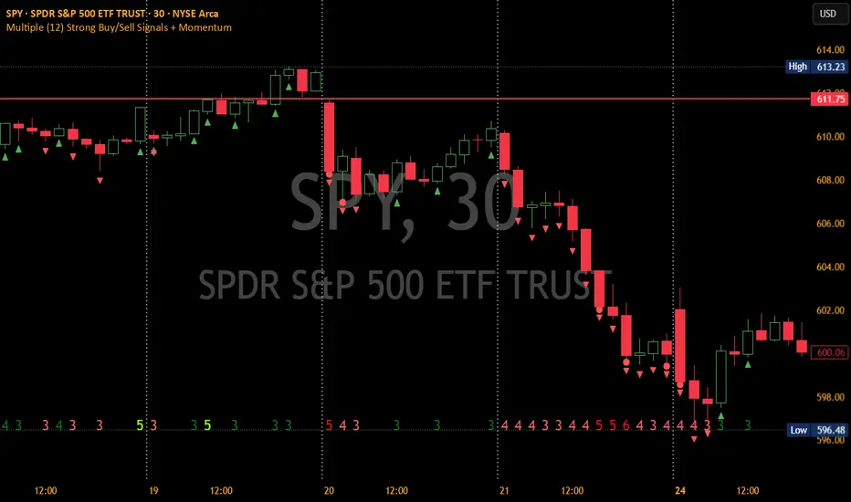
[blackcat] L2 FiboKAMA Adaptive TrendOVERVIEW
The L2 FiboKAMA Adaptive Trend indicator leverages advanced technical analysis techniques by integrating Fibonacci principles with the Kaufman Adaptive Moving Average (KAMA). This combination creates a dynamic and responsive tool designed to adapt seamlessly to changing market conditions. By providing clear buy and sell signals based on adaptive momentum, this indicator helps traders identify potential entry and exit points effectively. Its intuitive design and robust features make it a valuable addition to any trader’s arsenal 📊💹.
According to the principle of Kaufman's Adaptive Moving Average (KAMA), it is a type of moving average line specifically designed for markets with high volatility. Unlike traditional moving averages, KAMA can automatically adjust its period based on market conditions to improve accuracy and responsiveness. This makes it particularly useful for capturing market trends and reducing false signals in varying market environments.
The use of Fibonacci magic numbers (3, 8, 13) enhances the performance and accuracy of KAMA. These numbers have special mathematical properties that align well with the changing trends of KAMA moving averages. Combining them with KAMA can significantly boost its effectiveness, making it a popular choice among traders seeking reliable signals.
This fusion not only smoothens price fluctuations but also ensures quick responses to market changes, offering dependable entry and exit points. Thanks to the flexibility and precision of KAMA combined with Fibonacci magic numbers, traders can better manage risks and aim for higher returns.
FEATURES
Enhanced Kaufman Adaptive Moving Average (KAMA): Incorporates Fibonacci principles for improved adaptability:
Source Price: Allows customization of the price series used for calculation (default: HLCC4).
Fast Length: Determines the period for quicker adjustments to recent price changes.
Slow Length: Sets the period for smoother transitions over longer-term trends.
Dynamic Lines:
KAMA Line: A yellow line representing the primary adaptive moving average, which adapts quickly to new trends.
Trigger Line: A fuchsia line serving as a reference point for detecting crossovers and generating signals.
Visual Cues:
Buy Signals: Green 'B' labels indicating potential buying opportunities.
Sell Signals: Red 'S' labels signaling possible selling points.
Fill Areas: Colored regions between the KAMA and Trigger lines to visually represent trend directions and strength.
Alert Functionality: Generates real-time alerts for both buy and sell signals, ensuring timely notifications for actionable insights 🔔.
Customizable Parameters: Offers flexibility through adjustable inputs, allowing users to tailor the indicator to their specific trading strategies and preferences.
HOW TO USE
Adding the Indicator:
Open your TradingView chart and navigate to the indicators list.
Select L2 FiboKAMA Adaptive Trend and add it to your chart.
Configuring Parameters:
Adjust the Source Price to choose the desired price series (e.g., close, open, high, low).
Set the Fast Length to define how quickly the indicator responds to recent price movements.
Configure the Slow Length to determine the smoothness of long-term trend adaptations.
Interpreting Signals:
Monitor the chart for green 'B' labels indicating buy signals and red 'S' labels for sell signals.
Observe the colored fill areas between the KAMA and Trigger lines to gauge trend strength and direction.
Setting Up Alerts:
Enable alerts within the indicator settings to receive notifications whenever buy or sell signals are triggered.
Customize alert messages and frequencies according to your trading plan.
Combining with Other Tools:
Integrate this indicator with additional technical analysis tools and fundamental research for comprehensive decision-making.
Confirm signals using other indicators like RSI, MACD, or Bollinger Bands for increased reliability.
Optimizing Performance:
Backtest the indicator across various assets and timeframes to understand its behavior under different market conditions.
Fine-tune parameters based on historical performance and current market dynamics.
Integrating Magic Numbers:
Understand the basic principles of KAMA to find suitable entry points for Fibonacci magic numbers.
Utilize the efficiency ratio to measure market volatility and adjust moving average parameters accordingly.
Apply Fibonacci magic numbers (3, 8, 13) to enhance the responsiveness and accuracy of KAMA.
LIMITATIONS
Market Volatility: May produce false signals during periods of extreme volatility or sideways movement.
Parameter Sensitivity: Requires careful tuning of fast and slow lengths to balance responsiveness and stability.
Asset-Specific Behavior: Effectiveness can vary significantly across different financial instruments and time horizons.
Complementary Analysis: Should be used alongside other analytical methods to enhance accuracy and reduce risk.
NOTES
Historical Data: Ensure adequate historical data availability for precise calculations and backtesting.
Demo Testing: Thoroughly test the indicator on demo accounts before deploying it in live trading environments.
Continuous Learning: Stay updated with market trends and continuously refine your strategy incorporating feedback from the indicator's performance.
Risk Management: Always implement proper risk management practices regardless of the signals provided by the indicator.
ADVANCED USAGE TIPS
Multi-Timeframe Analysis: Apply the indicator across multiple timeframes to gain deeper insights into underlying trends.
Divergence Strategy: Look for divergences between price action and the KAMA line to spot potential reversals early.
Volume Integration: Combine volume analysis with the indicator to confirm the strength of identified trends.
Custom Scripting: Modify the script to include additional filters or conditions tailored to your unique trading approach.
IMPROVING KAMA PERFORMANCE
Increase Length: Extend the KAMA length to consider more historical data, reducing the impact of short-term price fluctuations.
Adjust Fast and Slow Lengths: Make KAMA smoother by increasing the fast length and decreasing the slow length.
Use Smoothing Factor: Apply a smoothing factor to control the level of smoothness; typical values range from 0 to 1.
Combine with Other Indicators: Pair KAMA with other smoothing indicators like EMA or SMA for more reliable signals.
Filter Noise: Use filters or other technical analysis tools to eliminate price noise, enhancing KAMA's effectiveness.
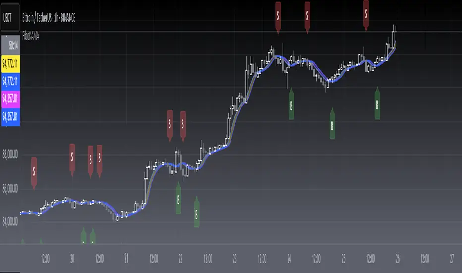
[blackcat] L3 Magic-9 MACD SetupOVERVIEW
The L3 Magic-9 MACD Setup indicator is meticulously crafted to assist traders in identifying precise buy and sell signals through an enhanced Moving Average Convergence Divergence (MACD) methodology. This advanced tool integrates the Magic-9 Sequential technique to refine signal accuracy by filtering out market noise. By providing clear visual cues via labeled charts and real-time alerts, it empowers users to make informed trading decisions swiftly and confidently 📈✅.
FEATURES
Customizable MACD Parameters:
Fast Length: Adjustable parameter to control the sensitivity of the fast moving average.
Slow Length: Configurable setting for the slow moving average to balance responsiveness and stability.
Signal Length: Modifiable value to determine the smoothing factor applied to the MACD line.
Dynamic Plot Visuals:
MACD Line: Representing the difference between short-term and long-term EMAs.
Signal Line: A smoothed version of the MACD line used to generate crossover signals.
Histogram: Illustrating the distance between the MACD and Signal lines, highlighting momentum changes.
All elements feature adjustable colors and styles for personalized visualization preferences 🎨.
Advanced Filtering Mechanism:
Utilizes the Magic-9 Sequential method to analyze consecutive price movements, enhancing signal reliability.
Counts sequential occurrences above or below initial values to detect trends more accurately 🔍.
Sequential Labels:
Displays numerical labels (e.g., '5', '6', etc.) at key points where sequential conditions are met, offering insights into trend strength.
Highlights significant reversals with special labels like '9' and '13' for critical decision-making moments 🏷️.
Buy/Sell Signals:
Generates clear 'B' (buy) and 'S' (sell) labels based on predefined conditions derived from sequential analysis.
Provides actionable trade suggestions directly on the chart for easy interpretation.
Alert System:
Supports customizable alerts to notify users instantly when buy/sell conditions are triggered.
Ensures timely responses to market movements without constant monitoring 🔔.
HOW TO USE
Add Indicator to Chart:
Access the TradingView platform and navigate to the indicators section.
Select ' L3 Magic-9 MACD Setup' from the list and add it to your desired chart.
Configure Settings:
Open the settings panel to adjust MACD parameters such as Fast Length, Slow Length, and Signal Length according to your trading strategy.
Modify plot colors and styles to suit your visual preferences for better readability.
Analyze Chart Labels:
Monitor the chart for sequentially numbered labels indicating trend strength and potential reversal points.
Pay close attention to special labels like '9' and '13' for crucial trading signals.
Combine with Other Tools:
Use additional technical indicators or fundamental analysis to confirm signals generated by the L3 Magic-9 MACD Setup.
Enhance decision-making accuracy by cross-verifying multiple data sources.
LIMITATIONS
Market Conditions Sensitivity:
The indicator may produce fewer reliable signals during periods of low volatility or range-bound markets.
Traders should be cautious of false positives in highly choppy environments 🌪️.
Dependency on Historical Data:
Accurate performance requires sufficient historical price data; insufficient data may lead to inaccurate calculations.
Regular updates and backtesting are essential to maintain effectiveness over time.
Single Indicator Risk:
Relying solely on MACD-based signals can miss broader market context; combining with other analytical tools is recommended.
Always validate signals through multiple lenses to mitigate risks associated with single-indicator strategies.
NOTES
Data Sufficiency:
Ensure your chart has enough historical data loaded to support robust MACD computations.
Periodically review and update data inputs to reflect current market dynamics.
Testing and Validation:
Conduct thorough testing on demo accounts before deploying the indicator in live trading scenarios.
Backtest across various market cycles to assess its resilience under different conditions.
Parameter Optimization:
Experiment with different parameter settings tailored to specific asset classes or trading styles.
Fine-tune the lookback period and other configurable options to align with personal trading objectives.