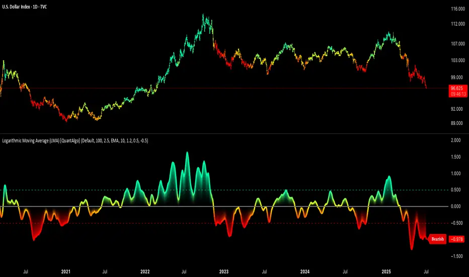
Quick scan for drift🙏🏻
ML based algorading is all about detecting any kind of non-randomness & exploiting it, kinda speculative stuff, not my way, but still...
Drift is one of the patterns that can be exploited, because pure random walks & noise aint got no drift.
This is an efficient method to quickly scan tons of timeseries on the go & detect the ones with drift by simply checking wherther drift < -0.5 or drift > 0.5. The code can be further optimized both in general and for specific needs, but I left it like dat for clarity so you can understand how it works in a minute not in an hour
^^ proving 0.5 and -0.5 are natural limits with no need to optimize anything, we simply put the metric on random noise and see it sits in between -0.5 and 0.5
You can simply take this one and never check anything again if you require numerous live scans on the go. The metric is purely geometrical, no connection to stats, TSA, DSA or whatever. I've tested numerous formulas involving other scaling techniques, drift estimates etc (even made a recursive algo that had a great potential to be written about in a paper, but not this time I gues lol), this one has the highest info gain aka info content.
The timeseries filtered by this lil metric can be further analyzed & modelled with more sophisticated tools.
Live Long and Prosper
P.S.: there's no such thing as polynomial trend/drift, it's alwasy linear, these curves you see are just really long cycles
P.S.: does cheer still work on TV? @admin
Поиск скриптов по запросу "通达信+选股公式+换手率+0.5+源码"
ICT Master Suite [Trading IQ]Hello Traders!
We’re excited to introduce the ICT Master Suite by TradingIQ, a new tool designed to bring together several ICT concepts and strategies in one place.
The Purpose Behind the ICT Master Suite
There are a few challenges traders often face when using ICT-related indicators:
Many available indicators focus on one or two ICT methods, which can limit traders who apply a broader range of ICT related techniques on their charts.
There aren't many indicators for ICT strategy models, and we couldn't find ICT indicators that allow for testing the strategy models and setting alerts.
Many ICT related concepts exist in the public domain as indicators, not strategies! This makes it difficult to verify that the ICT concept has some utility in the market you're trading and if it's worth trading - it's difficult to know if it's working!
Some users might not have enough chart space to apply numerous ICT related indicators, which can be restrictive for those wanting to use multiple ICT techniques simultaneously.
The ICT Master Suite is designed to offer a comprehensive option for traders who want to apply a variety of ICT methods. By combining several ICT techniques and strategy models into one indicator, it helps users maximize their chart space while accessing multiple tools in a single slot.
Additionally, the ICT Master Suite was developed as a strategy . This means users can backtest various ICT strategy models - including deep backtesting. A primary goal of this indicator is to let traders decide for themselves what markets to trade ICT concepts in and give them the capability to figure out if the strategy models are worth trading!
What Makes the ICT Master Suite Different
There are many ICT-related indicators available on TradingView, each offering valuable insights. What the ICT Master Suite aims to do is bring together a wider selection of these techniques into one tool. This includes both key ICT methods and strategy models, allowing traders to test and activate strategies all within one indicator.
Features
The ICT Master Suite offers:
Multiple ICT strategy models, including the 2022 Strategy Model and Unicorn Model, which can be built, tested, and used for live trading.
Calculation and display of key price areas like Breaker Blocks, Rejection Blocks, Order Blocks, Fair Value Gaps, Equal Levels, and more.
The ability to set alerts based on these ICT strategies and key price areas.
A comprehensive, yet practical, all-inclusive ICT indicator for traders.
Customizable Timeframe - Calculate ICT concepts on off-chart timeframes
Unicorn Strategy Model
2022 Strategy Model
Liquidity Raid Strategy Model
OTE (Optimal Trade Entry) Strategy Model
Silver Bullet Strategy Model
Order blocks
Breaker blocks
Rejection blocks
FVG
Strong highs and lows
Displacements
Liquidity sweeps
Power of 3
ICT Macros
HTF previous bar high and low
Break of Structure indications
Market Structure Shift indications
Equal highs and lows
Swings highs and swing lows
Fibonacci TPs and SLs
Swing level TPs and SLs
Previous day high and low TPs and SLs
And much more! An ongoing project!
How To Use
Many traders will already be familiar with the ICT related concepts listed above, and will find using the ICT Master Suite quite intuitive!
Despite this, let's go over the features of the tool in-depth and how to use the tool!
The image above shows the ICT Master Suite with almost all techniques activated.
ICT 2022 Strategy Model
The ICT Master suite provides the ability to test, set alerts for, and live trade the ICT 2022 Strategy Model.
The image above shows an example of a long position being entered following a complete setup for the 2022 ICT model.
A liquidity sweep occurs prior to an upside breakout. During the upside breakout the model looks for the FVG that is nearest 50% of the setup range. A limit order is placed at this FVG for entry.
The target entry percentage for the range is customizable in the settings. For instance, you can select to enter at an FVG nearest 33% of the range, 20%, 66%, etc.
The profit target for the model generally uses the highest high of the range (100%) for longs and the lowest low of the range (100%) for shorts. Stop losses are generally set at 0% of the range.
The image above shows the short model in action!
Whether you decide to follow the 2022 model diligently or not, you can still set alerts when the entry condition is met.
ICT Unicorn Model
The image above shows an example of a long position being entered following a complete setup for the ICT Unicorn model.
A lower swing low followed by a higher swing high precedes the overlap of an FVG and breaker block formed during the sequence.
During the upside breakout the model looks for an FVG and breaker block that formed during the sequence and overlap each other. A limit order is placed at the nearest overlap point to current price.
The profit target for this example trade is set at the swing high and the stop loss at the swing low. However, both the profit target and stop loss for this model are configurable in the settings.
For Longs, the selectable profit targets are:
Swing High
Fib -0.5
Fib -1
Fib -2
For Longs, the selectable stop losses are:
Swing Low
Bottom of FVG or breaker block
The image above shows the short version of the Unicorn Model in action!
For Shorts, the selectable profit targets are:
Swing Low
Fib -0.5
Fib -1
Fib -2
For Shorts, the selectable stop losses are:
Swing High
Top of FVG or breaker block
The image above shows the profit target and stop loss options in the settings for the Unicorn Model.
Optimal Trade Entry (OTE) Model
The image above shows an example of a long position being entered following a complete setup for the OTE model.
Price retraces either 0.62, 0.705, or 0.79 of an upside move and a trade is entered.
The profit target for this example trade is set at the -0.5 fib level. This is also adjustable in the settings.
For Longs, the selectable profit targets are:
Swing High
Fib -0.5
Fib -1
Fib -2
The image above shows the short version of the OTE Model in action!
For Shorts, the selectable profit targets are:
Swing Low
Fib -0.5
Fib -1
Fib -2
Liquidity Raid Model
The image above shows an example of a long position being entered following a complete setup for the Liquidity Raid Modell.
The user must define the session in the settings (for this example it is 13:30-16:00 NY time).
During the session, the indicator will calculate the session high and session low. Following a “raid” of either the session high or session low (after the session has completed) the script will look for an entry at a recently formed breaker block.
If the session high is raided the script will look for short entries at a bearish breaker block. If the session low is raided the script will look for long entries at a bullish breaker block.
For Longs, the profit target options are:
Swing high
User inputted Lib level
For Longs, the stop loss options are:
Swing low
User inputted Lib level
Breaker block bottom
The image above shows the short version of the Liquidity Raid Model in action!
For Shorts, the profit target options are:
Swing Low
User inputted Lib level
For Shorts, the stop loss options are:
Swing High
User inputted Lib level
Breaker block top
Silver Bullet Model
The image above shows an example of a long position being entered following a complete setup for the Silver Bullet Modell.
During the session, the indicator will determine the higher timeframe bias. If the higher timeframe bias is bullish the strategy will look to enter long at an FVG that forms during the session. If the higher timeframe bias is bearish the indicator will look to enter short at an FVG that forms during the session.
For Longs, the profit target options are:
Nearest Swing High Above Entry
Previous Day High
For Longs, the stop loss options are:
Nearest Swing Low
Previous Day Low
The image above shows the short version of the Silver Bullet Model in action!
For Shorts, the profit target options are:
Nearest Swing Low Below Entry
Previous Day Low
For Shorts, the stop loss options are:
Nearest Swing High
Previous Day High
Order blocks
The image above shows indicator identifying and labeling order blocks.
The color of the order blocks, and how many should be shown, are configurable in the settings!
Breaker Blocks
The image above shows indicator identifying and labeling order blocks.
The color of the breaker blocks, and how many should be shown, are configurable in the settings!
Rejection Blocks
The image above shows indicator identifying and labeling rejection blocks.
The color of the rejection blocks, and how many should be shown, are configurable in the settings!
Fair Value Gaps
The image above shows indicator identifying and labeling fair value gaps.
The color of the fair value gaps, and how many should be shown, are configurable in the settings!
Additionally, you can select to only show fair values gaps that form after a liquidity sweep. Doing so reduces "noisy" FVGs and focuses on identifying FVGs that form after a significant trading event.
The image above shows the feature enabled. A fair value gap that occurred after a liquidity sweep is shown.
Market Structure
The image above shows the ICT Master Suite calculating market structure shots and break of structures!
The color of MSS and BoS, and whether they should be displayed, are configurable in the settings.
Displacements
The images above show indicator identifying and labeling displacements.
The color of the displacements, and how many should be shown, are configurable in the settings!
Equal Price Points
The image above shows the indicator identifying and labeling equal highs and equal lows.
The color of the equal levels, and how many should be shown, are configurable in the settings!
Previous Custom TF High/Low
The image above shows the ICT Master Suite calculating the high and low price for a user-defined timeframe. In this case the previous day’s high and low are calculated.
To illustrate the customizable timeframe function, the image above shows the indicator calculating the previous 4 hour high and low.
Liquidity Sweeps
The image above shows the indicator identifying a liquidity sweep prior to an upside breakout.
The image above shows the indicator identifying a liquidity sweep prior to a downside breakout.
The color and aggressiveness of liquidity sweep identification are adjustable in the settings!
Power Of Three
The image above shows the indicator calculating Po3 for two user-defined higher timeframes!
Macros
The image above shows the ICT Master Suite identifying the ICT macros!
ICT Macros are only displayable on the 5 minute timeframe or less.
Strategy Performance Table
In addition to a full-fledged TradingView backtest for any of the ICT strategy models the indicator offers, a quick-and-easy strategy table exists for the indicator!
The image above shows the strategy performance table in action.
Keep in mind that, because the ICT Master Suite is a strategy script, you can perform fully automatic backtests, deep backtests, easily add commission and portfolio balance and look at pertinent metrics for the ICT strategies you are testing!
Lite Mode
Traders who want the cleanest chart possible can toggle on “Lite Mode”!
In Lite Mode, any neon or “glow” like effects are removed and key levels are marked as strict border boxes. You can also select to remove box borders if that’s what you prefer!
Settings Used For Backtest
For the displayed backtest, a starting balance of $1000 USD was used. A commission of 0.02%, slippage of 2 ticks, a verify price for limit orders of 2 ticks, and 5% of capital investment per order.
A commission of 0.02% was used due to the backtested asset being a perpetual future contract for a crypto currency. The highest commission (lowest-tier VIP) for maker orders on many exchanges is 0.02%. All entered positions take place as maker orders and so do profit target exits. Stop orders exist as stop-market orders.
A slippage of 2 ticks was used to simulate more realistic stop-market orders. A verify limit order settings of 2 ticks was also used. Even though BTCUSDT.P on Binance is liquid, we just want the backtest to be on the safe side. Additionally, the backtest traded 100+ trades over the period. The higher the sample size the better; however, this example test can serve as a starting point for traders interested in ICT concepts.
Community Assistance And Feedback
Given the complexity and idiosyncratic applications of ICT concepts amongst its proponents, the ICT Master Suite’s built-in strategies and level identification methods might not align with everyone's interpretation.
That said, the best we can do is precisely define ICT strategy rules and concepts to a repeatable process, test, and apply them! Whether or not an ICT strategy is trading precisely how you would trade it, seeing the model in action, taking trades, and with performance statistics is immensely helpful in assessing predictive utility.
If you think we missed something, you notice a bug, have an idea for strategy model improvement, please let us know! The ICT Master Suite is an ongoing project that will, ideally, be shaped by the community.
A big thank you to the @PineCoders for their Time Library!
Thank you!

Hurst Exponent SmoothedDescription:
The Hurst Exponent Smoothed indicator provides a dynamic analysis of market behavior by calculating the Hurst Exponent over a specified lookback period. This tool is especially useful for identifying whether a market is trending or mean-reverting.
Key Features:
Lookback Period: Set to 90 by default, this parameter controls how many periods the indicator considers for its calculations. Adjusting this value allows you to fine-tune the sensitivity of the indicator to recent price action.
Market Analysis: The Hurst Exponent gives insights into the nature of price movement:
A value near 0.5 suggests a random walk, indicating that the market is unpredictable.
Values above 0.5 indicate a trending market where price movements exhibit persistence, suggesting that the current trend may continue.
Values below 0.5 point to a mean-reverting market, where price movements tend to reverse, making it a potential signal for contrarian trading strategies.
Usage:
Trend Following: When the Hurst Exponent is consistently above 0.5, it may indicate a strong trend. Traders can use this information to align with the current market direction.
Mean Reversion: If the Hurst Exponent falls below 0.5, it could signal that the market is more likely to revert to the mean, offering opportunities for mean-reversion strategies.
Visuals:
The indicator displays a smooth line oscillating between values, giving traders a clear visual cue for the current market condition.
The script is optimized for various timeframes, as demonstrated on the BTCUSD pair on a 270-minute chart. Traders can adapt the lookback period based on their trading style and the specific asset being analyzed.
Open Source: This script is open-source and free to use. Feel free to customize and adapt it to your needs!

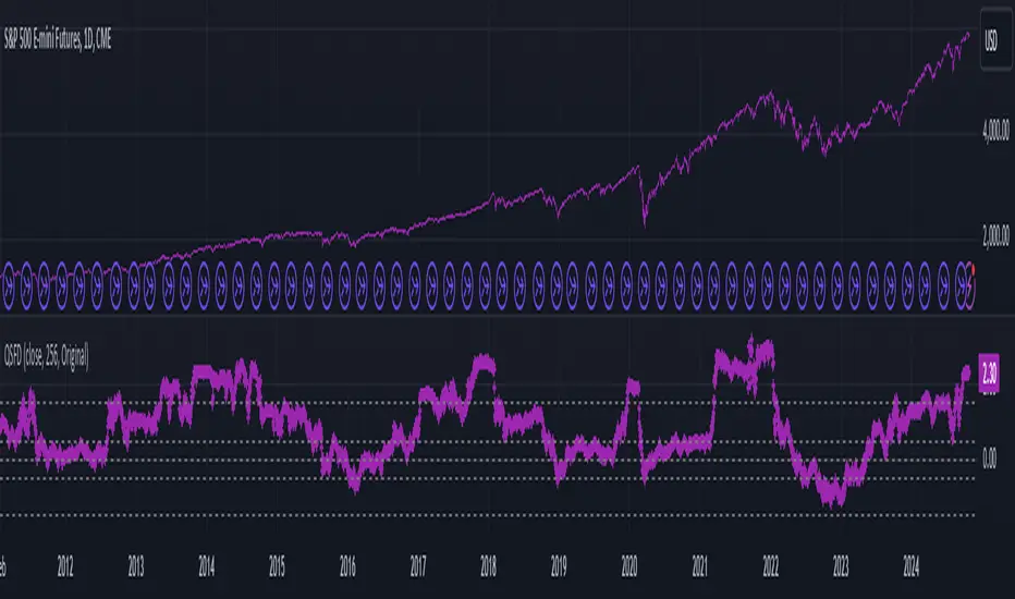
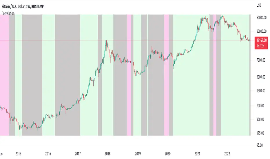
Correlation ZonesThis indicator highlights zones with strong, weak and negative correlation. Unlike standard coefficient indicator it will help to filter out noise when analyzing dependencies between two assets.
With default input setting Correlation_Threshold=0.5:
- Zones with correlation above 0.5, will be colored in green (strong correlation)
- Zones with correlation from -0.5 to 0.5 will be colored grey (weak correlation)
- Zones with correlation below -0.5 will be colore red (strong negative correlation)
Input parameter "Correlation_Threshold" can be modified in settings.
Provided example demonstrates BTCUSD correlation with NASDAQ Composite . I advice to use weekly timeframe and set length to 26 week for this study
Capped Standard Power Option [Loxx]Power options can lead to very high leverage and thus entail potentially very large losses for short positions in these options. It is therefore common to cap the payoff. The maximum payoff is set to some predefined level C. The payoff at maturity for a capped power call is min . Esser (2003) gives the closed-form solution: (via "The Complete Guide to Option Pricing Formulas")
c = S^i * (e^((i - 1) * (r + i*v^2 / 2) - i * (r - b))*T) * (N(e1) - N(e3)) - e^(-r*T) * (X*N(e2) - (C + X) * N(e4))
while the value of a put is
e1 = (log(S/X^(1/i)) + (b + (i - 1/2)*v^2)*T) / v*T^0.5
e3 = (log(S/(C + X)^(1/i)) + (b + (i - 1/2)*v^2)*T) / v*T^0.5
e4 = e3 - i * v * T^0.5
In the case of a capped power put, we have
p = e^(-r*T) * (X*N(-e2) - (C + X) * N(-e4)) - S^i * (e^((i - 1) * (r + i*v^2 / 2) - i * (r - b))*T) * (N(-e1) - N(-e3))
where e1 and e2 is as before. e3 and e4 has to be changed to
e3 = (log(S/(X - C)^(1/i)) + (b + (i - 1/2)*v^2)*T) / v*T^0.5
e4 = e3 - i * v * T^0.5
b=r options on non-dividend paying stock
b=r-q options on stock or index paying a dividend yield of q
b=0 options on futures
b=r-rf currency options (where rf is the rate in the second currency)
Inputs
S = Stock price.
K = Strike price of option.
T = Time to expiration in years.
r = Risk-free rate
c = Cost of Carry
V = Variance of the underlying asset price
i = power
c = Capped on pay off
cnd1(x) = Cumulative Normal Distribution
nd(x) = Standard Normal Density Function
convertingToCCRate(r, cmp ) = Rate compounder
Numerical Greeks or Greeks by Finite Difference
Analytical Greeks are the standard approach to estimating Delta, Gamma etc... That is what we typically use when we can derive from closed form solutions. Normally, these are well-defined and available in text books. Previously, we relied on closed form solutions for the call or put formulae differentiated with respect to the Black Scholes parameters. When Greeks formulae are difficult to develop or tease out, we can alternatively employ numerical Greeks - sometimes referred to finite difference approximations. A key advantage of numerical Greeks relates to their estimation independent of deriving mathematical Greeks. This could be important when we examine American options where there may not technically exist an exact closed form solution that is straightforward to work with. (via VinegarHill FinanceLabs)
Things to know
Only works on the daily timeframe and for the current source price.
You can adjust the text size to fit the screen

3 more indicators: Inverse Fisher on RSI/MFI and CyberCycleSuggested by John Ehlers, IFT helps you to determine the exact oversold/overbought points in any oscillator-type indicators.
The 3 IFT based indicators in this chart are:
- Inverse Fisher on RSI (IFTRSI)
- Inverse Fisher on MFI (IFTMFI)
- Inverse Fisher on CyberCycle (IFTCC)
Suggested method to use any IFT indicator is to buy when the indicator crosses over –0.5 or crosses over +0.5 if it has not previously crossed over –0.5 and to sell short when the indicators crosses under +0.5 or crosses under –0.5 if it has not previously crossed under +0.5.
More info: www.mesasoftware.com
You can use these indicators by doing "Make it mine" (Click on "Share" to open the dialog box with this button).
Let me know what you think, would love to hear how these indicators are used and how effective these are for other instruments.

Fisher (zero-color + simple OB assist)//@version=5
indicator("Fisher (zero-color + simple OB assist)", overlay=false)
// Inputs
length = input.int(10, "Fisher Period", minval=1)
pivotLen = input.int(3, "Structure pivot length (SMC-lite)", minval=1)
showZero = input.bool(true, "Show Zero Line")
colPos = input.color(color.lime, "Color Above 0 (fallback)")
colNeg = input.color(color.red, "Color Below 0 (fallback)")
useOB = input.bool(true, "Color by OB proximity (Demand below = green, Supply above = red)")
showOBMarks = input.bool(true, "Show OB markers")
// Fisher (MT4-style port)
price = (high + low) / 2.0
hh = ta.highest(high, length)
ll = ta.lowest(low, length)
rng = hh - ll
norm = rng != 0 ? (price - ll) / rng : 0.5
var float v = 0.0
var float fish = 0.0
v := 0.33 * 2.0 * (norm - 0.5) + 0.67 * nz(v , 0)
v := math.min(math.max(v, -0.999), 0.999)
fish := 0.5 * math.log((1 + v) / (1 - v)) + 0.5 * nz(fish , 0)
// SMC-lite OB
ph = ta.pivothigh(high, pivotLen, pivotLen)
pl = ta.pivotlow(low, pivotLen, pivotLen)
var float lastSwingHigh = na
var float lastSwingLow = na
if not na(ph)
lastSwingHigh := ph
if not na(pl)
lastSwingLow := pl
bosUp = not na(lastSwingHigh) and close > lastSwingHigh
bosDn = not na(lastSwingLow) and close < lastSwingLow
bearishBar = close < open
bullishBar = close > open
demHigh_new = ta.valuewhen(bearishBar, high, 0)
demLow_new = ta.valuewhen(bearishBar, low, 0)
supHigh_new = ta.valuewhen(bullishBar, high, 0)
supLow_new = ta.valuewhen(bullishBar, low, 0)
// แยกประกาศตัวแปรทีละตัว และใช้ชนิดให้ชัดเจน
var float demHigh = na
var float demLow = na
var float supHigh = na
var float supLow = na
var bool demActive = false
var bool supActive = false
if bosUp and not na(demHigh_new) and not na(demLow_new)
demHigh := demHigh_new
demLow := demLow_new
demActive := true
if bosDn and not na(supHigh_new) and not na(supLow_new)
supHigh := supHigh_new
supLow := supLow_new
supActive := true
// Mitigation (แตะโซน)
if demActive and not na(demHigh) and not na(demLow)
if low <= demHigh
demActive := false
if supActive and not na(supHigh) and not na(supLow)
if high >= supLow
supActive := false
demandBelow = useOB and demActive and not na(demHigh) and demHigh <= close
supplyAbove = useOB and supActive and not na(supLow) and supLow >= close
colDimUp = color.new(colPos, 40)
colDimDown = color.new(colNeg, 40)
barColor = demandBelow ? colPos : supplyAbove ? colNeg : fish > 0 ? colDimUp : colDimDown
// Plots
plot(0, title="Zero", color=showZero ? color.new(color.gray, 70) : color.new(color.gray, 100))
plot(fish, title="Fisher", style=plot.style_columns, color=barColor, linewidth=2)
plotchar(showOBMarks and demandBelow ? fish : na, title="Demand below", char="D", location=location.absolute, color=color.teal, size=size.tiny)
plotchar(showOBMarks and supplyAbove ? fish : na, title="Supply above", char="S", location=location.absolute, color=color.fuchsia, size=size.tiny)
alertcondition(ta.crossover(fish, 0.0), "Fisher Cross Up", "Fisher crosses above 0")
alertcondition(ta.crossunder(fish, 0.0), "Fisher Cross Down", "Fisher crosses below 0")

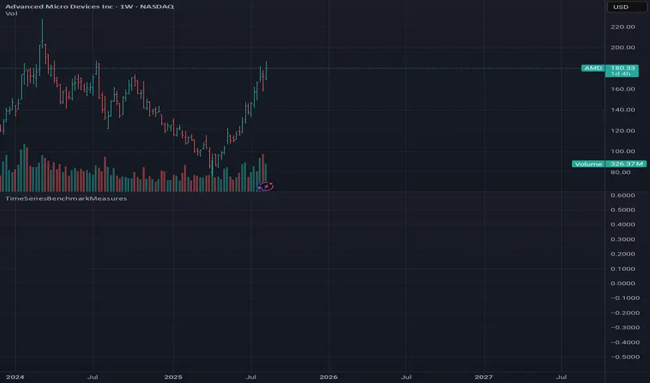
TimeSeriesBenchmarkMeasuresLibrary "TimeSeriesBenchmarkMeasures"
Time Series Benchmark Metrics. \
Provides a comprehensive set of functions for benchmarking time series data, allowing you to evaluate the accuracy, stability, and risk characteristics of various models or strategies. The functions cover a wide range of statistical measures, including accuracy metrics (MAE, MSE, RMSE, NRMSE, MAPE, SMAPE), autocorrelation analysis (ACF, ADF), and risk measures (Theils Inequality, Sharpness, Resolution, Coverage, and Pinball).
___
Reference:
- github.com .
- medium.com .
- www.salesforce.com .
- towardsdatascience.com .
- github.com .
mae(actual, forecasts)
In statistics, mean absolute error (MAE) is a measure of errors between paired observations expressing the same phenomenon. Examples of Y versus X include comparisons of predicted versus observed, subsequent time versus initial time, and one technique of measurement versus an alternative technique of measurement.
Parameters:
actual (array) : List of actual values.
forecasts (array) : List of forecasts values.
Returns: - Mean Absolute Error (MAE).
___
Reference:
- en.wikipedia.org .
- The Orange Book of Machine Learning - Carl McBride Ellis .
mse(actual, forecasts)
The Mean Squared Error (MSE) is a measure of the quality of an estimator. As it is derived from the square of Euclidean distance, it is always a positive value that decreases as the error approaches zero.
Parameters:
actual (array) : List of actual values.
forecasts (array) : List of forecasts values.
Returns: - Mean Squared Error (MSE).
___
Reference:
- en.wikipedia.org .
rmse(targets, forecasts, order, offset)
Calculates the Root Mean Squared Error (RMSE) between target observations and forecasts. RMSE is a standard measure of the differences between values predicted by a model and the values actually observed.
Parameters:
targets (array) : List of target observations.
forecasts (array) : List of forecasts.
order (int) : Model order parameter that determines the starting position in the targets array, `default=0`.
offset (int) : Forecast offset related to target, `default=0`.
Returns: - RMSE value.
nmrse(targets, forecasts, order, offset)
Normalised Root Mean Squared Error.
Parameters:
targets (array) : List of target observations.
forecasts (array) : List of forecasts.
order (int) : Model order parameter that determines the starting position in the targets array, `default=0`.
offset (int) : Forecast offset related to target, `default=0`.
Returns: - NRMSE value.
rmse_interval(targets, forecasts)
Root Mean Squared Error for a set of interval windows. Computes RMSE by converting interval forecasts (with min/max bounds) into point forecasts using the mean of the interval bounds, then compares against actual target values.
Parameters:
targets (array) : List of target observations.
forecasts (matrix) : The forecasted values in matrix format with at least 2 columns (min, max).
Returns: - RMSE value for the combined interval list.
mape(targets, forecasts)
Mean Average Percentual Error.
Parameters:
targets (array) : List of target observations.
forecasts (array) : List of forecasts.
Returns: - MAPE value.
smape(targets, forecasts, mode)
Symmetric Mean Average Percentual Error. Calculates the Mean Absolute Percentage Error (MAPE) between actual targets and forecasts. MAPE is a common metric for evaluating forecast accuracy, expressed as a percentage, lower values indicate a better forecast accuracy.
Parameters:
targets (array) : List of target observations.
forecasts (array) : List of forecasts.
mode (int) : Type of method: default=0:`sum(abs(Fi-Ti)) / sum(Fi+Ti)` , 1:`mean(abs(Fi-Ti) / ((Fi + Ti) / 2))` , 2:`mean(abs(Fi-Ti) / (abs(Fi) + abs(Ti))) * 100`
Returns: - SMAPE value.
mape_interval(targets, forecasts)
Mean Average Percentual Error for a set of interval windows.
Parameters:
targets (array) : List of target observations.
forecasts (matrix) : The forecasted values in matrix format with at least 2 columns (min, max).
Returns: - MAPE value for the combined interval list.
acf(data, k)
Autocorrelation Function (ACF) for a time series at a specified lag.
Parameters:
data (array) : Sample data of the observations.
k (int) : The lag period for which to calculate the autocorrelation. Must be a non-negative integer.
Returns: - The autocorrelation value at the specified lag, ranging from -1 to 1.
___
The autocorrelation function measures the linear dependence between observations in a time series
at different time lags. It quantifies how well the series correlates with itself at different
time intervals, which is useful for identifying patterns, seasonality, and the appropriate
lag structure for time series models.
ACF values close to 1 indicate strong positive correlation, values close to -1 indicate
strong negative correlation, and values near 0 indicate no linear correlation.
___
Reference:
- statisticsbyjim.com
acf_multiple(data, k)
Autocorrelation function (ACF) for a time series at a set of specified lags.
Parameters:
data (array) : Sample data of the observations.
k (array) : List of lag periods for which to calculate the autocorrelation. Must be a non-negative integer.
Returns: - List of ACF values for provided lags.
___
The autocorrelation function measures the linear dependence between observations in a time series
at different time lags. It quantifies how well the series correlates with itself at different
time intervals, which is useful for identifying patterns, seasonality, and the appropriate
lag structure for time series models.
ACF values close to 1 indicate strong positive correlation, values close to -1 indicate
strong negative correlation, and values near 0 indicate no linear correlation.
___
Reference:
- statisticsbyjim.com
adfuller(data, n_lag, conf)
: Augmented Dickey-Fuller test for stationarity.
Parameters:
data (array) : Data series.
n_lag (int) : Maximum lag.
conf (string) : Confidence Probability level used to test for critical value, (`90%`, `95%`, `99%`).
Returns: - `adf` The test statistic.
- `crit` Critical value for the test statistic at the 10 % levels.
- `nobs` Number of observations used for the ADF regression and calculation of the critical values.
___
The Augmented Dickey-Fuller test is used to determine whether a time series is stationary
or contains a unit root (non-stationary). The null hypothesis is that the series has a unit root
(is non-stationary), while the alternative hypothesis is that the series is stationary.
A stationary time series has statistical properties that do not change over time, making it
suitable for many time series forecasting models. If the test statistic is less than the
critical value, we reject the null hypothesis and conclude the series is stationary.
___
Reference:
- www.jstor.org
- en.wikipedia.org
theils_inequality(targets, forecasts)
Calculates Theil's Inequality Coefficient, a measure of forecast accuracy that quantifies the relative difference between actual and predicted values.
Parameters:
targets (array) : List of target observations.
forecasts (array) : Matrix with list of forecasts, ordered column wise.
Returns: - Theil's Inequality Coefficient value, value closer to 0 is better.
___
Theil's Inequality Coefficient is calculated as: `sqrt(Sum((y_i - f_i)^2)) / (sqrt(Sum(y_i^2)) + sqrt(Sum(f_i^2)))`
where `y_i` represents actual values and `f_i` represents forecast values.
This metric ranges from 0 to infinity, with 0 indicating perfect forecast accuracy.
___
Reference:
- en.wikipedia.org
sharpness(forecasts)
The average width of the forecast intervals across all observations, representing the sharpness or precision of the predictive intervals.
Parameters:
forecasts (matrix) : The forecasted values in matrix format with at least 2 columns (min, max).
Returns: - Sharpness The sharpness level, which is the average width of all prediction intervals across the forecast horizon.
___
Sharpness is an important metric for evaluating forecast quality. It measures how narrow or wide the
prediction intervals are. Higher sharpness (narrower intervals) indicates greater precision in the
forecast intervals, while lower sharpness (wider intervals) suggests less precision.
The sharpness metric is calculated as the mean of the interval widths across all observations, where
each interval width is the difference between the upper and lower bounds of the prediction interval.
Note: This function assumes that the forecasts matrix has at least 2 columns, with the first column
representing the lower bounds and the second column representing the upper bounds of prediction intervals.
___
Reference:
- Hyndman, R. J., & Athanasopoulos, G. (2018). Forecasting: principles and practice. OTexts. otexts.com
resolution(forecasts)
Calculates the resolution of forecast intervals, measuring the average absolute difference between individual forecast interval widths and the overall sharpness measure.
Parameters:
forecasts (matrix) : The forecasted values in matrix format with at least 2 columns (min, max).
Returns: - The average absolute difference between individual forecast interval widths and the overall sharpness measure, representing the resolution of the forecasts.
___
Resolution is a key metric for evaluating forecast quality that measures the consistency of prediction
interval widths. It quantifies how much the individual forecast intervals vary from the average interval
width (sharpness). High resolution indicates that the forecast intervals are relatively consistent
across observations, while low resolution suggests significant variation in interval widths.
The resolution is calculated as the mean absolute deviation of individual interval widths from the
overall sharpness value. This provides insight into the uniformity of the forecast uncertainty
estimates across the forecast horizon.
Note: This function requires the forecasts matrix to have at least 2 columns (min, max) representing
the lower and upper bounds of prediction intervals.
___
Reference:
- (sites.stat.washington.edu)
- (www.jstor.org)
coverage(targets, forecasts)
Calculates the coverage probability, which is the percentage of target values that fall within the corresponding forecasted prediction intervals.
Parameters:
targets (array) : List of target values.
forecasts (matrix) : The forecasted values in matrix format with at least 2 columns (min, max).
Returns: - Percent of target values that fall within their corresponding forecast intervals, expressed as a decimal value between 0 and 1 (or 0% and 100%).
___
Coverage probability is a crucial metric for evaluating the reliability of prediction intervals.
It measures how well the forecast intervals capture the actual observed values. An ideal forecast
should have a coverage probability close to the nominal confidence level (e.g., 90%, 95%, or 99%).
For example, if a 95% prediction interval is used, we expect approximately 95% of the actual
target values to fall within those intervals. If the coverage is significantly lower than the
nominal level, the intervals may be too narrow; if it's significantly higher, the intervals may
be too wide.
Note: This function requires the targets array and forecasts matrix to have the same number of
observations, and the forecasts matrix must have at least 2 columns (min, max) representing
the lower and upper bounds of prediction intervals.
___
Reference:
- (www.jstor.org)
pinball(tau, target, forecast)
Pinball loss function, measures the asymmetric loss for quantile forecasts.
Parameters:
tau (float) : The quantile level (between 0 and 1), where 0.5 represents the median.
target (float) : The actual observed value to compare against.
forecast (float) : The forecasted value.
Returns: - The Pinball loss value, which quantifies the distance between the forecast and target relative to the specified quantile level.
___
The Pinball loss function is specifically designed for evaluating quantile forecasts. It is
asymmetric, meaning it penalizes underestimates and overestimates differently depending on the
quantile level being evaluated.
For a given quantile τ, the loss function is defined as:
- If target >= forecast: (target - forecast) * τ
- If target < forecast: (forecast - target) * (1 - τ)
This loss function is commonly used in quantile regression and probabilistic forecasting
to evaluate how well forecasts capture specific quantiles of the target distribution.
___
Reference:
- (www.otexts.com)
pinball_mean(tau, targets, forecasts)
Calculates the mean pinball loss for quantile regression.
Parameters:
tau (float) : The quantile level (between 0 and 1), where 0.5 represents the median.
targets (array) : The actual observed values to compare against.
forecasts (matrix) : The forecasted values in matrix format with at least 2 columns (min, max).
Returns: - The mean pinball loss value across all observations.
___
The pinball_mean() function computes the average Pinball loss across multiple observations,
making it suitable for evaluating overall forecast performance in quantile regression tasks.
This function leverages the asymmetric Pinball loss function to evaluate how well forecasts
capture specific quantiles of the target distribution. The choice of which column from the
forecasts matrix to use depends on the quantile level:
- For τ ≤ 0.5: Uses the first column (min) of forecasts
- For τ > 0.5: Uses the second column (max) of forecasts
This loss function is commonly used in quantile regression and probabilistic forecasting
to evaluate how well forecasts capture specific quantiles of the target distribution.
___
Reference:
- (www.otexts.com)
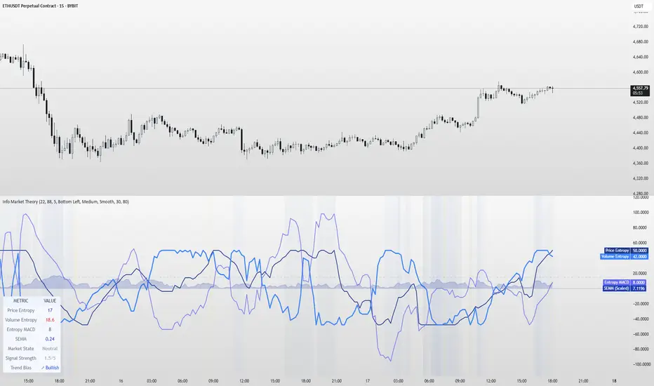
Information Theory Market AnalysisINFORMATION THEORY MARKET ANALYSIS
OVERVIEW
This indicator applies mathematical concepts from information theory to analyze market behavior, measuring the randomness and predictability of price and volume movements through entropy calculations. Unlike traditional technical indicators, it provides insight into market structure and regime changes.
KEY COMPONENTS
Four Main Signals:
• Price Entropy (Deep Blue): Measures randomness in price movements
• Volume Entropy (Bright Blue): Analyzes volume pattern predictability
• Entropy MACD (Purple): Shows relationship between price and volume entropy
• SEMM (Royal Blue): Stochastic Entropy Market Monitor - overall market randomness gauge
Market State Detection:
The indicator identifies seven distinct market states:
• Strong Trending (SEMM < 0.1)
• Weak Trending (0.1-0.2)
• Neutral (0.2-0.3)
• Moderate Random (0.3-0.5)
• High Randomness (0.5-0.8)
• Very Random (0.8-1.0)
• Chaotic (>1.0)
KEY FEATURES
Advanced Analytics:
• Signal Strength Confluence: 0-5 scale measuring alignment of multiple factors
• Entropy Crossovers: Detects shifts between accumulation and distribution phases
• Extreme Readings: Identifies statistical outliers for potential reversals
• Trend Bias Analysis: Directional momentum assessment
Information Dashboard:
• Real-time entropy values and market state
• Signal strength indicator with visual highlighting
• Trend bias with directional arrows
• Color-coded alerts for extreme conditions
Customizable Display:
• Adjustable SEMM scaling (5x to 100x) for optimal visibility
• Multiple line styles: Smooth, Stepped, Dotted
• 9 table positions with 3 size options
• Professional blue color scheme with transparency controls
Comprehensive Alert System - 15 Alert Types Including:
• Extreme entropy readings (price/volume)
• Crossover signals (dominance shifts)
• Market state changes (trending ↔ random)
• High confluence signals (3+ factors aligned)
HOW TO USE
Reading the Signals:
• Entropy Values > ±25: Strong structural signals
• Entropy Values > ±40: Extreme readings, potential reversals
• SEMM < 0.2: Trending market favors directional strategies
• SEMM > 0.5: Random market favors range/scalping strategies
Signal Confluence:
Look for multiple factors aligning:
• Signal Strength ≥ 3.0 for higher probability setups
• Background highlighting indicates confluence
• Table shows real-time strength assessment
Timeframe Optimization:
• Short-term (1m-15m): Entropy Length 14-22, Sensitivity 3-5
• Swing Trading (1H-4H): Default settings optimal
• Position Trading (Daily+): Entropy Length 34-55, Sensitivity 8-12
EDUCATIONAL APPLICATIONS
Market Structure Analysis:
• Understand when markets are trending vs. ranging
• Identify accumulation and distribution phases
• Recognize extreme market conditions
• Measure information content in price movements
Information Theory Concepts:
• Binary entropy calculations applied to financial data
• Probability distribution analysis of returns
• Statistical ranking and percentile analysis
• Momentum-adjusted randomness measurement
TECHNICAL DETAILS
Calculations:
• Uses binary entropy formula: -
• Percentile ranking across multiple timeframes
• Volume-weighted probability distributions
• RSI-adjusted momentum entropy (SEMM)
Customization Options:
• Entropy Length: 5-100 bars (default: 22)
• Average Length: 10-200 bars (default: 88)
• Sensitivity: 1.0-20.0 (default: 5.0, lower = more sensitive)
• SEMM Scaling: 5.0-100.0x (default: 30.0)
IMPORTANT NOTES
Risk Considerations:
• Indicator measures probabilities, not certainties
• High SEMM values (>0.5) suggest increased market randomness
• Extreme readings may persist longer than expected
• Always combine with proper risk management
Educational Purpose:
This indicator is designed for:
• Market structure analysis and education
• Understanding information theory applications in finance
• Developing probabilistic thinking about markets
• Research and analytical purposes
Performance Tips:
• Allow 200+ bars for proper initialization
• Adjust scaling and transparency for optimal visibility
• Use confluence signals for higher probability analysis
• Consider multiple timeframes for comprehensive analysis
DISCLAIMER
This indicator is for educational and analytical purposes. It does not constitute financial advice. Past performance does not guarantee future results. Always conduct your own research and consider your risk tolerance before making trading decisions.
Version: 5.0
Category: Oscillators, Volume, Market Structure
Best For: All timeframes, trending and ranging markets
Complexity: Intermediate to Advanced
SMC Structures and FVGสวัสดีครับ! ผมจะอธิบายอินดิเคเตอร์ "SMC Structures and FVG + MACD" ที่คุณให้มาอย่างละเอียดในแต่ละส่วน เพื่อให้คุณเข้าใจการทำงานของมันอย่างถ่องแท้ครับ
อินดิเคเตอร์นี้เป็นการผสมผสานแนวคิดของ Smart Money Concept (SMC) ซึ่งเน้นการวิเคราะห์โครงสร้างตลาด (Market Structure) และ Fair Value Gap (FVG) เข้ากับอินดิเคเตอร์ MACD เพื่อใช้เป็นตัวกรองหรือตัวยืนยันสัญญาณ Choch/BoS (Change of Character / Break of Structure)
1. ภาพรวมอินดิเคเตอร์ (Overall Purpose)
อินดิเคเตอร์นี้มีจุดประสงค์หลักคือ:
ระบุโครงสร้างตลาด: ตีเส้นและป้ายกำกับ Choch (Change of Character) และ BoS (Break of Structure) บนกราฟโดยอัตโนมัติ
ผสานการยืนยันด้วย MACD: สัญญาณ Choch/BoS จะถูกพิจารณาก็ต่อเมื่อ MACD Histogram เกิดการตัดขึ้นหรือลง (Zero Cross) ในทิศทางที่สอดคล้องกัน
แสดง Fair Value Gap (FVG): หากเปิดใช้งาน จะมีการตีกล่อง FVG บนกราฟ
แสดงระดับ Fibonacci: คำนวณและแสดงระดับ Fibonacci ที่สำคัญตามโครงสร้างตลาดปัจจุบัน
ปรับตาม Timeframe: การคำนวณและการแสดงผลทั้งหมดจะปรับตาม Timeframe ที่คุณกำลังใช้งานอยู่โดยอัตโนมัติ
2. ส่วนประกอบหลักของโค้ด (Code Breakdown)
โค้ดนี้สามารถแบ่งออกเป็นส่วนหลัก ๆ ได้ดังนี้:
2.1 Inputs (การตั้งค่า)
ส่วนนี้คือตัวแปรที่คุณสามารถปรับแต่งได้ในหน้าต่างการตั้งค่าของอินดิเคเตอร์ (คลิกที่รูปฟันเฟืองข้างชื่ออินดิเคเตอร์บนกราฟ)
MACD Settings (ตั้งค่า MACD):
fast_len: ความยาวของ Fast EMA สำหรับ MACD (ค่าเริ่มต้น 12)
slow_len: ความยาวของ Slow EMA สำหรับ MACD (ค่าเริ่มต้น 26)
signal_len: ความยาวของ Signal Line สำหรับ MACD (ค่าเริ่มต้น 9)
= ta.macd(close, fast_len, slow_len, signal_len): คำนวณค่า MACD Line, Signal Line และ Histogram โดยใช้ราคาปิด (close) และค่าความยาวที่กำหนด
is_bullish_macd_cross: ตรวจสอบว่า MACD Histogram ตัดขึ้นเหนือเส้น 0 (จากค่าลบเป็นบวก)
is_bearish_macd_cross: ตรวจสอบว่า MACD Histogram ตัดลงใต้เส้น 0 (จากค่าบวกเป็นลบ)
Fear Value Gap (FVG) Settings:
isFvgToShow: (Boolean) เปิด/ปิดการแสดง FVG บนกราฟ
bullishFvgColor: สีสำหรับ Bullish FVG
bearishFvgColor: สีสำหรับ Bearish FVG
mitigatedFvgColor: สีสำหรับ FVG ที่ถูก Mitigate (ลดทอน) แล้ว
fvgHistoryNbr: จำนวน FVG ย้อนหลังที่จะแสดง
isMitigatedFvgToReduce: (Boolean) เปิด/ปิดการลดขนาด FVG เมื่อถูก Mitigate
Structures (โครงสร้างตลาด) Settings:
isStructBodyCandleBreak: (Boolean) หากเป็น true การ Break จะต้องเกิดขึ้นด้วย เนื้อเทียน ที่ปิดเหนือ/ใต้ Swing High/Low หากเป็น false แค่ไส้เทียนทะลุก็ถือว่า Break
isCurrentStructToShow: (Boolean) เปิด/ปิดการแสดงเส้นโครงสร้างตลาดปัจจุบัน (เส้นสีน้ำเงินในภาพตัวอย่าง)
pivot_len: ความยาวของแท่งเทียนที่ใช้ในการมองหาจุด Pivot (Swing High/Low) ยิ่งค่าน้อยยิ่งจับ Swing เล็กๆ ได้, ยิ่งค่ามากยิ่งจับ Swing ใหญ่ๆ ได้
bullishBosColor, bearishBosColor: สีสำหรับเส้นและป้าย BOS ขาขึ้น/ขาลง
bosLineStyleOption, bosLineWidth: สไตล์ (Solid, Dotted, Dashed) และความหนาของเส้น BOS
bullishChochColor, bearishChochColor: สีสำหรับเส้นและป้าย CHoCH ขาขึ้น/ขาลง
chochLineStyleOption, chochLineWidth: สไตล์ (Solid, Dotted, Dashed) และความหนาของเส้น CHoCH
currentStructColor, currentStructLineStyleOption, currentStructLineWidth: สี, สไตล์ และความหนาของเส้นโครงสร้างตลาดปัจจุบัน
structHistoryNbr: จำนวนการ Break (Choch/BoS) ย้อนหลังที่จะแสดง
Structure Fibonacci (จากโค้ดต้นฉบับ):
เป็นชุด Input สำหรับเปิด/ปิด, กำหนดค่า, สี, สไตล์ และความหนาของเส้น Fibonacci Levels ต่างๆ (0.786, 0.705, 0.618, 0.5, 0.382) ที่จะถูกคำนวณจากโครงสร้างตลาดปัจจุบัน
2.2 Helper Functions (ฟังก์ชันช่วยทำงาน)
getLineStyle(lineOption): ฟังก์ชันนี้ใช้แปลงค่า String ที่เลือกจาก Input (เช่น "─", "┈", "╌") ให้เป็นรูปแบบ line.style_ ที่ Pine Script เข้าใจ
get_structure_highest_bar(lookback): ฟังก์ชันนี้พยายามหา Bar Index ของแท่งเทียนที่ทำ Swing High ภายในช่วง lookback ที่กำหนด
get_structure_lowest_bar(lookback): ฟังก์ชันนี้พยายามหา Bar Index ของแท่งเทียนที่ทำ Swing Low ภายในช่วง lookback ที่กำหนด
is_structure_high_broken(...): ฟังก์ชันนี้ตรวจสอบว่าราคาปัจจุบันได้ Break เหนือ _structureHigh (Swing High) หรือไม่ โดยพิจารณาจาก _highStructBreakPrice (ราคาปิดหรือราคา High ขึ้นอยู่กับการตั้งค่า isStructBodyCandleBreak)
FVGDraw(...): ฟังก์ชันนี้รับ Arrays ของ FVG Boxes, Types, Mitigation Status และ Labels มาประมวลผล เพื่ออัปเดตสถานะของ FVG (เช่น ถูก Mitigate หรือไม่) และปรับขนาด/ตำแหน่งของ FVG Box และ Label บนกราฟ
2.3 Global Variables (ตัวแปรทั่วทั้งอินดิเคเตอร์)
เป็นตัวแปรที่ประกาศด้วย var ซึ่งหมายความว่าค่าของมันจะถูกเก็บไว้และอัปเดตในแต่ละแท่งเทียน (persists across bars)
structureLines, structureLabels: Arrays สำหรับเก็บอ็อบเจกต์ line และ label ของเส้น Choch/BoS ที่วาดบนกราฟ
fvgBoxes, fvgTypes, fvgLabels, isFvgMitigated: Arrays สำหรับเก็บข้อมูลของ FVG Boxes และสถานะต่างๆ
structureHigh, structureLow: เก็บราคาของ Swing High/Low ที่สำคัญของโครงสร้างตลาดปัจจุบัน
structureHighStartIndex, structureLowStartIndex: เก็บ Bar Index ของจุดเริ่มต้นของ Swing High/Low ที่สำคัญ
structureDirection: เก็บสถานะของทิศทางโครงสร้างตลาด (1 = Bullish, 2 = Bearish, 0 = Undefined)
fiboXPrice, fiboXStartIndex, fiboXLine, fiboXLabel: ตัวแปรสำหรับเก็บข้อมูลและอ็อบเจกต์ของเส้น Fibonacci Levels
isBOSAlert, isCHOCHAlert: (Boolean) ใช้สำหรับส่งสัญญาณ Alert (หากมีการตั้งค่า Alert ไว้)
2.4 FVG Processing (การประมวลผล FVG)
ส่วนนี้จะตรวจสอบเงื่อนไขการเกิด FVG (Bullish FVG: high < low , Bearish FVG: low > high )
หากเกิด FVG และ isFvgToShow เป็น true จะมีการสร้าง box และ label ใหม่เพื่อแสดง FVG บนกราฟ
มีการจัดการ fvgBoxes และ fvgLabels เพื่อจำกัดจำนวน FVG ที่แสดงตาม fvgHistoryNbr และลบ FVG เก่าออก
ฟังก์ชัน FVGDraw จะถูกเรียกเพื่ออัปเดตสถานะของ FVG (เช่น การถูก Mitigate) และปรับการแสดงผล
2.5 Structures Processing (การประมวลผลโครงสร้างตลาด)
Initialization: ที่ bar_index == 0 (แท่งเทียนแรกของกราฟ) จะมีการกำหนดค่าเริ่มต้นให้กับ structureHigh, structureLow, structureHighStartIndex, structureLowStartIndex
Finding Current High/Low: highest, highestBar, lowest, lowestBar ถูกใช้เพื่อหา High/Low ที่สุดและ Bar Index ของมันใน 10 แท่งล่าสุด (หรือทั้งหมดหากกราฟสั้นกว่า 10 แท่ง)
Calculating Structure Max/Min Bar: structureMaxBar และ structureMinBar ใช้ฟังก์ชัน get_structure_highest_bar และ get_structure_lowest_bar เพื่อหา Bar Index ของ Swing High/Low ที่แท้จริง (ไม่ใช่แค่ High/Low ที่สุดใน lookback แต่เป็นจุด Pivot ที่สมบูรณ์)
Break Price: lowStructBreakPrice และ highStructBreakPrice จะเป็นราคาปิด (close) หรือราคา Low/High ขึ้นอยู่กับ isStructBodyCandleBreak
isStuctureLowBroken / isStructureHighBroken: เงื่อนไขเหล่านี้ตรวจสอบว่าราคาได้ทำลาย structureLow หรือ structureHigh หรือไม่ โดยพิจารณาจากราคา Break, ราคาแท่งก่อนหน้า และ Bar Index ของจุดเริ่มต้นโครงสร้าง
Choch/BoS Logic (ส่วนสำคัญที่ถูกผสานกับ MACD):
if(isStuctureLowBroken and is_bearish_macd_cross): นี่คือจุดที่ MACD เข้ามามีบทบาท หากราคาทำลาย structureLow (สัญญาณขาลง) และ MACD Histogram เกิด Bearish Zero Cross (is_bearish_macd_cross เป็น true) อินดิเคเตอร์จะพิจารณาว่าเป็น Choch หรือ BoS
หาก structureDirection == 1 (เดิมเป็นขาขึ้น) หรือ 0 (ยังไม่กำหนด) จะตีเป็น "CHoCH" (เปลี่ยนทิศทางโครงสร้างเป็นขาลง)
หาก structureDirection == 2 (เดิมเป็นขาลง) จะตีเป็น "BOS" (ยืนยันโครงสร้างขาลง)
มีการสร้าง line.new และ label.new เพื่อวาดเส้นและป้ายกำกับ
structureDirection จะถูกอัปเดตเป็น 1 (Bullish)
structureHighStartIndex, structureLowStartIndex, structureHigh, structureLow จะถูกอัปเดตเพื่อกำหนดโครงสร้างใหม่
else if(isStructureHighBroken and is_bullish_macd_cross): เช่นกันสำหรับขาขึ้น หากราคาทำลาย structureHigh (สัญญาณขาขึ้น) และ MACD Histogram เกิด Bullish Zero Cross (is_bullish_macd_cross เป็น true) อินดิเคเตอร์จะพิจารณาว่าเป็น Choch หรือ BoS
หาก structureDirection == 2 (เดิมเป็นขาลง) หรือ 0 (ยังไม่กำหนด) จะตีเป็น "CHoCH" (เปลี่ยนทิศทางโครงสร้างเป็นขาขึ้น)
หาก structureDirection == 1 (เดิมเป็นขาขึ้น) จะตีเป็น "BOS" (ยืนยันโครงสร้างขาขึ้น)
มีการสร้าง line.new และ label.new เพื่อวาดเส้นและป้ายกำกับ
structureDirection จะถูกอัปเดตเป็น 2 (Bearish)
structureHighStartIndex, structureLowStartIndex, structureHigh, structureLow จะถูกอัปเดตเพื่อกำหนดโครงสร้างใหม่
การลบเส้นเก่า: d.delete_line (หากไลบรารีทำงาน) จะถูกเรียกเพื่อลบเส้นและป้ายกำกับเก่าออกเมื่อจำนวนเกิน structHistoryNbr
Updating Structure High/Low (else block): หากไม่มีการ Break เกิดขึ้น แต่ราคาปัจจุบันสูงกว่า structureHigh หรือต่ำกว่า structureLow ในทิศทางที่สอดคล้องกัน (เช่น ยังคงเป็นขาขึ้นและทำ High ใหม่) structureHigh หรือ structureLow จะถูกอัปเดตเพื่อติดตาม High/Low ที่สุดของโครงสร้างปัจจุบัน
Current Structure Display:
หาก isCurrentStructToShow เป็น true อินดิเคเตอร์จะวาดเส้น structureHighLine และ structureLowLine เพื่อแสดงขอบเขตของโครงสร้างตลาดปัจจุบัน
Fibonacci Display:
หาก isFiboXToShow เป็น true อินดิเคเตอร์จะคำนวณและวาดเส้น Fibonacci Levels ต่างๆ (0.786, 0.705, 0.618, 0.5, 0.382) โดยอิงจาก structureHigh และ structureLow ของโครงสร้างตลาดปัจจุบัน
Alerts:
alertcondition: ใช้สำหรับตั้งค่า Alert ใน TradingView เมื่อเกิดสัญญาณ BOS หรือ CHOCH
plot(na):
plot(na) เป็นคำสั่งที่สำคัญในอินดิเคเตอร์ที่ไม่ได้ต้องการพล็อต Series ของข้อมูลบนกราฟ (เช่น ไม่ได้พล็อตเส้น EMA หรือ RSI) แต่ใช้วาดอ็อบเจกต์ (Line, Label, Box) โดยตรง
การมี plot(na) ช่วยให้ Pine Script รู้ว่าอินดิเคเตอร์นี้มีเอาต์พุตที่แสดงผลบนกราฟ แม้ว่าจะไม่ได้เป็น Series ที่พล็อตตามปกติก็ตาม
3. วิธีใช้งาน
คัดลอกโค้ดทั้งหมด ที่อยู่ในบล็อก immersive ด้านบน
ไปที่ TradingView และเปิดกราฟที่คุณต้องการ
คลิกที่เมนู "Pine Editor" ที่อยู่ด้านล่างของหน้าจอ
ลบโค้ดเดิมที่มีอยู่ และ วางโค้ดที่คัดลอกมา ลงไปแทน
คลิกที่ปุ่ม "Add to Chart"
อินดิเคเตอร์จะถูกเพิ่มลงในกราฟของคุณโดยอัตโนมัติ คุณสามารถคลิกที่รูปฟันเฟืองข้างชื่ออินดิเคเตอร์บนกราฟเพื่อเข้าถึงหน้าต่างการตั้งค่าและปรับแต่งตามความต้องการของคุณได้
Hello! I will explain the "SMC Structures and FVG + MACD" indicator you provided in detail, section by section, so you can fully understand how it works.This indicator combines the concepts of Smart Money Concept (SMC), which focuses on analyzing Market Structure and Fair Value Gaps (FVG), with the MACD indicator to serve as a filter or confirmation for Choch (Change of Character) and BoS (Break of Structure) signals.1. Overall PurposeThe main purposes of this indicator are:Identify Market Structure: Automatically draw lines and label Choch (Change of Character) and BoS (Break of Structure) on the chart.Integrate MACD Confirmation: Choch/BoS signals will only be considered when the MACD Histogram performs a cross (Zero Cross) in the corresponding direction.Display Fair Value Gap (FVG): If enabled, FVG boxes will be drawn on the chart.Display Fibonacci Levels: Calculate and display important Fibonacci levels based on the current market structure.Adapt to Timeframe: All calculations and displays will automatically adjust to the timeframe you are currently using.2. Code BreakdownThis code can be divided into the following main sections:2.1 Inputs (Settings)This section contains variables that you can adjust in the indicator's settings window (click the gear icon next to the indicator's name on the chart).MACD Settings:fast_len: Length of the Fast EMA for MACD (default 12)slow_len: Length of the Slow EMA for MACD (default 26)signal_len: Length of the Signal Line for MACD (default 9) = ta.macd(close, fast_len, slow_len, signal_len): Calculates the MACD Line, Signal Line, and Histogram using the closing price (close) and the specified lengths.is_bullish_macd_cross: Checks if the MACD Histogram crosses above the 0 line (from negative to positive).is_bearish_macd_cross: Checks if the MACD Histogram crosses below the 0 line (from positive to negative).Fear Value Gap (FVG) Settings:isFvgToShow: (Boolean) Enables/disables the display of FVG on the chart.bullishFvgColor: Color for Bullish FVG.bearishFvgColor: Color for Bearish FVG.mitigatedFvgColor: Color for FVG that has been mitigated.fvgHistoryNbr: Number of historical FVG to display.isMitigatedFvgToReduce: (Boolean) Enables/disables reducing the size of FVG when mitigated.Structures (โครงสร้างตลาด) Settings:isStructBodyCandleBreak: (Boolean) If true, the break must occur with the candle body closing above/below the Swing High/Low. If false, a wick break is sufficient.isCurrentStructToShow: (Boolean) Enables/disables the display of the current market structure lines (blue lines in the example image).pivot_len: Lookback length for identifying Pivot points (Swing High/Low). A smaller value captures smaller, more frequent swings; a larger value captures larger, more significant swings.bullishBosColor, bearishBosColor: Colors for bullish/bearish BOS lines and labels.bosLineStyleOption, bosLineWidth: Style (Solid, Dotted, Dashed) and width of BOS lines.bullishChochColor, bearishChochColor: Colors for bullish/bearish CHoCH lines and labels.chochLineStyleOption, chochLineWidth: Style (Solid, Dotted, Dashed) and width of CHoCH lines.currentStructColor, currentStructLineStyleOption, currentStructLineWidth: Color, style, and width of the current market structure lines.structHistoryNbr: Number of historical breaks (Choch/BoS) to display.Structure Fibonacci (from original code):A set of inputs to enable/disable, define values, colors, styles, and widths for various Fibonacci Levels (0.786, 0.705, 0.618, 0.5, 0.382) that will be calculated from the current market structure.2.2 Helper FunctionsgetLineStyle(lineOption): This function converts the selected string input (e.g., "─", "┈", "╌") into a line.style_ format understood by Pine Script.get_structure_highest_bar(lookback): This function attempts to find the Bar Index of the Swing High within the specified lookback period.get_structure_lowest_bar(lookback): This function attempts to find the Bar Index of the Swing Low within the specified lookback period.is_structure_high_broken(...): This function checks if the current price has broken above _structureHigh (Swing High), considering _highStructBreakPrice (closing price or high price depending on isStructBodyCandleBreak setting).FVGDraw(...): This function takes arrays of FVG Boxes, Types, Mitigation Status, and Labels to process and update the status of FVG (e.g., whether it's mitigated) and adjust the size/position of FVG Boxes and Labels on the chart.2.3 Global VariablesThese are variables declared with var, meaning their values are stored and updated on each bar (persists across bars).structureLines, structureLabels: Arrays to store line and label objects for Choch/BoS lines drawn on the chart.fvgBoxes, fvgTypes, fvgLabels, isFvgMitigated: Arrays to store FVG box data and their respective statuses.structureHigh, structureLow: Stores the price of the significant Swing High/Low of the current market structure.structureHighStartIndex, structureLowStartIndex: Stores the Bar Index of the start point of the significant Swing High/Low.structureDirection: Stores the status of the market structure direction (1 = Bullish, 2 = Bearish, 0 = Undefined).fiboXPrice, fiboXStartIndex, fiboXLine, fiboXLabel: Variables to store data and objects for Fibonacci Levels.isBOSAlert, isCHOCHAlert: (Boolean) Used to trigger alerts in TradingView (if alerts are configured).2.4 FVG ProcessingThis section checks the conditions for FVG formation (Bullish FVG: high < low , Bearish FVG: low > high ).If FVG occurs and isFvgToShow is true, a new box and label are created to display the FVG on the chart.fvgBoxes and fvgLabels are managed to limit the number of FVG displayed according to fvgHistoryNbr and remove older FVG.The FVGDraw function is called to update the FVG status (e.g., whether it's mitigated) and adjust its display.2.5 Structures ProcessingInitialization: At bar_index == 0 (the first bar of the chart), structureHigh, structureLow, structureHighStartIndex, and structureLowStartIndex are initialized.Finding Current High/Low: highest, highestBar, lowest, lowestBar are used to find the highest/lowest price and its Bar Index of it in the last 10 bars (or all bars if the chart is shorter than 10 bars).Calculating Structure Max/Min Bar: structureMaxBar and structureMinBar use get_structure_highest_bar and get_structure_lowest_bar functions to find the Bar Index of the true Swing High/Low (not just the highest/lowest in the lookback but a complete Pivot point).Break Price: lowStructBreakPrice and highStructBreakPrice will be the closing price (close) or the Low/High price, depending on the isStructBodyCandleBreak setting.isStuctureLowBroken / isStructureHighBroken: These conditions check if the price has broken structureLow or structureHigh, considering the break price, previous bar prices, and the Bar Index of the structure's starting point.Choch/BoS Logic (Key Integration with MACD):if(isStuctureLowBroken and is_bearish_macd_cross): This is where MACD plays a role. If the price breaks structureLow (bearish signal) AND the MACD Histogram performs a Bearish Zero Cross (is_bearish_macd_cross is true), the indicator will consider it a Choch or BoS.If structureDirection == 1 (previously bullish) or 0 (undefined), it will be labeled "CHoCH" (changing structure direction to bearish).If structureDirection == 2 (already bearish), it will be labeled "BOS" (confirming bearish structure).line.new and label.new are used to draw the line and label.structureDirection will be updated to 1 (Bullish).structureHighStartIndex, structureLowStartIndex, structureHigh, structureLow will be updated to define the new structure.else if(isStructureHighBroken and is_bullish_macd_cross): Similarly for bullish breaks. If the price breaks structureHigh (bullish signal) AND the MACD Histogram performs a Bullish Zero Cross (is_bullish_macd_cross is true), the indicator will consider it a Choch or BoS.If structureDirection == 2 (previously bearish) or 0 (undefined), it will be labeled "CHoCH" (changing structure direction to bullish).If structureDirection == 1 (already bullish), it will be labeled "BOS" (confirming bullish structure).line.new and label.new are used to draw the line and label.structureDirection will be updated to 2 (Bearish).structureHighStartIndex, structureLowStartIndex, structureHigh, structureLow will be updated to define the new structure.Deleting Old Lines: d.delete_line (if the library works) will be called to delete old lines and labels when their number exceeds structHistoryNbr.Updating Structure High/Low (else block): If no break occurs, but the current price is higher than structureHigh or lower than structureLow in the corresponding direction (e.g., still bullish and making a new high), structureHigh or structureLow will be updated to track the highest/lowest point of the current structure.Current Structure Display:If isCurrentStructToShow is true, the indicator draws structureHighLine and structureLowLine to show the boundaries of the current market structure.Fibonacci Display:If isFiboXToShow is true, the indicator calculates and draws various Fibonacci Levels (0.786, 0.705, 0.618, 0.5, 0.382) based on the structureHigh and structureLow of the current market structure.Alerts:alertcondition: Used to set up alerts in TradingView when BOS or CHOCH signals occur.plot(na):plot(na) is an important statement in indicators that do not plot data series directly on the chart (e.g., not plotting EMA or RSI lines) but instead draw objects (Line, Label, Box).Having plot(na) helps Pine Script recognize that this indicator has an output displayed on the chart, even if it's not a regularly plotted series.3. How to UseCopy all the code in the immersive block above.Go to TradingView and open your desired chart.Click on the "Pine Editor" menu at the bottom of the screen.Delete any existing code and paste the copied code in its place.Click the "Add to Chart" button.The indicator will be added to your chart automatically. You can click the gear icon next to the indicator's name on the chart to access the settings window and customize it to your needs.I hope this explanation helps you understand this indicator in detail. If anything is unclear, or you need further adjustments, please let me know.

Logarithmic Moving Average (LMA) [QuantAlgo]🟢 Overview
The Logarithmic Moving Average (LMA) uses advanced logarithmic weighting to create a dynamic trend-following indicator that prioritizes recent price action while maintaining statistical significance. Unlike traditional moving averages that use linear or exponential weights, this indicator employs logarithmic decay functions to create a more sophisticated price averaging system that adapts to market volatility and momentum conditions.
The indicator displays a smoothed signal line that oscillates around zero, with positive values indicating bullish momentum and negative values indicating bearish momentum. The signal incorporates trend quality assessment, momentum confirmation, and multiple filtering mechanisms to help traders and investors identify trend continuation and reversal opportunities across different timeframes and asset classes.
🟢 How It Works
The indicator's core innovation lies in its logarithmic weighting system, where weights are calculated using the formula: w = 1.0 / math.pow(math.log(i + steepness), 2) The steepness parameter controls how aggressively recent data is prioritized over historical data, creating a dynamic weight decay that can be fine-tuned for different trading styles. This logarithmic approach provides more nuanced weight distribution compared to exponential moving averages, offering better responsiveness while maintaining stability.
The LMA calculation combines multiple sophisticated components. First, it calculates the logarithmic weighted average of closing prices. Then it measures the slope of this average over a 10-period lookback: lmaSlope = (lma - lma ) / lma * 100 The system also incorporates trend quality assessment using R-squared correlation analysis of log-transformed prices, measuring how well the price data fits a linear trend model over the specified period.
The final signal generation uses the formula: signal = lmaSlope * (0.5 + rSquared * 0.5) which combines the LMA slope with trend quality weighting. When momentum confirmation is enabled, the indicator calculates annualized log-return momentum and applies a multiplier when the momentum direction aligns with the signal direction, strengthening confirmed signals while filtering out weak or counter-trend movements.
🟢 How to Use
1. Signal Interpretation and Threshold Zones
Positive Values (Above Zero): LMA slope indicating bullish momentum with upward price trajectory relative to logarithmic baseline
Negative Values (Below Zero): LMA slope indicating bearish momentum with downward price trajectory relative to logarithmic baseline
Zero Line Crosses: Signal transitions between bullish and bearish regimes, indicating potential trend changes
Long Entry Threshold Zone: Area above positive threshold (default 0.5) indicating confirmed bullish signals suitable for long positions
Short Entry Threshold Zone: Area below negative threshold (default -0.5) indicating confirmed bearish signals suitable for short positions
Extreme Values: Signals exceeding ±1.0 represent strong momentum conditions with higher probability of continuation
2. Momentum Confirmation and Visual Analysis
Signal Color Intensity: Gradient coloring shows signal strength, with brighter colors indicating stronger momentum
Bar Coloring: Optional price bar coloring matches signal direction for quick visual trend identification
Position Labels: Real-time position classification (Bullish/Bearish/Neutral) displayed on the latest bar
Momentum Weight Factor: When short-term log-return momentum aligns with LMA signal direction, the signal receives additional weight confirmation
Trend Quality Component: R-squared values weight the signal strength, with higher correlation indicating more reliable trend conditions
3. Examples: Preconfigured Settings
Default: Universally applicable configuration balanced for medium-term investing and general trading across multiple timeframes and asset classes.
Scalping: Highly responsive setup with shorter period and higher steepness for ultra-short-term trades on 1-15 minute charts, optimized for quick momentum shifts.
Swing Trading: Extended period with moderate steepness and increased smoothing for multi-day positions, designed to filter noise while capturing larger price swings on 1-4 hour and daily charts.
Trend Following: Maximum smoothing with lower steepness for established trend identification, generating fewer but more reliable signals optimal for daily and weekly timeframes.
Mean Reversion: Shorter period with high steepness for counter-trend strategies, more sensitive to extreme moves and reversal opportunities in ranging market conditions.
Grothendieck-Teichmüller Geometric SynthesisDskyz's Grothendieck-Teichmüller Geometric Synthesis (GTGS)
THEORETICAL FOUNDATION: A SYMPHONY OF GEOMETRIES
The 🎓 GTGS is built upon a revolutionary premise: that market dynamics can be modeled as geometric and topological structures. While not a literal academic implementation—such a task would demand computational power far beyond current trading platforms—it leverages core ideas from advanced mathematical theories as powerful analogies and frameworks for its algorithms. Each component translates an abstract concept into a practical market calculation, distinguishing GTGS by identifying deeper structural patterns rather than relying on standard statistical measures.
1. Grothendieck-Teichmüller Theory: Deforming Market Structure
The Theory : Studies symmetries and deformations of geometric objects, focusing on the "absolute" structure of mathematical spaces.
Indicator Analogy : The calculate_grothendieck_field function models price action as a "deformation" from its immediate state. Using the nth root of price ratios (math.pow(price_ratio, 1.0/prime)), it measures market "shape" stretching or compression, revealing underlying tensions and potential shifts.
2. Topos Theory & Sheaf Cohomology: From Local to Global Patterns
The Theory : A framework for assembling local properties into a global picture, with cohomology measuring "obstructions" to consistency.
Indicator Analogy : The calculate_topos_coherence function uses sine waves (math.sin) to represent local price "sections." Summing these yields a "cohomology" value, quantifying price action consistency. High values indicate coherent trends; low values signal conflict and uncertainty.
3. Tropical Geometry: Simplifying Complexity
The Theory : Transforms complex multiplicative problems into simpler, additive, piecewise-linear ones using min(a, b) for addition and a + b for multiplication.
Indicator Analogy : The calculate_tropical_metric function applies tropical_add(a, b) => math.min(a, b) to identify the "lowest energy" state among recent price points, pinpointing critical support levels non-linearly.
4. Motivic Cohomology & Non-Commutative Geometry
The Theory : Studies deep arithmetic and quantum-like properties of geometric spaces.
Indicator Analogy : The motivic_rank and spectral_triple functions compute weighted sums of historical prices to capture market "arithmetic complexity" and "spectral signature." Higher values reflect structured, harmonic price movements.
5. Perfectoid Spaces & Homotopy Type Theory
The Theory : Abstract fields dealing with p-adic numbers and logical foundations of mathematics.
Indicator Analogy : The perfectoid_conv and type_coherence functions analyze price convergence and path identity, assessing the "fractal dust" of price differences and price path cohesion, adding fractal and logical analysis.
The Combination is Key : No single theory dominates. GTGS ’s Unified Field synthesizes all seven perspectives into a comprehensive score, ensuring signals reflect deep structural alignment across mathematical domains.
🎛️ INPUTS: CONFIGURING THE GEOMETRIC ENGINE
The GTGS offers a suite of customizable inputs, allowing traders to tailor its behavior to specific timeframes, market sectors, and trading styles. Below is a detailed breakdown of key input groups, their functionality, and optimization strategies, leveraging provided tooltips for precision.
Grothendieck-Teichmüller Theory Inputs
🧬 Deformation Depth (Absolute Galois) :
What It Is : Controls the depth of Galois group deformations analyzed in market structure.
How It Works : Measures price action deformations under automorphisms of the absolute Galois group, capturing market symmetries.
Optimization :
Higher Values (15-20) : Captures deeper symmetries, ideal for major trends in swing trading (4H-1D).
Lower Values (3-8) : Responsive to local deformations, suited for scalping (1-5min).
Timeframes :
Scalping (1-5min) : 3-6 for quick local shifts.
Day Trading (15min-1H) : 8-12 for balanced analysis.
Swing Trading (4H-1D) : 12-20 for deep structural trends.
Sectors :
Stocks : Use 8-12 for stable trends.
Crypto : 3-8 for volatile, short-term moves.
Forex : 12-15 for smooth, cyclical patterns.
Pro Tip : Increase in trending markets to filter noise; decrease in choppy markets for sensitivity.
🗼 Teichmüller Tower Height :
What It Is : Determines the height of the Teichmüller modular tower for hierarchical pattern detection.
How It Works : Builds modular levels to identify nested market patterns.
Optimization :
Higher Values (6-8) : Detects complex fractals, ideal for swing trading.
Lower Values (2-4) : Focuses on primary patterns, faster for scalping.
Timeframes :
Scalping : 2-3 for speed.
Day Trading : 4-5 for balanced patterns.
Swing Trading : 5-8 for deep fractals.
Sectors :
Indices : 5-8 for robust, long-term patterns.
Crypto : 2-4 for rapid shifts.
Commodities : 4-6 for cyclical trends.
Pro Tip : Higher towers reveal hidden fractals but may slow computation; adjust based on hardware.
🔢 Galois Prime Base :
What It Is : Sets the prime base for Galois field computations.
How It Works : Defines the field extension characteristic for market analysis.
Optimization :
Prime Characteristics :
2 : Binary markets (up/down).
3 : Ternary states (bull/bear/neutral).
5 : Pentagonal symmetry (Elliott waves).
7 : Heptagonal cycles (weekly patterns).
11,13,17,19 : Higher-order patterns.
Timeframes :
Scalping/Day Trading : 2 or 3 for simplicity.
Swing Trading : 5 or 7 for wave or cycle detection.
Sectors :
Forex : 5 for Elliott wave alignment.
Stocks : 7 for weekly cycle consistency.
Crypto : 3 for volatile state shifts.
Pro Tip : Use 7 for most markets; 5 for Elliott wave traders.
Topos Theory & Sheaf Cohomology Inputs
🏛️ Temporal Site Size :
What It Is : Defines the number of time points in the topological site.
How It Works : Sets the local neighborhood for sheaf computations, affecting cohomology smoothness.
Optimization :
Higher Values (30-50) : Smoother cohomology, better for trends in swing trading.
Lower Values (5-15) : Responsive, ideal for reversals in scalping.
Timeframes :
Scalping : 5-10 for quick responses.
Day Trading : 15-25 for balanced analysis.
Swing Trading : 25-50 for smooth trends.
Sectors :
Stocks : 25-35 for stable trends.
Crypto : 5-15 for volatility.
Forex : 20-30 for smooth cycles.
Pro Tip : Match site size to your average holding period in bars for optimal coherence.
📐 Sheaf Cohomology Degree :
What It Is : Sets the maximum degree of cohomology groups computed.
How It Works : Higher degrees capture complex topological obstructions.
Optimization :
Degree Meanings :
1 : Simple obstructions (basic support/resistance).
2 : Cohomological pairs (double tops/bottoms).
3 : Triple intersections (complex patterns).
4-5 : Higher-order structures (rare events).
Timeframes :
Scalping/Day Trading : 1-2 for simplicity.
Swing Trading : 3 for complex patterns.
Sectors :
Indices : 2-3 for robust patterns.
Crypto : 1-2 for rapid shifts.
Commodities : 3-4 for cyclical events.
Pro Tip : Degree 3 is optimal for most trading; higher degrees for research or rare event detection.
🌐 Grothendieck Topology :
What It Is : Chooses the Grothendieck topology for the site.
How It Works : Affects how local data integrates into global patterns.
Optimization :
Topology Characteristics :
Étale : Finest topology, captures local-global principles.
Nisnevich : A1-invariant, good for trends.
Zariski : Coarse but robust, filters noise.
Fpqc : Faithfully flat, highly sensitive.
Sectors :
Stocks : Zariski for stability.
Crypto : Étale for sensitivity.
Forex : Nisnevich for smooth trends.
Indices : Zariski for robustness.
Timeframes :
Scalping : Étale for precision.
Swing Trading : Nisnevich or Zariski for reliability.
Pro Tip : Start with Étale for precision; switch to Zariski in noisy markets.
Unified Field Configuration Inputs
⚛️ Field Coupling Constant :
What It Is : Sets the interaction strength between geometric components.
How It Works : Controls signal amplification in the unified field equation.
Optimization :
Higher Values (0.5-1.0) : Strong coupling, amplified signals for ranging markets.
Lower Values (0.001-0.1) : Subtle signals for trending markets.
Timeframes :
Scalping : 0.5-0.8 for quick, strong signals.
Swing Trading : 0.1-0.3 for trend confirmation.
Sectors :
Crypto : 0.5-1.0 for volatility.
Stocks : 0.1-0.3 for stability.
Forex : 0.3-0.5 for balance.
Pro Tip : Default 0.137 (fine structure constant) is a balanced starting point; adjust up in choppy markets.
📐 Geometric Weighting Scheme :
What It Is : Determines the framework for combining geometric components.
How It Works : Adjusts emphasis on different mathematical structures.
Optimization :
Scheme Characteristics :
Canonical : Equal weighting, balanced.
Derived : Emphasizes higher-order structures.
Motivic : Prioritizes arithmetic properties.
Spectral : Focuses on frequency domain.
Sectors :
Stocks : Canonical for balance.
Crypto : Spectral for volatility.
Forex : Derived for structured moves.
Indices : Motivic for arithmetic cycles.
Timeframes :
Day Trading : Canonical or Derived for flexibility.
Swing Trading : Motivic for long-term cycles.
Pro Tip : Start with Canonical; experiment with Spectral in volatile markets.
Dashboard and Visual Configuration Inputs
📋 Show Enhanced Dashboard, 📏 Size, 📍 Position :
What They Are : Control dashboard visibility, size, and placement.
How They Work : Display key metrics like Unified Field , Resonance , and Signal Quality .
Optimization :
Scalping : Small size, Bottom Right for minimal chart obstruction.
Swing Trading : Large size, Top Right for detailed analysis.
Sectors : Universal across markets; adjust size based on screen setup.
Pro Tip : Use Large for analysis, Small for live trading.
📐 Show Motivic Cohomology Bands, 🌊 Morphism Flow, 🔮 Future Projection, 🔷 Holographic Mesh, ⚛️ Spectral Flow :
What They Are : Toggle visual elements representing mathematical calculations.
How They Work : Provide intuitive representations of market dynamics.
Optimization :
Timeframes :
Scalping : Enable Morphism Flow and Spectral Flow for momentum.
Swing Trading : Enable all for comprehensive analysis.
Sectors :
Crypto : Emphasize Morphism Flow and Future Projection for volatility.
Stocks : Focus on Cohomology Bands for stable trends.
Pro Tip : Disable non-essential visuals in fast markets to reduce clutter.
🌫️ Field Transparency, 🔄 Web Recursion Depth, 🎨 Mesh Color Scheme :
What They Are : Adjust visual clarity, complexity, and color.
How They Work : Enhance interpretability of visual elements.
Optimization :
Transparency : 30-50 for balanced visibility; lower for analysis.
Recursion Depth : 6-8 for balanced detail; lower for older hardware.
Color Scheme :
Purple/Blue : Analytical focus.
Green/Orange : Trading momentum.
Pro Tip : Use Neon Purple for deep analysis; Neon Green for active trading.
⏱️ Minimum Bars Between Signals :
What It Is : Minimum number of bars required between consecutive signals.
How It Works : Prevents signal clustering by enforcing a cooldown period.
Optimization :
Higher Values (10-20) : Fewer signals, avoids whipsaws, suited for swing trading.
Lower Values (0-5) : More responsive, allows quick reversals, ideal for scalping.
Timeframes :
Scalping : 0-2 bars for rapid signals.
Day Trading : 3-5 bars for balance.
Swing Trading : 5-10 bars for stability.
Sectors :
Crypto : 0-3 for volatility.
Stocks : 5-10 for trend clarity.
Forex : 3-7 for cyclical moves.
Pro Tip : Increase in choppy markets to filter noise.
Hardcoded Parameters
Tropical, Motivic, Spectral, Perfectoid, Homotopy Inputs : Fixed to optimize performance but influence calculations (e.g., tropical_degree=4 for support levels, perfectoid_prime=5 for convergence).
Optimization : Experiment with codebase modifications if advanced customization is needed, but defaults are robust across markets.
🎨 ADVANCED VISUAL SYSTEM: TRADING IN A GEOMETRIC UNIVERSE
The GTTMTSF ’s visuals are direct representations of its mathematics, designed for intuitive and precise trading decisions.
Motivic Cohomology Bands :
What They Are : Dynamic bands ( H⁰ , H¹ , H² ) representing cohomological support/resistance.
Color & Meaning : Colors reflect energy levels ( H⁰ tightest, H² widest). Breaks into H¹ signal momentum; H² touches suggest reversals.
How to Trade : Use for stop-loss/profit-taking. Band bounces with Dashboard confirmation are high-probability setups.
Morphism Flow (Webbing) :
What It Is : White particle streams visualizing market momentum.
Interpretation : Dense flows indicate strong trends; sparse flows signal consolidation.
How to Trade : Follow dominant flow direction; new flows post-consolidation signal trend starts.
Future Projection Web (Fractal Grid) :
What It Is : Fibonacci-period fractal projections of support/resistance.
Color & Meaning : Three-layer lines (white shadow, glow, colored quantum) with labels showing price, topological class, anomaly strength (φ), resonance (ρ), and obstruction ( H¹ ). ⚡ marks extreme anomalies.
How to Trade : Target ⚡/● levels for entries/exits. High-anomaly levels with weakening Unified Field are reversal setups.
Holographic Mesh & Spectral Flow :
What They Are : Visuals of harmonic interference and spectral energy.
How to Trade : Bright mesh nodes or strong Spectral Flow warn of building pressure before price movement.
📊 THE GEOMETRIC DASHBOARD: YOUR MISSION CONTROL
The Dashboard translates complex mathematics into actionable intelligence.
Unified Field & Signals :
FIELD : Master value (-10 to +10), synthesizing all geometric components. Extreme readings (>5 or <-5) signal structural limits, often preceding reversals or continuations.
RESONANCE : Measures harmony between geometric field and price-volume momentum. Positive amplifies bullish moves; negative amplifies bearish moves.
SIGNAL QUALITY : Confidence meter rating alignment. Trade only STRONG or EXCEPTIONAL signals for high-probability setups.
Geometric Components :
What They Are : Breakdown of seven mathematical engines.
How to Use : Watch for convergence. A strong Unified Field is reliable when components (e.g., Grothendieck , Topos , Motivic ) align. Divergence warns of trend weakening.
Signal Performance :
What It Is : Tracks indicator signal performance.
How to Use : Assesses real-time performance to build confidence and understand system behavior.
🚀 DEVELOPMENT & UNIQUENESS: BEYOND CONVENTIONAL ANALYSIS
The GTTMTSF was developed to analyze markets as evolving geometric objects, not statistical time-series.
Why This Is Unlike Anything Else :
Theoretical Depth : Uses geometry and topology, identifying patterns invisible to statistical tools.
Holistic Synthesis : Integrates seven deep mathematical frameworks into a cohesive Unified Field .
Creative Implementation : Translates PhD-level mathematics into functional Pine Script , blending theory and practice.
Immersive Visualization : Transforms charts into dynamic geometric landscapes for intuitive market understanding.
The GTTMTSF is more than an indicator; it’s a new lens for viewing markets, for traders seeking deeper insight into hidden order within chaos.
" Where there is matter, there is geometry. " - Johannes Kepler
— Dskyz , Trade with insight. Trade with anticipation.
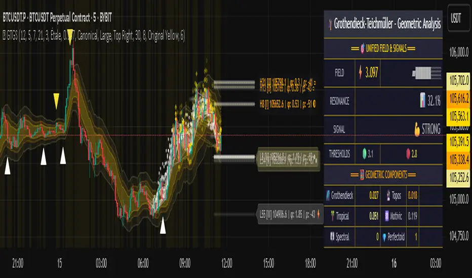
Volume Block Order AnalyzerCore Concept
The Volume Block Order Analyzer is a sophisticated Pine Script strategy designed to detect and analyze institutional money flow through large block trades. It identifies unusually high volume candles and evaluates their directional bias to provide clear visual signals of potential market movements.
How It Works: The Mathematical Model
1. Volume Anomaly Detection
The strategy first identifies "block trades" using a statistical approach:
```
avgVolume = ta.sma(volume, lookbackPeriod)
isHighVolume = volume > avgVolume * volumeThreshold
```
This means a candle must have volume exceeding the recent average by a user-defined multiplier (default 2.0x) to be considered a significant block trade.
2. Directional Impact Calculation
For each block trade identified, its price action determines direction:
- Bullish candle (close > open): Positive impact
- Bearish candle (close < open): Negative impact
The magnitude of impact is proportional to the volume size:
```
volumeWeight = volume / avgVolume // How many times larger than average
blockImpact = (isBullish ? 1.0 : -1.0) * (volumeWeight / 10)
```
This creates a normalized impact score typically ranging from -1.0 to 1.0, scaled by dividing by 10 to prevent excessive values.
3. Cumulative Impact with Time Decay
The key innovation is the cumulative impact calculation with decay:
```
cumulativeImpact := cumulativeImpact * impactDecay + blockImpact
```
This mathematical model has important properties:
- Recent block trades have stronger influence than older ones
- Impact gradually "fades" at rate determined by decay factor (default 0.95)
- Sustained directional pressure accumulates over time
- Opposing pressure gradually counteracts previous momentum
Trading Logic
Signal Generation
The strategy generates trading signals based on momentum shifts in institutional order flow:
1. Long Entry Signal: When cumulative impact crosses from negative to positive
```
if ta.crossover(cumulativeImpact, 0)
strategy.entry("Long", strategy.long)
```
*Logic: Institutional buying pressure has overcome selling pressure, indicating potential upward movement*
2. Short Entry Signal: When cumulative impact crosses from positive to negative
```
if ta.crossunder(cumulativeImpact, 0)
strategy.entry("Short", strategy.short)
```
*Logic: Institutional selling pressure has overcome buying pressure, indicating potential downward movement*
3. Exit Logic: Positions are closed when the cumulative impact moves against the position
```
if cumulativeImpact < 0
strategy.close("Long")
```
*Logic: The original signal is no longer valid as institutional flow has reversed*
Visual Interpretation System
The strategy employs multiple visualization techniques:
1. Color Gradient Bar System:
- Deep green: Strong buying pressure (impact > 0.5)
- Light green: Moderate buying pressure (0.1 < impact ≤ 0.5)
- Yellow-green: Mild buying pressure (0 < impact ≤ 0.1)
- Yellow: Neutral (impact = 0)
- Yellow-orange: Mild selling pressure (-0.1 < impact ≤ 0)
- Orange: Moderate selling pressure (-0.5 < impact ≤ -0.1)
- Red: Strong selling pressure (impact ≤ -0.5)
2. Dynamic Impact Line:
- Plots the cumulative impact as a line
- Line color shifts with impact value
- Line movement shows momentum and trend strength
3. Block Trade Labels:
- Marks significant block trades directly on the chart
- Shows direction and volume amount
- Helps identify key moments of institutional activity
4. Information Dashboard:
- Current impact value and signal direction
- Average volume benchmark
- Count of significant block trades
- Min/Max impact range
Benefits and Use Cases
This strategy provides several advantages:
1. Institutional Flow Detection: Identifies where large players are positioning themselves
2. Early Trend Identification: Often detects institutional accumulation/distribution before major price movements
3. Market Context Enhancement: Provides deeper insight than simple price action alone
4. Objective Decision Framework: Quantifies what might otherwise be subjective observations
5. Adaptive to Market Conditions: Works across different timeframes and instruments by using relative volume rather than absolute thresholds
Customization Options
The strategy allows users to fine-tune its behavior:
- Volume Threshold: How unusual a volume spike must be to qualify
- Lookback Period: How far back to measure average volume
- Impact Decay Factor: How quickly older trades lose influence
- Visual Settings: Labels and line width customization
This sophisticated yet intuitive strategy provides traders with a window into institutional activity, helping identify potential trend changes before they become obvious in price action alone.
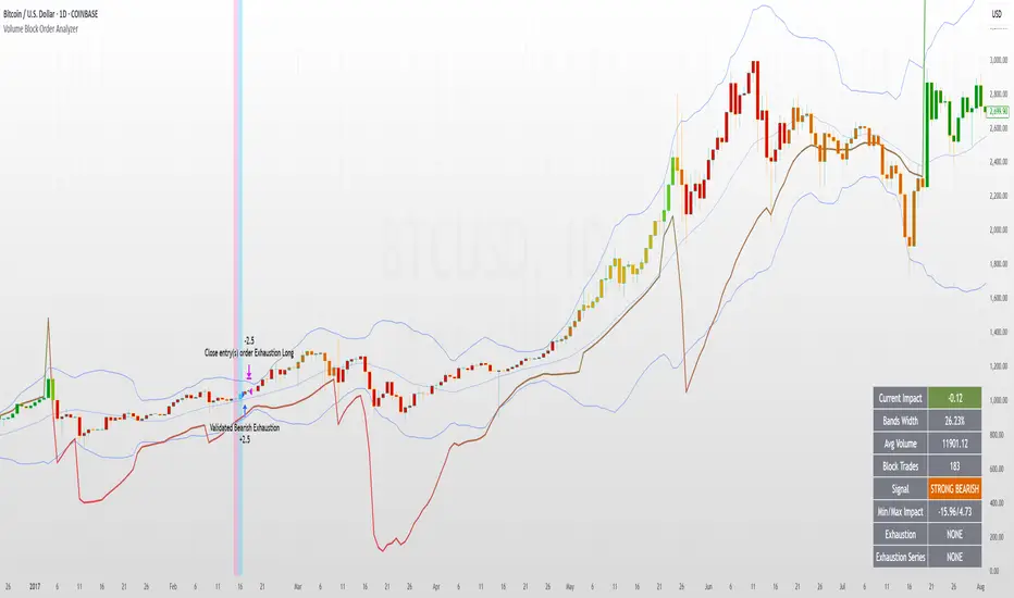
S&P 500 Sector StrengthsThe "S&P 500 Sector Strengths" indicator is a sophisticated tool designed to provide traders and investors with a comprehensive view of the relative performance of various sectors within the S&P 500 index. This indicator utilizes the True Strength Index (TSI) to measure and compare the strength of different sectors, offering valuable insights into market trends and sector rotations.
At its core, the indicator calculates the TSI for each sector using price data obtained through the request.security() function. The TSI, a momentum oscillator, is computed using a user-defined smoothing period, allowing for customization based on individual preferences and trading styles. The resulting TSI values for each sector are then plotted on the chart, creating a visual representation of sector strengths.
To use this indicator effectively, traders should focus on comparing the movements of different sector lines. Sectors with lines moving higher are showing increasing strength, while those with descending lines are exhibiting weakness. This comparative analysis can help identify potential investment opportunities and sector rotations. Additionally, when multiple sector lines move in tandem, it may signal a broader market trend.
The indicator includes dashed lines at 0.5 and -0.5, serving as reference points for overbought and oversold conditions. Sectors with TSI values above 0.5 might be considered overbought, suggesting caution, while those below -0.5 could be viewed as oversold, potentially indicating buying opportunities.
One of the key advantages of this indicator is its flexibility. Users can toggle the visibility of individual sectors and customize their colors, allowing for a tailored analysis experience. This feature is particularly useful when focusing on specific sectors or reducing chart clutter for clearer visualization.
The indicator's ability to provide a comprehensive overview of all major S&P 500 sectors in a single chart is a significant benefit. This consolidated view enables quick comparisons and helps in identifying relative strengths and weaknesses across sectors. Such insights can be invaluable for portfolio allocation decisions and in spotting emerging market trends.
Moreover, the dynamic legend feature enhances the indicator's usability. It automatically updates to display only the visible sectors, improving chart readability and interpretation.
By leveraging this indicator, market participants can gain a deeper understanding of sector dynamics within the S&P 500. This enhanced perspective can lead to more informed decision-making in sector allocation strategies and individual stock selection. The indicator's ability to potentially detect early trends by comparing sector strengths adds another layer of value, allowing users to position themselves ahead of broader market movements.
In conclusion, the "S&P 500 Sector Strengths" indicator is a powerful tool that combines technical analysis with sector comparison. Its user-friendly interface, customizable features, and comprehensive sector coverage make it an valuable asset for traders and investors seeking to navigate the complexities of the S&P 500 market with greater confidence and insight.
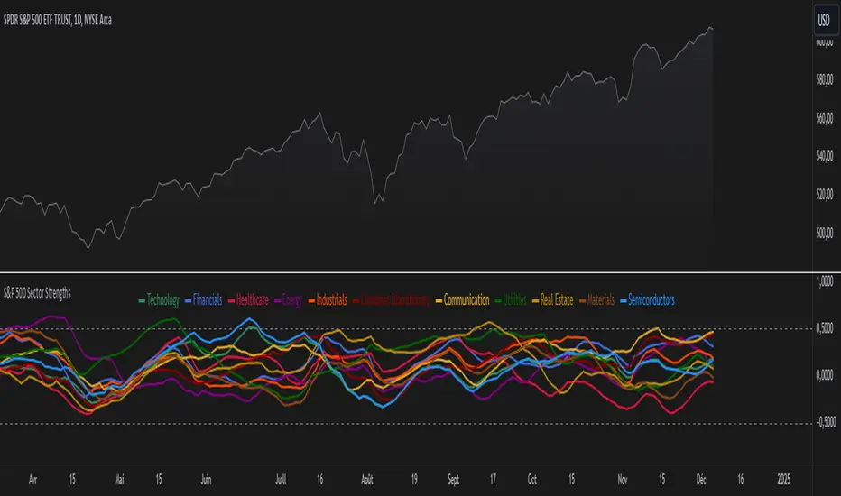
FTMO Rules MonitorFTMO Rules Monitor: Stay on Track with Your FTMO Challenge Goals
TLDR; You can test with this template whether your strategy for one asset would pass the FTMO challenges step 1 then step 2, then with real money conditions.
Passing a prop firm challenge is ... challenging.
I believe a toolkit allowing to test in minutes whether a strategy would have passed a prop firm challenge in the past could be very powerful.
The FTMO Rules Monitor is designed to help you stay within FTMO’s strict risk management guidelines directly on your chart. Whether you’re aiming for the $10,000 or the $200,000 account challenge, this tool provides real-time tracking of your performance against FTMO’s rules to ensure you don’t accidentally breach any limits.
NOTES
The connected indicator for this post doesn't matter.
It's just a dummy double supertrends (see below)
The strategy results for this script post does not matter as I'm posting a FTMO rules template on which you can connect any indicator/strategy.
//@version=5
indicator("Supertrends", overlay=true)
// Supertrend 1 Parameters
var string ST1 = "Supertrend 1 Settings"
st1_atrPeriod = input.int(10, "ATR Period", minval=1, maxval=50, group=ST1)
st1_factor = input.float(2, "Factor", minval=0.5, maxval=10, step=0.5, group=ST1)
// Supertrend 2 Parameters
var string ST2 = "Supertrend 2 Settings"
st2_atrPeriod = input.int(14, "ATR Period", minval=1, maxval=50, group=ST2)
st2_factor = input.float(3, "Factor", minval=0.5, maxval=10, step=0.5, group=ST2)
// Calculate Supertrends
= ta.supertrend(st1_factor, st1_atrPeriod)
= ta.supertrend(st2_factor, st2_atrPeriod)
// Entry conditions
longCondition = direction1 == -1 and direction2 == -1 and direction1 == 1
shortCondition = direction1 == 1 and direction2 == 1 and direction1 == -1
// Optional: Plot Supertrends
plot(supertrend1, "Supertrend 1", color = direction1 == -1 ? color.green : color.red, linewidth=3)
plot(supertrend2, "Supertrend 2", color = direction2 == -1 ? color.lime : color.maroon, linewidth=3)
plotshape(series=longCondition, location=location.belowbar, color=color.green, style=shape.triangleup, title="Long")
plotshape(series=shortCondition, location=location.abovebar, color=color.red, style=shape.triangledown, title="Short")
signal = longCondition ? 1 : shortCondition ? -1 : na
plot(signal, "Signal", display = display.data_window)
To connect your indicator to this FTMO rules monitor template, please update it as follow
Create a signal variable to store 1 for the long/buy signal or -1 for the short/sell signal
Plot it in the display.data_window panel so that it doesn't clutter your chart
signal = longCondition ? 1 : shortCondition ? -1 : na
plot(signal, "Signal", display = display.data_window)
In the FTMO Rules Monitor template, I'm capturing this external signal with this input.source variable
entry_connector = input.source(close, "Entry Connector", group="Entry Connector")
longCondition = entry_connector == 1
shortCondition = entry_connector == -1
🔶 USAGE
This indicator displays essential FTMO Challenge rules and tracks your progress toward meeting each one. Here’s what’s monitored:
Max Daily Loss
• 10k Account: $500
• 25k Account: $1,250
• 50k Account: $2,500
• 100k Account: $5,000
• 200k Account: $10,000
Max Total Loss
• 10k Account: $1,000
• 25k Account: $2,500
• 50k Account: $5,000
• 100k Account: $10,000
• 200k Account: $20,000
Profit Target
• 10k Account: $1,000
• 25k Account: $2,500
• 50k Account: $5,000
• 100k Account: $10,000
• 200k Account: $20,000
Minimum Trading Days: 4 consecutive days for all account sizes
🔹 Key Features
1. Real-Time Compliance Check
The FTMO Rules Monitor keeps track of your daily and total losses, profit targets, and trading days. Each metric updates in real-time, giving you peace of mind that you’re within FTMO’s rules.
2. Color-Coded Visual Feedback
Each rule’s status is shown clearly with a ✓ for compliance or ✗ if the limit is breached. When a rule is broken, the indicator highlights it in red, so there’s no confusion.
3. Completion Notification
Once all FTMO requirements are met, the indicator closes all open positions and displays a celebratory message on your chart, letting you know you’ve successfully completed the challenge.
4. Easy-to-Read Table
A table on your chart provides an overview of each rule, your target, current performance, and whether you’re meeting each goal. The table adjusts its color scheme based on your chart settings for optimal visibility.
5. Dynamic Position Sizing
Integrated ATR-based position sizing helps you manage risk and avoid large drawdowns, ensuring each trade aligns with FTMO’s risk management principles.
Daveatt

Trading IQ - ICT LibraryLibrary "ICTlibrary"
Used to calculate various ICT related price levels and strategies. An ongoing project.
Hello Coders!
This library is meant for sourcing ICT related concepts. While some functions might generate more output than you require, you can specify "Lite Mode" as "true" in applicable functions to slim down necessary inputs.
isLastBar(userTF)
Identifies the last bar on the chart before a timeframe change
Parameters:
userTF (simple int) : the timeframe you wish to calculate the last bar for, must be converted to integer using 'timeframe.in_seconds()'
Returns: bool true if bar on chart is last bar of higher TF, dalse if bar on chart is not last bar of higher TF
necessaryData(atrTF)
returns necessaryData UDT for historical data access
Parameters:
atrTF (float) : user-selected timeframe ATR value.
Returns: logZ. log return Z score, used for calculating order blocks.
method gradBoxes(gradientBoxes, idColor, timeStart, bottom, top, rightCoordinate)
creates neon like effect for box drawings
Namespace types: array
Parameters:
gradientBoxes (array) : an array.new() to store the gradient boxes
idColor (color)
timeStart (int) : left point of box
bottom (float) : bottom of box price point
top (float) : top of box price point
rightCoordinate (int) : right point of box
Returns: void
checkIfTraded(tradeName)
checks if recent trade is of specific name
Parameters:
tradeName (string)
Returns: bool true if recent trade id matches target name, false otherwise
checkIfClosed(tradeName)
checks if recent closed trade is of specific name
Parameters:
tradeName (string)
Returns: bool true if recent closed trade id matches target name, false otherwise
IQZZ(atrMult, finalTF)
custom ZZ to quickly determine market direction.
Parameters:
atrMult (float) : an atr multiplier used to determine the required price move for a ZZ direction change
finalTF (string) : the timeframe used for the atr calcuation
Returns: dir market direction. Up => 1, down => -1
method drawBos(id, startPoint, getKeyPointTime, getKeyPointPrice, col, showBOS, isUp)
calculates and draws Break Of Structure
Namespace types: array
Parameters:
id (array)
startPoint (chart.point)
getKeyPointTime (int) : the actual time of startPoint, simplystartPoint.time
getKeyPointPrice (float) : the actual time of startPoint, simplystartPoint.price
col (color) : color of the BoS line / label
showBOS (bool) : whether to show label/line. This function still calculates internally for other ICT related concepts even if not drawn.
isUp (bool) : whether BoS happened during price increase or price decrease.
Returns: void
method drawMSS(id, startPoint, getKeyPointTime, getKeyPointPrice, col, showMSS, isUp, upRejections, dnRejections, highArr, lowArr, timeArr, closeArr, openArr, atrTFarr, upRejectionsPrices, dnRejectionsPrices)
calculates and draws Market Structure Shift. This data is also used to calculate Rejection Blocks.
Namespace types: array
Parameters:
id (array)
startPoint (chart.point)
getKeyPointTime (int) : the actual time of startPoint, simplystartPoint.time
getKeyPointPrice (float) : the actual time of startPoint, simplystartPoint.price
col (color) : color of the MSS line / label
showMSS (bool) : whether to show label/line. This function still calculates internally for other ICT related concepts even if not drawn.
isUp (bool) : whether MSS happened during price increase or price decrease.
upRejections (array)
dnRejections (array)
highArr (array) : array containing historical highs, should be taken from the UDT "necessaryData" defined above
lowArr (array) : array containing historical lows, should be taken from the UDT "necessaryData" defined above
timeArr (array) : array containing historical times, should be taken from the UDT "necessaryData" defined above
closeArr (array) : array containing historical closes, should be taken from the UDT "necessaryData" defined above
openArr (array) : array containing historical opens, should be taken from the UDT "necessaryData" defined above
atrTFarr (array) : array containing historical atr values (of user-selected TF), should be taken from the UDT "necessaryData" defined above
upRejectionsPrices (array) : array containing up rejections prices. Is sorted and used to determine selective looping for invalidations.
dnRejectionsPrices (array) : array containing down rejections prices. Is sorted and used to determine selective looping for invalidations.
Returns: void
method getTime(id, compare, timeArr)
gets time of inputted price (compare) in an array of data
this is useful when the user-selected timeframe for ICT concepts is greater than the chart's timeframe
Namespace types: array
Parameters:
id (array) : the array of data to search through, to find which index has the same value as "compare"
compare (float) : the target data point to find in the array
timeArr (array) : array of historical times
Returns: the time that the data point in the array was recorded
method OB(id, highArr, signArr, lowArr, timeArr, sign)
store bullish orderblock data
Namespace types: array
Parameters:
id (array)
highArr (array) : array of historical highs
signArr (array) : array of historical price direction "math.sign(close - open)"
lowArr (array) : array of historical lows
timeArr (array) : array of historical times
sign (int) : orderblock direction, -1 => bullish, 1 => bearish
Returns: void
OTEstrat(OTEstart, future, closeArr, highArr, lowArr, timeArr, longOTEPT, longOTESL, longOTElevel, shortOTEPT, shortOTESL, shortOTElevel, structureDirection, oteLongs, atrTF, oteShorts)
executes the OTE strategy
Parameters:
OTEstart (chart.point)
future (int) : future time point for drawings
closeArr (array) : array of historical closes
highArr (array) : array of historical highs
lowArr (array) : array of historical lows
timeArr (array) : array of historical times
longOTEPT (string) : user-selected long OTE profit target, please create an input.string() for this using the example below
longOTESL (int) : user-selected long OTE stop loss, please create an input.string() for this using the example below
longOTElevel (float) : long entry price of selected retracement ratio for OTE
shortOTEPT (string) : user-selected short OTE profit target, please create an input.string() for this using the example below
shortOTESL (int) : user-selected short OTE stop loss, please create an input.string() for this using the example below
shortOTElevel (float) : short entry price of selected retracement ratio for OTE
structureDirection (string) : current market structure direction, this should be "Up" or "Down". This is used to cancel pending orders if market structure changes
oteLongs (bool) : input.bool() for whether OTE longs can be executed
atrTF (float) : atr of the user-seleceted TF
oteShorts (bool) : input.bool() for whether OTE shorts can be executed
@exampleInputs
oteLongs = input.bool(defval = false, title = "OTE Longs", group = "Optimal Trade Entry")
longOTElevel = input.float(defval = 0.79, title = "Long Entry Retracement Level", options = , group = "Optimal Trade Entry")
longOTEPT = input.string(defval = "-0.5", title = "Long TP", options = , group = "Optimal Trade Entry")
longOTESL = input.int(defval = 0, title = "How Many Ticks Below Swing Low For Stop Loss", group = "Optimal Trade Entry")
oteShorts = input.bool(defval = false, title = "OTE Shorts", group = "Optimal Trade Entry")
shortOTElevel = input.float(defval = 0.79, title = "Short Entry Retracement Level", options = , group = "Optimal Trade Entry")
shortOTEPT = input.string(defval = "-0.5", title = "Short TP", options = , group = "Optimal Trade Entry")
shortOTESL = input.int(defval = 0, title = "How Many Ticks Above Swing Low For Stop Loss", group = "Optimal Trade Entry")
Returns: void (0)
displacement(logZ, atrTFreg, highArr, timeArr, lowArr, upDispShow, dnDispShow, masterCoords, labelLevels, dispUpcol, rightCoordinate, dispDncol, noBorders)
calculates and draws dispacements
Parameters:
logZ (float) : log return of current price, used to determine a "significant price move" for a displacement
atrTFreg (float) : atr of user-seleceted timeframe
highArr (array) : array of historical highs
timeArr (array) : array of historical times
lowArr (array) : array of historical lows
upDispShow (int) : amount of historical upside displacements to show
dnDispShow (int) : amount of historical downside displacements to show
masterCoords (map) : a map to push the most recent displacement prices into, useful for having key levels in one data structure
labelLevels (string) : used to determine label placement for the displacement, can be inside box, outside box, or none, example below
dispUpcol (color) : upside displacement color
rightCoordinate (int) : future time for displacement drawing, best is "last_bar_time"
dispDncol (color) : downside displacement color
noBorders (bool) : input.bool() to remove box borders, example below
@exampleInputs
labelLevels = input.string(defval = "Inside" , title = "Box Label Placement", options = )
noBorders = input.bool(defval = false, title = "No Borders On Levels")
Returns: void
method getStrongLow(id, startIndex, timeArr, lowArr, strongLowPoints)
unshift strong low data to array id
Namespace types: array
Parameters:
id (array)
startIndex (int) : the starting index for the timeArr array of the UDT "necessaryData".
this point should start from at least 1 pivot prior to find the low before an upside BoS
timeArr (array) : array of historical times
lowArr (array) : array of historical lows
strongLowPoints (array) : array of strong low prices. Used to retrieve highest strong low price and see if need for
removal of invalidated strong lows
Returns: void
method getStrongHigh(id, startIndex, timeArr, highArr, strongHighPoints)
unshift strong high data to array id
Namespace types: array
Parameters:
id (array)
startIndex (int) : the starting index for the timeArr array of the UDT "necessaryData".
this point should start from at least 1 pivot prior to find the high before a downside BoS
timeArr (array) : array of historical times
highArr (array) : array of historical highs
strongHighPoints (array)
Returns: void
equalLevels(highArr, lowArr, timeArr, rightCoordinate, equalHighsCol, equalLowsCol, liteMode)
used to calculate recent equal highs or equal lows
Parameters:
highArr (array) : array of historical highs
lowArr (array) : array of historical lows
timeArr (array) : array of historical times
rightCoordinate (int) : a future time (right for boxes, x2 for lines)
equalHighsCol (color) : user-selected color for equal highs drawings
equalLowsCol (color) : user-selected color for equal lows drawings
liteMode (bool) : optional for a lite mode version of an ICT strategy. For more control over drawings leave as "True", "False" will apply neon effects
Returns: void
quickTime(timeString)
used to quickly determine if a user-inputted time range is currently active in NYT time
Parameters:
timeString (string) : a time range
Returns: true if session is active, false if session is inactive
macros(showMacros, noBorders)
used to calculate and draw session macros
Parameters:
showMacros (bool) : an input.bool() or simple bool to determine whether to activate the function
noBorders (bool) : an input.bool() to determine whether the box anchored to the session should have borders
Returns: void
po3(tf, left, right, show)
use to calculate HTF po3 candle
@tip only call this function on "barstate.islast"
Parameters:
tf (simple string)
left (int) : the left point of the candle, calculated as bar_index + left,
right (int) : :the right point of the candle, calculated as bar_index + right,
show (bool) : input.bool() whether to show the po3 candle or not
Returns: void
silverBullet(silverBulletStratLong, silverBulletStratShort, future, userTF, H, L, H2, L2, noBorders, silverBulletLongTP, historicalPoints, historicalData, silverBulletLongSL, silverBulletShortTP, silverBulletShortSL)
used to execute the Silver Bullet Strategy
Parameters:
silverBulletStratLong (simple bool)
silverBulletStratShort (simple bool)
future (int) : a future time, used for drawings, example "last_bar_time"
userTF (simple int)
H (float) : the high price of the user-selected TF
L (float) : the low price of the user-selected TF
H2 (float) : the high price of the user-selected TF
L2 (float) : the low price of the user-selected TF
noBorders (bool) : an input.bool() used to remove the borders from box drawings
silverBulletLongTP (series silverBulletLevels)
historicalPoints (array)
historicalData (necessaryData)
silverBulletLongSL (series silverBulletLevels)
silverBulletShortTP (series silverBulletLevels)
silverBulletShortSL (series silverBulletLevels)
Returns: void
method invalidFVGcheck(FVGarr, upFVGpricesSorted, dnFVGpricesSorted)
check if existing FVGs are still valid
Namespace types: array
Parameters:
FVGarr (array)
upFVGpricesSorted (array) : an array of bullish FVG prices, used to selective search through FVG array to remove invalidated levels
dnFVGpricesSorted (array) : an array of bearish FVG prices, used to selective search through FVG array to remove invalidated levels
Returns: void (0)
method drawFVG(counter, FVGshow, FVGname, FVGcol, data, masterCoords, labelLevels, borderTransp, liteMode, rightCoordinate)
draws FVGs on last bar
Namespace types: map
Parameters:
counter (map) : a counter, as map, keeping count of the number of FVGs drawn, makes sure that there aren't more FVGs drawn
than int FVGshow
FVGshow (int) : the number of FVGs to show. There should be a bullish FVG show and bearish FVG show. This function "drawFVG" is used separately
for bearish FVG and bullish FVG.
FVGname (string) : the name of the FVG, "FVG Up" or "FVG Down"
FVGcol (color) : desired FVG color
data (FVG)
masterCoords (map) : a map containing the names and price points of key levels. Used to define price ranges.
labelLevels (string) : an input.string with options "Inside", "Outside", "Remove". Determines whether FVG labels should be inside box, outside,
or na.
borderTransp (int)
liteMode (bool)
rightCoordinate (int) : the right coordinate of any drawings. Must be a time point.
Returns: void
invalidBlockCheck(bullishOBbox, bearishOBbox, userTF)
check if existing order blocks are still valid
Parameters:
bullishOBbox (array) : an array declared using the UDT orderBlock that contains bullish order block related data
bearishOBbox (array) : an array declared using the UDT orderBlock that contains bearish order block related data
userTF (simple int)
Returns: void (0)
method lastBarRejections(id, rejectionColor, idShow, rejectionString, labelLevels, borderTransp, liteMode, rightCoordinate, masterCoords)
draws rejectionBlocks on last bar
Namespace types: array
Parameters:
id (array) : the array, an array of rejection block data declared using the UDT rejection block
rejectionColor (color) : the desired color of the rejection box
idShow (int)
rejectionString (string) : the desired name of the rejection blocks
labelLevels (string) : an input.string() to determine if labels for the block should be inside the box, outside, or none.
borderTransp (int)
liteMode (bool) : an input.bool(). True = neon effect, false = no neon.
rightCoordinate (int) : atime for the right coordinate of the box
masterCoords (map) : a map that stores the price of key levels and assigns them a name, used to determine price ranges
Returns: void
method OBdraw(id, OBshow, BBshow, OBcol, BBcol, bullishString, bearishString, isBullish, labelLevels, borderTransp, liteMode, rightCoordinate, masterCoords)
draws orderblocks and breaker blocks for data stored in UDT array()
Namespace types: array
Parameters:
id (array) : the array, an array of order block data declared using the UDT orderblock
OBshow (int) : the number of order blocks to show
BBshow (int) : the number of breaker blocks to show
OBcol (color) : color of order blocks
BBcol (color) : color of breaker blocks
bullishString (string) : the title of bullish blocks, which is a regular bullish orderblock or a bearish orderblock that's converted to breakerblock
bearishString (string) : the title of bearish blocks, which is a regular bearish orderblock or a bullish orderblock that's converted to breakerblock
isBullish (bool) : whether the array contains bullish orderblocks or bearish orderblocks. If bullish orderblocks,
the array will naturally contain bearish BB, and if bearish OB, the array will naturally contain bullish BB
labelLevels (string) : an input.string() to determine if labels for the block should be inside the box, outside, or none.
borderTransp (int)
liteMode (bool) : an input.bool(). True = neon effect, false = no neon.
rightCoordinate (int) : atime for the right coordinate of the box
masterCoords (map) : a map that stores the price of key levels and assigns them a name, used to determine price ranges
Returns: void
FVG
UDT for FVG calcualtions
Fields:
H (series float) : high price of user-selected timeframe
L (series float) : low price of user-selected timeframe
direction (series string) : FVG direction => "Up" or "Down"
T (series int) : => time of bar on user-selected timeframe where FVG was created
fvgLabel (series label) : optional label for FVG
fvgLineTop (series line) : optional line for top of FVG
fvgLineBot (series line) : optional line for bottom of FVG
fvgBox (series box) : optional box for FVG
labelLine
quickly pair a line and label together as UDT
Fields:
lin (series line) : Line you wish to pair with label
lab (series label) : Label you wish to pair with line
orderBlock
UDT for order block calculations
Fields:
orderBlockData (array) : array containing order block x and y points
orderBlockBox (series box) : optional order block box
vioCount (series int) : = 0 violation count of the order block. 0 = Order Block, 1 = Breaker Block
traded (series bool)
status (series string) : = "OB" status == "OB" => Level is order block. status == "BB" => Level is breaker block.
orderBlockLab (series label) : options label for the order block / breaker block.
strongPoints
UDT for strong highs and strong lows
Fields:
price (series float) : price of the strong high or strong low
timeAtprice (series int) : time of the strong high or strong low
strongPointLabel (series label) : optional label for strong point
strongPointLine (series line) : optional line for strong point
overlayLine (series line) : optional lines for strong point to enhance visibility
overlayLine2 (series line) : optional lines for strong point to enhance visibility
displacement
UDT for dispacements
Fields:
highPrice (series float) : high price of displacement
lowPrice (series float) : low price of displacement
timeAtPrice (series int) : time of bar where displacement occurred
displacementBox (series box) : optional box to draw displacement
displacementLab (series label) : optional label for displacement
po3data
UDT for po3 calculations
Fields:
dHigh (series float) : higher timeframe high price
dLow (series float) : higher timeframe low price
dOpen (series float) : higher timeframe open price
dClose (series float) : higher timeframe close price
po3box (series box) : box to draw po3 candle body
po3line (array) : line array to draw po3 wicks
po3Labels (array) : label array to label price points of po3 candle
macros
UDT for session macros
Fields:
sessions (array) : Array of sessions, you can populate this array using the "quickTime" function located above "export macros".
prices (matrix) : Matrix of session data -> open, high, low, close, time
sessionTimes (array) : Array of session names. Pairs with array sessions.
sessionLines (matrix) : Optional array for sesion drawings.
OTEtimes
UDT for data storage and drawings associated with OTE strategy
Fields:
upTimes (array) : time of highest point before trade is taken
dnTimes (array) : time of lowest point before trade is taken
tpLineLong (series line) : line to mark tp level long
tpLabelLong (series label) : label to mark tp level long
slLineLong (series line) : line to mark sl level long
slLabelLong (series label) : label to mark sl level long
tpLineShort (series line) : line to mark tp level short
tpLabelShort (series label) : label to mark tp level short
slLineShort (series line) : line to mark sl level short
slLabelShort (series label) : label to mark sl level short
sweeps
UDT for data storage and drawings associated with liquidity sweeps
Fields:
upSweeps (matrix) : matrix containing liquidity sweep price points and time points for up sweeps
dnSweeps (matrix) : matrix containing liquidity sweep price points and time points for down sweeps
upSweepDrawings (array) : optional up sweep box array. Pair the size of this array with the rows or columns,
dnSweepDrawings (array) : optional up sweep box array. Pair the size of this array with the rows or columns,
raidExitDrawings
UDT for drawings associated with the Liquidity Raid Strategy
Fields:
tpLine (series line) : tp line for the liquidity raid entry
tpLabel (series label) : tp label for the liquidity raid entry
slLine (series line) : sl line for the liquidity raid entry
slLabel (series label) : sl label for the liquidity raid entry
m2022
UDT for data storage and drawings associated with the Model 2022 Strategy
Fields:
mTime (series int) : time of the FVG where entry limit order is placed
mIndex (series int) : array index of FVG where entry limit order is placed. This requires an array of FVG data, which is defined above.
mEntryDistance (series float) : the distance of the FVG to the 50% range. M2022 looks for the fvg closest to 50% mark of range.
mEntry (series float) : the entry price for the most eligible fvg
fvgHigh (series float) : the high point of the eligible fvg
fvgLow (series float) : the low point of the eligible fvg
longFVGentryBox (series box) : long FVG box, used to draw the eligible FVG
shortFVGentryBox (series box) : short FVG box, used to draw the eligible FVG
line50P (series line) : line used to mark 50% of the range
line100P (series line) : line used to mark 100% (top) of the range
line0P (series line) : line used to mark 0% (bottom) of the range
label50P (series label) : label used to mark 50% of the range
label100P (series label) : label used to mark 100% (top) of the range
label0P (series label) : label used to mark 0% (bottom) of the range
sweepData (array)
silverBullet
UDT for data storage and drawings associated with the Silver Bullet Strategy
Fields:
session (series bool)
sessionStr (series string) : name of the session for silver bullet
sessionBias (series string)
sessionHigh (series float) : = high high of session // use math.max(silverBullet.sessionHigh, high)
sessionLow (series float) : = low low of session // use math.min(silverBullet.sessionLow, low)
sessionFVG (series float) : if applicable, the FVG created during the session
sessionFVGdraw (series box) : if applicable, draw the FVG created during the session
traded (series bool)
tp (series float) : tp of trade entered at the session FVG
sl (series float) : sl of trade entered at the session FVG
sessionDraw (series box) : optional draw session with box
sessionDrawLabel (series label) : optional label session with label
silverBulletDrawings
UDT for trade exit drawings associated with the Silver Bullet Strategy
Fields:
tpLine (series line) : tp line drawing for strategy
tpLabel (series label) : tp label drawing for strategy
slLine (series line) : sl line drawing for strategy
slLabel (series label) : sl label drawing for strategy
unicornModel
UDT for data storage and drawings associated with the Unicorn Model Strategy
Fields:
hPoint (chart.point)
hPoint2 (chart.point)
hPoint3 (chart.point)
breakerBlock (series box) : used to draw the breaker block required for the Unicorn Model
FVG (series box) : used to draw the FVG required for the Unicorn model
topBlock (series float) : price of top of breaker block, can be used to detail trade entry
botBlock (series float) : price of bottom of breaker block, can be used to detail trade entry
startBlock (series int) : start time of the breaker block, used to set the "left = " param for the box
includes (array) : used to store the time of the breaker block, or FVG, or the chart point sequence that setup the Unicorn Model.
entry (series float) : // eligible entry price, for longs"math.max(topBlock, FVG.get_top())",
tpLine (series line) : optional line to mark PT
tpLabel (series label) : optional label to mark PT
slLine (series line) : optional line to mark SL
slLabel (series label) : optional label to mark SL
rejectionBlocks
UDT for data storage and drawings associated with rejection blocks
Fields:
rejectionPoint (chart.point)
bodyPrice (series float) : candle body price closest to the rejection point, for "Up" rejections => math.max(open, close),
rejectionBox (series box) : optional box drawing of the rejection block
rejectionLabel (series label) : optional label for the rejection block
equalLevelsDraw
UDT for data storage and drawings associated with equal highs / equal lows
Fields:
connector (series line) : single line placed at the first high or low, y = avgerage of distinguished equal highs/lows
connectorLab (series label) : optional label to be placed at the highs or lows
levels (array) : array containing the equal highs or lows prices
times (array) : array containing the equal highs or lows individual times
startTime (series int) : the time of the first high or low that forms a sequence of equal highs or lows
radiate (array) : options label to "radiate" the label in connector lab. Can be used for anything
necessaryData
UDT for data storage of historical price points.
Fields:
highArr (array) : array containing historical high points
lowArr (array) : array containing historical low points
timeArr (array) : array containing historical time points
logArr (array) : array containing historical log returns
signArr (array) : array containing historical price directions
closeArr (array) : array containing historical close points
binaryTimeArr (array) : array containing historical time points, uses "push" instead of "unshift" to allow for binary search
binaryCloseArr (array) : array containing historical close points, uses "push" instead of "unshift" to allow the correct
binaryOpenArr (array) : array containing historical optn points, uses "push" instead of "unshift" to allow the correct
atrTFarr (array) : array containing historical user-selected TF atr points
openArr (array) : array containing historical open points

MA rate of changeThis indicator uses moving averages to determine trends. For those who trade using a trend-following strategy, it's not possible to use the slope of the moving average line as an indicator of trend judgment if it's expressed as an angle. This is because the angle changes depending on the adjustments made to the vertical price scale and horizontal time scale of the chart.
Therefore, instead of using the angle, I decided to use the rate of change in price as an alternative indicator.
The relationship between the rate of change of the moving average and the angle of the moving average line is as follows:
- When the value is positive, the moving average line slopes upward.
- When the value is negative, the moving average line slopes downward.
- The larger the absolute value of the rate of change, the steeper the angle; the smaller the value, the gentler the slope.
The trend is determined using the rate of change instead of the angle, as follows:
- Uptrend: Rate of change > 0.5 (this value can be adjusted) ⇒ Display with a red background
- Downtrend: Rate of change < -0.5 (this value can be adjusted) ⇒ Display with a blue background
An example of a trade using this indicator is as follows:
- Enter the trade the day after the trend appears.
- Exit the trade the day after the trend ends.
このインジケーターは移動平均線を使ってトレンドを判断します。トレンドフォロー戦略でトレードする方はこのインジケーターの示す移動平均線の傾きを角度で表してトレンドの判定の指標とすることはできません。なぜなら、角度はチャートの縦軸の価格スケールや横軸の時間のスケールを調整することで変わってしまうからです。
そこで角度に代わる別の指標として価格の変化率を使うことにしました。
移動平均の変化率と、移動平均線の角度の関係は次の通りです。
- プラスの値の場合は移動平均線は右肩上がり
- マイナスの値の場合は移動平均線は右肩下がり
- 変化率の絶対値が大きいほど角度は急になり、小さいほど角度は緩やかになる
トレンドの判定は次のようにします。角度の代わりに変化率で判定します。
- 上昇トレンド : 変化率 > 0.5 (この値は調整可能) ⇒赤色の背景で表示
- 下降トレンド : 変化率 < -0.5 (この値は調整可能)⇒青色の背景で表示
このインジケーターを使ったトレードの例は次の通りです。
- トレンドが発生した翌日エントリー
- トレンドが終了した翌日エグジット

Fibonacci BandsDescription
This indicator dynamically calculates Fibonacci retracement levels based on the highest high and lowest low over a specified lookback period. The key Fibonacci levels (0.236, 0.382, 0.5, 0.618, and 0.786) are plotted on the chart, with shaded areas between these levels for visual guidance.
How it works
The script computes the highest high (hh) and the lowest low (ll) over the defined length.
It calculates the price range (delta) as the difference between the highest high and the lowest low.
Fibonacci levels are then determined using the formula: ℎℎ − (delta × Fibonacci ratio)
Each Fibonacci level is then plotted as a line with a specific color.
Key Features
Customizable Length: Users can adjust the lookback period to suit their trading strategy.
Multiple Fibonacci Levels: Includes common Fibonacci retracement levels, providing traders with a comprehensive view of potential support and resistance areas.
Visual Fillings: The script includes customizable shading between levels, which helps traders quickly identify key zones (like the "Golden Zone" between 0.5 and 0.618).
Unique Points
Fibonacci Focus: This script is specifically designed around Fibonacci retracement levels, which are popular among technical traders for identifying potential reversal points.
Dynamic Range Calculation: The use of the highest high and lowest low within a user-defined period offers a dynamic approach to adapting to changing market conditions.
How to use it
Adjust the length parameter (default is 60) to determine how many bars back the indicator will calculate the highest high and lowest low. A longer length may provide a broader perspective of price action, while a shorter length may react more quickly to recent price changes.
Observe the plotted Fibonacci levels: 0.236, 0.382, 0.5, 0.618, and 0.786. These levels often act as potential support and resistance points. Pay attention to how price interacts with these levels.
When the price approaches a Fibonacci level, consider it a potential reversal point. The filled areas between the Fibonacci levels indicate zones where price might consolidate or reverse. The "Golden Zone" (between 0.5 and 0.618) is particularly significant; many traders watch this area closely for potential entry points in an uptrend or exit points in a downtrend.
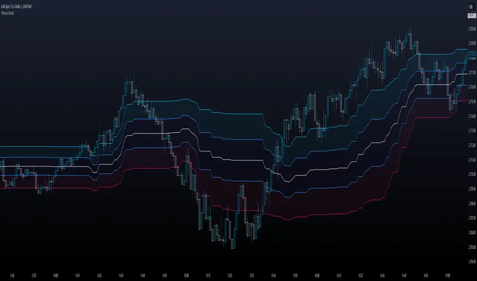
Correlation with AveragesThe "Correlation with Averages" indicator is designed to visualize and analyze the correlation between a selected asset's price and a base symbol's price, such as the S&P 500 (SPY). This indicator allows users to evaluate how closely an asset’s price movements align with those of the base symbol over various time periods, providing insights into market trends and potential portfolio adjustments.
Key Features:
Base Symbol and Correlation Period:
Users can specify the base symbol (default is SPY) and the period for correlation measurement (default is 252 trading days, approximating one year).
Correlation Calculation:
The indicator computes the correlation between the asset’s closing price and the base symbol’s closing price for the defined period.
Visualization:
The correlation value is plotted on the chart, with conditional background colors indicating the strength and direction of the correlation:
Red for negative correlation (below -0.5)
Green for positive correlation (above 0.5)
Yellow for neutral correlation (between -0.5 and 0.5)
Average Correlation Over Time:
Average correlations are calculated and displayed for various periods: one week, one month, one year, and five years.
A table on the chart provides dynamic updates of these average values with color-coded backgrounds to indicate correlation strength.
The Role of Correlation in Portfolio Management
Correlation is a crucial concept in portfolio management because it measures the degree to which two securities move in relation to each other. Understanding correlation helps investors construct diversified portfolios that balance risk and return. Here's why correlation is important:
Diversification:
By including assets with low or negative correlation in a portfolio, investors can reduce overall portfolio volatility and risk. For instance, if one asset is negatively correlated with another, when one performs poorly, the other may perform well, thus smoothing the overall returns.
Risk Management:
Correlation analysis helps in identifying the potential impact of one asset’s performance on the entire portfolio. Assets with high correlation can lead to concentrated risk, while those with low correlation offer better risk management.
Performance Analysis:
Correlation measures the degree to which asset returns move together. This can inform strategic decisions, such as whether to adjust positions based on expected market conditions.
Scientific References
Markowitz, H. M. (1952). "Portfolio Selection." Journal of Finance, 7(1), 77-91.
This foundational paper introduced Modern Portfolio Theory, highlighting the importance of diversification and correlation in reducing portfolio risk.
Jorion, P. (2007). Financial Risk Manager Handbook. Wiley.
This handbook provides an in-depth exploration of risk management techniques, including the use of correlation in portfolio management.
Elton, E. J., Gruber, M. J., Brown, S. J., & Goetzmann, W. N. (2014). Modern Portfolio Theory and Investment Analysis. Wiley.
This book elaborates on the concepts of correlation and diversification, offering practical insights into portfolio construction and risk management.
By utilizing the "Correlation with Averages" indicator, traders and portfolio managers can make informed decisions based on the relationship between asset prices and the base symbol, ultimately enhancing their investment strategies.
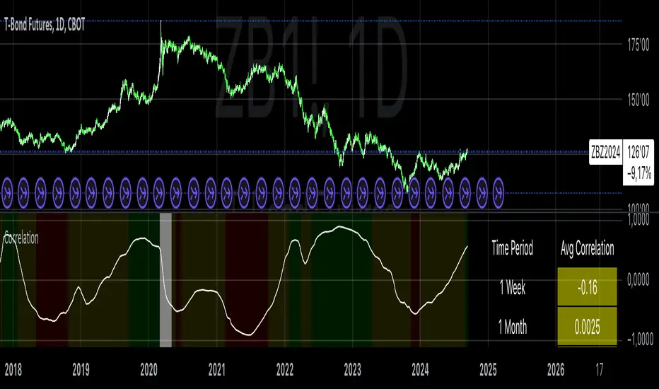
Bayesian Trend Indicator [ChartPrime]Bayesian Trend Indicator
Overview:
In probability theory and statistics, Bayes' theorem (alternatively Bayes' law or Bayes' rule), named after Thomas Bayes, describes the probability of an event, based on prior knowledge of conditions that might be related to the event.
The "Bayesian Trend Indicator" is a sophisticated technical analysis tool designed to assess the direction of price trends in financial markets. It combines the principles of Bayesian probability theory with moving average analysis to provide traders with a comprehensive understanding of market sentiment and potential trend reversals.
At its core, the indicator utilizes multiple moving averages, including the Exponential Moving Average (EMA), Simple Moving Average (SMA), Double Exponential Moving Average (DEMA), and Volume Weighted Moving Average (VWMA) . These moving averages are calculated based on user-defined parameters such as length and gap length, allowing traders to customize the indicator to suit their trading strategies and preferences.
The indicator begins by calculating the trend for both fast and slow moving averages using a Smoothed Gradient Signal Function. This function assigns a numerical value to each data point based on its relationship with historical data, indicating the strength and direction of the trend.
// Smoothed Gradient Signal Function
sig(float src, gap)=>
ta.ema(source >= src ? 1 :
source >= src ? 0.9 :
source >= src ? 0.8 :
source >= src ? 0.7 :
source >= src ? 0.6 :
source >= src ? 0.5 :
source >= src ? 0.4 :
source >= src ? 0.3 :
source >= src ? 0.2 :
source >= src ? 0.1 :
0, 4)
Next, the indicator calculates prior probabilities using the trend information from the slow moving averages and likelihood probabilities using the trend information from the fast moving averages . These probabilities represent the likelihood of an uptrend or downtrend based on historical data.
// Define prior probabilities using moving averages
prior_up = (ema_trend + sma_trend + dema_trend + vwma_trend) / 4
prior_down = 1 - prior_up
// Define likelihoods using faster moving averages
likelihood_up = (ema_trend_fast + sma_trend_fast + dema_trend_fast + vwma_trend_fast) / 4
likelihood_down = 1 - likelihood_up
Using Bayes' theorem , the indicator then combines the prior and likelihood probabilities to calculate posterior probabilities, which reflect the updated probability of an uptrend or downtrend given the current market conditions. These posterior probabilities serve as a key signal for traders, informing them about the prevailing market sentiment and potential trend reversals.
// Calculate posterior probabilities using Bayes' theorem
posterior_up = prior_up * likelihood_up
/
(prior_up * likelihood_up + prior_down * likelihood_down)
Key Features:
◆ The trend direction:
To visually represent the trend direction , the indicator colors the bars on the chart based on the posterior probabilities. Bars are colored green to indicate an uptrend when the posterior probability is greater than 0.5 (>50%), while bars are colored red to indicate a downtrend when the posterior probability is less than 0.5 (<50%).
◆ Dashboard on the chart
Additionally, the indicator displays a dashboard on the chart , providing traders with detailed information about the probability of an uptrend , as well as the trends for each type of moving average. This dashboard serves as a valuable reference for traders to monitor trend strength and make informed trading decisions.
◆ Probability labels and signals:
Furthermore, the indicator includes probability labels and signals , which are displayed near the corresponding bars on the chart. These labels indicate the posterior probability of a trend, while small diamonds above or below bars indicate crossover or crossunder events when the posterior probability crosses the 0.5 threshold (50%).
The posterior probability of a trend
Crossover or Crossunder events
◆ User Inputs
Source:
Description: Defines the price source for the indicator's calculations. Users can select between different price values like close, open, high, low, etc.
MA's Length:
Description: Sets the length for the moving averages used in the trend calculations. A larger length will smooth out the moving averages, making the indicator less sensitive to short-term fluctuations.
Gap Length Between Fast and Slow MA's:
Description: Determines the difference in lengths between the slow and fast moving averages. A higher gap length will increase the difference, potentially identifying stronger trend signals.
Gap Signals:
Description: Defines the gap used for the smoothed gradient signal function. This parameter affects the sensitivity of the trend signals by setting the number of bars used in the signal calculations.
In summary, the "Bayesian Trend Indicator" is a powerful tool that leverages Bayesian probability theory and moving average analysis to help traders identify trend direction, assess market sentiment, and make informed trading decisions in various financial markets.

Turtle Trader StrategyTurtle Trader Strategy :
Introduction :
This strategy is based on the well known « Turtle Trader Strategy », that has proven itself over the years. It sends long and short signals with pyramid orders of up to 5, meaning that the strategy can trigger up to 5 orders in the same direction. Good risk and money management.
It's important to note that the strategy combines 2 systems working together (S1 and S2). Let’s describe the specific features of this strategy.
1/ Position size :
Position size is very important for turtle traders to manage risk properly. This position sizing strategy adapts to market volatility and to account (gains and losses). It’s based on ATR (Average True Range) which can also be called « N ». Its length is per default 20.
ATR(20) = (previous_atr(20)*19 + actual_true_range)/20
The number of units to buy is :
Unit = 1% * account/(ATR(20)*dollar_per_point)
where account is the actual account value and dollar_per_point is the variation in dollar of the asset with a 1 point move.
Depending on your risk aversion, you can increase the percentage of your account, but turtle traders default to 1%. If you trade contracts, units must be rounded down by default.
There is also an additional rule to reduce the risk if the value of the account falls below the initial capital : in this case and only in this case, account in the unit formula must be replace by :
account = actual_account*actual_account/initial capital
2/ Open a position :
2 systems are working together :
System 1 : Entering a new 20 day breakout
System 2 : Entering a new 55 day breakout
A breakout is a new high or new low. If it’s a new high, we open long position and vice versa if it’s a new low we enter in short position.
We add an additional rule :
System 1 : Breakout is ignored if last long/short position was a winner
System 2 : All signals are taken
This additional rule allows the trader to be in the major trends if the system 1 signal has been skipped. If a signal for system 1 has been skipped, and next candle is also a new 20 day breakout, S1 doesn’t give a signal. We have to wait S2 signal or wait for a candle that doesn’t make a new breakout to reactivate S1.
3/ Pyramid orders :
Turtle Strategy allows us to add extra units to the position if the price moves in our favor. I've configured the strategy to allow up to 5 orders to be added in the same direction. So if the price varies from 0.5*ATR(20) , we add units with the position size formula. Note that the value of account will be replaced by "remaining_account", i.e. the cash remaining in our account after subtracting the value of open positions.
4/ Stop Loss :
We set a stop loss at 1.5*ATR(20) below the entry price for longs and above the entry price for shorts. If pyramid units are added, the stop is increased/decreased by 0.5*ATR(20). Note that if SL is configured for a loss of more than 10%, we set the SL to 10% for the first entry order to avoid big losses. This configuration does not work for pyramid orders as SL moves by 0.5*ATR(20).
5/ Exit signals :
System 1 :
Exit long on a 10 day low
Exit short on a 10 day high
System 2 :
Exit long on a 20 day low
Exit short on a 20 day high
6/ What types of orders are placed ?
To enter in a position, stop orders are placed meaning that we place orders that will be automatically triggered by the signal at the exact breakout price. Stop loss and exit signals are also stop orders. Pyramid orders are market orders which will be triggered at the opening of the next candle to avoid repainting.
PARAMETERS :
Risk % of capital : Percentage used in the position size formula. Default is 1%
ATR period : ATR length used to calculate ATR. Default is 20
Stop ATR : Parameters used to fix stop loss. Default is 1.5 meaning that stop loss will be set at : buy_price - 1.5*ATR(20) for long and buy_price + 1.5*ATR(20) for short. Turtle traders default is 2 but 1.5 is better for cryptocurrency as there is a huge volatility.
S1 Long : System 1 breakout length for long. Default is 20
S2 Long : System 2 breakout length for long. Default is 55
S1 Long Exit : System 1 breakout length to exit long. Default is 10
S2 Long Exit : System 2 breakout length to exit long. Default is 20
S1 Short : System 1 breakout length for short. Default is 15
S2 Short : System 2 breakout length for short. Default is 55
S1 Short Exit : System 1 breakout length to exit short. Default is 7
S2 Short Exit : System 2 breakout length to exit short. Default is 20
Initial capital : $1000
Fees : Interactive Broker fees apply to this strategy. They are set at 0.18% of the trade value.
Slippage : 3 ticks or $0.03 per trade. Corresponds to the latency time between the moment the signal is received and the moment the order is executed by the broker.
Pyramiding : Number of orders that can be passed in the same direction. Default is 5.
Important : Turtle traders don't trade crypto. For this specific asset type, I modify some parameters such as SL and Short S1 in order to maximize return while limiting drawdown. This strategy is the most optimal on BINANCE:BTCUSD in 1D timeframe with the parameters set per default. If you want to use this strategy for a different crypto please adapt parameters.
NOTE :
It's important to note that the first entry order (long or short) will be the largest. Subsequent pyramid orders will have fewer units than the first order. We've set a maximum SL for the first order of 10%, meaning that you won't lose more than 10% of the value of your first order. However, it is possible to lose more on your pyramid orders, as the SL is increased/decreased by 0.5*ATR(20), which does not secure a loss of more than 10% on your pyramid orders. The risk remains well managed because the value of these orders is less than the value of the first order. Remain vigilant to this small detail and adjust your risk according to your risk aversion.
Enjoy the strategy and don’t forget to take the trade :)
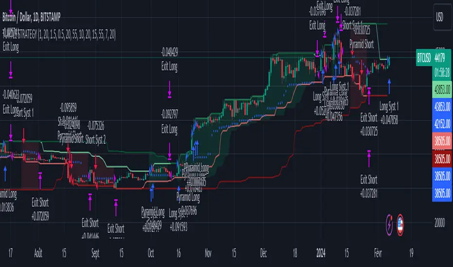
Z-Score Support & Resistance [SS}Hello everyone,
This is the Z-Score Support and Resistance (S/R) indicator.
How it works:
The trouble with most indicators and strategies that rely on distributions is that they are constantly moving targets.
To combat this, what I have done is anchored the assessment of the normal distribution to the period open price and dropped the data from the current day.
This provides us with a static assessment of the current distribution and static target levels.
It then plots out an assessment of what would be neutral (0 Standard Deviations) all the way up to +3 Standard Deviations and all the way down to -3 Standard Deviations.
It can plot out this assessment on any timeframe, from the minutes to the months to the years, simply select which desired timeframe you want in the settings menu (default is 9 which seems to work well for most generic tickers and indicies).
The indicator will also count the number of times a ticker has closed within each designated period. To do this, please make sure that you have the assessment timeframe opened on the chart. So if you want to look at the instances on the daily timeframe, ensure you have the daily timeframe opened. If you want to look on the monthly, ensure you have the monthly opened, etc. (See below):
How to Use:
To use the indicator, its pretty simple.
Simply select the desired timeframe you want to use as S/R and use it!
You can adjust the period lookback from the defaulted 9 period based on:
a) The degree of normality in the dataset (you can use a kurtosis indicator to help you ascertain this); or
b) The back-test results of closes within a desired range.
For the later, you can see an example below:
This is TSLA with a 9 period lookback:
We can see that 50% of closes are happening within 0.5 and -0.5 standard deviations. If we extend this to a 15 period lookback:
Now over 60% of closes are happening in this area.
Why does this matter? Well, because now we know our prime short and long entries (see below):
The green arrows represent prime long setups and the red prime short setups.
This is because we know, 61% of the time the ticker will close between 0.5 and -0.5 standard deviations, so we can trade the ticker back to this area.
Further instructions:
Because it is somewhat of a complex indicator, I have done a tutorial video that I will link below here:
And that is the indicator my friends! Hopefully you enjoy :-).
As always, leave your comments and suggestions / Questions below!
Safe trades!
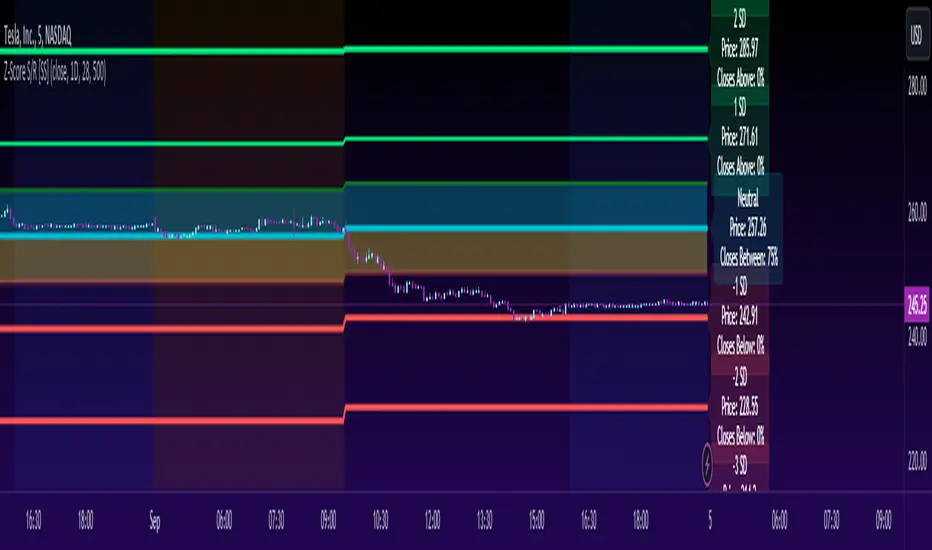
Bullish and Bearish Candlestick Patterns StrategyThe strategy is a combination of candlestick pattern analysis and Fibonacci retracement levels to identify potential buy and sell signals in the market. Here's how the strategy works and how you can trade accordingly:
Candlestick Pattern Analysis:
The strategy looks for specific bullish and bearish candlestick patterns to identify potential trend reversals or continuations. The bullish patterns include:
Bullish Engulfing: This pattern occurs when a bullish candle fully engulfs the previous bearish candle.
Hammer: It is a single candlestick pattern with a small body and a long lower wick, indicating a potential bullish reversal.
Morning Star: This pattern consists of three candles, with the middle one being a small-bodied candle that gaps down and the other two being bullish candles.
The bearish patterns include:
Bearish Engulfing: Similar to the bullish engulfing, but this time, a bearish candle fully engulfs the previous bullish candle.
Shooting Star: A single candlestick pattern with a small body and a long upper wick, suggesting a potential bearish reversal.
Evening Star: This pattern is the opposite of the morning star, with a small-bodied candle that gaps up between two bearish candles.
Fibonacci Retracement Levels:
The strategy uses Fibonacci retracement levels to determine potential support and resistance levels in the market. The main level considered in this strategy is the Fibonacci 0.5 level, which is the midpoint of the previous swing move.
Trading Accordingly:
To trade using this strategy, follow these steps:
a. Observe the Chart: Apply the indicator to your preferred chart, and observe the candlestick patterns and the plotted support, resistance, and Fibonacci 0.5 levels.
b. Buy Signal: A buy signal is generated when any of the bullish candlestick patterns (Bullish Engulfing, Hammer, Morning Star) occur, and the low price of the current candle is above or equal to the Fibonacci 0.5 level. This suggests a potential bullish reversal or continuation of an existing uptrend.
c. Sell Signal: A sell signal is generated when any of the bearish candlestick patterns (Bearish Engulfing, Shooting Star, Evening Star) occur, and the high price of the current candle is below or equal to the Fibonacci 0.5 level. This indicates a potential bearish reversal or continuation of an existing downtrend.
d. Risk Management: Place stop-loss orders to protect your position in case the market moves against your trade. Consider setting the stop-loss below the recent swing low for buy trades and above the recent swing high for sell trades.
e. Take Profit: Set a target for taking profits based on your risk-reward ratio. You can use the recent swing high for buy trades as a potential target and the recent swing low for sell trades.
f. Filter Signals: Keep in mind that not all signals will result in profitable trades. It's essential to filter signals with other technical analysis tools and consider the overall market context.
Remember that no trading strategy guarantees profits, and trading always carries inherent risks. It's crucial to practice proper risk management, use appropriate position sizing, and test the strategy thoroughly in a demo environment before applying it to live trading. Additionally, consider combining this strategy with other indicators or analysis methods to make more informed .
