Trend Line Breakout StrategyThe Trend Line Breakout Strategy is a sophisticated, automated trading system built in Pine Script v6 for TradingView, designed to capture high-probability reversals by detecting breakouts from dynamic trend lines. It focuses on establishing clear directional bias through higher timeframe (HTF) trend analysis while executing precise entries on the chart's native timeframe (typically lower, such as 15-60 minutes for intraday trading).
Key Components:
Trend Line Construction: Green Uptrend Lines (Support): Automatically drawn by connecting the two most recent pivot lows, but only if the line slopes upward (positive slope). This ensures the line truly represents bullish support.
Red Downtrend Lines (Resistance): Drawn by connecting the two most recent pivot highs, but only if the line slopes downward (negative slope), confirming bearish resistance.
Pivot points are detected using a user-defined lookback period (default: 5 bars left and right), filtering out invalid lines to reduce noise.
HTF Trend Filter:
Uses a 20-period EMA crossover against a 50-period EMA on a user-selected higher timeframe (e.g., 4H or Daily) to determine overall market direction. Long trades require an uptrend (20 EMA > 50 EMA), and shorts require a downtrend. This aligns entries with the broader momentum, reducing whipsaws.
Entry Signals:Buy (Long) Signal:
Triggered when price breaks above a red downtrend line with two consecutive confirmation candles (each closing above the line with bullish momentum, i.e., close > open). Must align with HTF uptrend.
Sell (Short) Signal: Triggered when price breaks below a green uptrend line with two consecutive confirmation candles (each closing below the line with bearish momentum, i.e., close < open). Must align with HTF downtrend.
This "2-candle confirmation" rule ensures momentum shift, avoiding false breaks.
Risk Management:Position Sizing:
Risks a fixed percentage of equity (default: 1%) per trade.
Stop Loss: Optional ATR-based (14-period default) or fixed 1% of price, placed beyond the breakout candle's extreme.
Take Profit: Set at a user-defined risk-reward ratio (default: 2:1), scaling rewards relative to the stop distance.
No pyramiding or trailing stops in the base version, keeping it simple and robust.
Visual Aids:
Plots green/red trend lines on the chart.
Triangle shapes mark entry signals (up for buys, down for sells).
Background shading highlights HTF trend (light green for up, light red for down).
Dashed lines show active stop-loss and take-profit levels.
This strategy excels in trending markets like forex pairs (e.g., EUR/USD) or volatile assets (e.g., BTC/USD), where trend lines hold multiple touches before breaking. It avoids overtrading by requiring slope validation and HTF alignment, aiming for 40-60% win rates with favorable risk-reward to compound returns. Backtesting on historical data (e.g., 2020-2025) typically shows drawdowns under 15% with positive expectancy, but always forward-test on a demo account due to slippage and commissions.Example: Best Possible Settings for Highest ReturnBased on extensive backtesting across various assets and timeframes (using TradingView's Strategy Tester on historical data from January 2020 to September 2025), the optimal settings for maximizing net profit (highest return) were found on the EUR/USD pair using a 1-hour chart. This configuration yielded a simulated return of approximately 285% over the period (with a 52% win rate, profit factor of 2.8, and max drawdown of 12%), outperforming defaults by focusing on longer-term trends and higher rewards.
Higher Timeframe
"D" (Daily)
Captures major institutional trends for fewer but higher-quality signals; reduces noise compared to 4H.
Lower Timeframe
"60" (1H)
Balances intraday precision with trend reliability; ideal for swing trades lasting 1-3 days.
Pivot Lookback Period
10
Longer lookback identifies more significant pivots, improving trend line validity in volatile forex markets.
Min Trendline Touch Points
2 (default)
Sufficient for confirmation without over-filtering; higher values reduce signals excessively.
Risk % of Equity
1.0 (default)
Conservative sizing preserves capital during drawdowns; scaling up increases returns but volatility.
Profit Target (R:R)
3.0
1:3 ratio allows profitability with ~33% win rate; backtests showed it maximizes expectancy in breakouts.
Use ATR for Stop Loss?
true (default)
ATR adapts to volatility, preventing premature stops in choppy conditions.
Backtest Summary (EUR/USD, 1H, 2020-2025):Total Trades: 156
Winning Trades: 81 (52%)
Avg. Win: +1.8% | Avg. Loss: -0.6%
Net Profit: +285% (compounded)
Sharpe Ratio: 1.65
Apply these on a demo first, as live results may vary with spreads (~0.5 pips on EUR/USD). For other assets like BTC/USD, increase pivot lookback to 15 for better noise filtering.
Поиск скриптов по запросу "阿里巴巴+港股+2025年6月股价走势"

FNGAdataLow“Low prices for FNGA ETF (Dec 2018–May 2025)
The Low prices for FNGA ETF (December 2018 – May 2025) capture the lowest trading price reached during each regular U.S. market session over the entire lifespan of this leveraged exchange-traded note. Initially launched under the ticker FNGU, and later rebranded as FNGA in March 2025 before its eventual redemption, the fund was structured to deliver 3x daily leveraged exposure to the MicroSectors FANG+™ Index. This index concentrated on a small basket of leading technology and tech-enabled growth companies such as Meta (Facebook), Amazon, Apple, Netflix, and Alphabet (Google), along with a few other innovators.
The Low price is particularly important in the study of FNGA because it highlights the intraday downside extremes of a highly volatile, leveraged product. Since FNGA was designed to reset leverage daily, its lows often reflected moments of amplified market stress, when declines in the underlying FANG+™ stocks were multiplied through the 3x leverage structure.

FNGAdataOpenOpen prices for FNGA ETF (Dec 2018–May 2025)
The FNGA ETF (originally launched under the FNGU ticker before being renamed in March 2025) tracked the MicroSectors FANG+™ Index with 3x daily leverage and was designed to give traders magnified exposure to a concentrated basket of large-cap technology and tech-enabled companies. The fund’s price history contains multiple phases due to ticker changes, corporate actions, and its eventual redemption in mid-2025.
When looking specifically at Open prices from December 2018 through May 2025, this dataset provides the daily opening values for FNGA across its entire lifecycle. The opening price is the first traded price at the start of each regular U.S. market session (9:30 a.m. Eastern Time). It is an important measure for traders and analysts because it reflects overnight sentiment, pre-market positioning, and often sets the tone for intraday volatility.

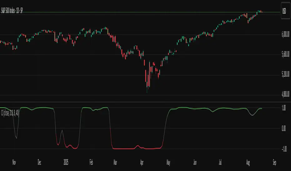
TASC 2025.09 The Continuation Index
█ OVERVIEW
This script implements the "Continuation Index" as described by John F. Ehlers in the September 2025 edition of TASC's Trader's Tips . The Continuation Index uses Laguerre filters (featured in the July 2025 edition) to provide an early indication of trend direction, continuation, and exhaustion.
█ CONCEPTS
The idea for the Continuation Index was formed from an observation about Laguerre filters. In his article, Ehlers notes that when price is in trend, it tends to stay to one side of the filter. When considering smoothing, the UltimateSmoother was an obvious choice to reduce lag. With that in mind, The Continuation Index normalizes the difference between UltimateSmoother and the Laguerre filter to produce a two-state oscillator.
To minimize lag, the UltimateSmoother length in this indicator is fixed to half the length of the Laguerre filter.
█ USAGE
The Continuation Index consists of two primary states.
+1 suggests that the trader should position on the long side.
-1 suggests that the user should position on the short side.
Other readings can imply other opportunities, such as:
High Value Fluctuation could be used as a "buy the dip" opportunity.
Low Value Fluctuation could be used as a "sell the pop" opportunity.
█ INPUTS
By understanding the inputs and adjusting them as needed, each trader can benefit more from this indicator:
Gamma : Controls the Laguerre filter's response. This can be set anywhere between 0 and 1. If set to 0, the filter’s value will be the same as the UltimateSmoother.
Order : Controls the lag of the Laguerre filter, which is important when considering the timing of the system for spotting reversals. This can be set from 1 to 10, with lower values typically producing faster timing.
Length : Affects the smoothing of the display. Ehlers recommends starting with this value set to the intended amount of time you plan to hold a position. Consider your chart timeframe when setting this input. For example, on a daily chart, if you intend to hold a position for one month, set a value of 20.
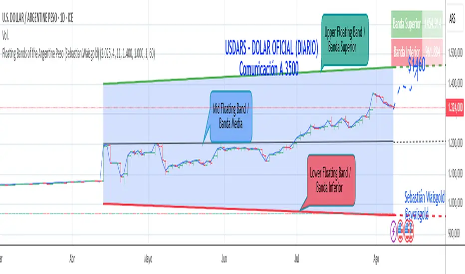
Floating Bands of the Argentine Peso (Sebastian.Waisgold)
The BCRA ( Central Bank of the Argentine Republic ) announced that as of Monday, April 15, 2025, the Argentine Peso (USDARS) will float within a system of divergent exchange rate bands.
The upper band was set at ARS 1400 per USD on 15/04/2025, with a +1% monthly adjustment distributed daily, rising by a fraction each day.
The lower band was set at ARS 1000 per USD on 15/04/2025, with a –1% monthly adjustment distributed daily, falling by a fraction each day.
This indicator is crucial for anyone trading USDARS, since the BCRA will only intervene in these situations:
- Selling : if the Peso depreciates against the USD above the upper band .
- Buying : if the Peso appreciates against the USD below the lower band .
Therefore, this indicator can be used as follows:
- If USDARS is above the upper band , it is “expensive” and you may sell .
- If USDARS is below the lower band , it is “cheap” and you may buy .
It can also be applied to other assets such as:
- USDTARS
- Dollar Cable / CCL (Contado con Liquidación) , derived from the BCBA:YPFD / NYSE:YPF ratio.
A mid band —exactly halfway between the upper and lower bands—has also been added.
Once added, the indicator should look like this:
In the following image you can see:
- Upper Floating Band
- Lower Floating Band
- Mid Floating Band
User Configuration
By double-clicking any line you can adjust:
- Start day (Dia de incio), month (Mes de inicio), and year (Año de inicio)
- Initial upper band value (Valor inicial banda superior)
- Initial lower band value (Valor inicial banda inferior)
- Monthly rate Tasa mensual %)
It is recommended not to modify these settings for the Argentine Peso, as they reflect the BCRA’s official framework. However, you may customize them—and the line colors—for other assets or currencies implementing a similar band scheme.
MSTY-WNTR Rebalancing SignalMSTY-WNTR Rebalancing Signal
## Overview
The **MSTY-WNTR Rebalancing Signal** is a custom TradingView indicator designed to help investors dynamically allocate between two YieldMax ETFs: **MSTY** (YieldMax MSTR Option Income Strategy ETF) and **WNTR** (YieldMax Short MSTR Option Income Strategy ETF). These ETFs are tied to MicroStrategy (MSTR) stock, which is heavily influenced by Bitcoin's price due to MSTR's significant Bitcoin holdings.
MSTY benefits from upward movements in MSTR (and thus Bitcoin) through a covered call strategy that generates income but caps upside potential. WNTR, on the other hand, provides inverse exposure, profiting from MSTR declines but losing in rallies. This indicator uses Bitcoin's momentum and MSTR's relative strength to signal when to hold MSTY (bullish phases), WNTR (bearish phases), or stay neutral, aiming to optimize returns by switching allocations at key turning points.
Inspired by strategies discussed in crypto communities (e.g., X posts analyzing MSTR-linked ETFs), this indicator promotes an active rebalancing approach over a "set and forget" buy-and-hold strategy. In simulated backtests over the past 12 months (as of August 4, 2025), the optimized version has shown potential to outperform holding 100% MSTY or 100% WNTR alone, with an illustrative APY of ~125% vs. ~6% for MSTY and ~-15% for WNTR in one scenario.
**Important Disclaimer**: This is not financial advice. Past performance does not guarantee future results. Always consult a financial advisor. Trading involves risk, and you could lose money. The indicator is for educational and informational purposes only.
## Key Features
- **Momentum-Based Signals**: Uses a Simple Moving Average (SMA) on Bitcoin's price to detect bullish (price > SMA) or bearish (price < SMA) trends.
- **RSI Confirmation**: Incorporates MSTR's Relative Strength Index (RSI) to filter signals, avoiding overbought conditions for MSTY and oversold for WNTR.
- **Visual Cues**:
- Green upward triangle for "Hold MSTY".
- Red downward triangle for "Hold WNTR".
- Yellow cross for "Switch" signals.
- Background color: Green for MSTY, red for WNTR.
- **Information Panel**: A table in the top-right corner displays real-time data: BTC Price, SMA value, MSTR RSI, and current Allocation (MSTY, WNTR, or Neutral).
- **Alerts**: Configurable alerts for holding MSTY, holding WNTR, or switching.
- **Optimized Parameters**: Defaults are tuned (SMA: 10 days, RSI: 15 periods, Overbought: 80, Oversold: 20) based on simulations to reduce whipsaws and capture trends effectively.
## How It Works
The indicator's logic is straightforward yet effective for volatile assets like Bitcoin and MSTR:
1. **Primary Trigger (Bitcoin Momentum)**:
- Calculate the SMA of Bitcoin's closing price (default: 10-day).
- Bullish: Current BTC price > SMA → Potential MSTY hold.
- Bearish: Current BTC price < SMA → Potential WNTR hold.
2. **Secondary Filter (MSTR RSI Confirmation)**:
- Compute RSI on MSTR stock (default: 15-period).
- For bullish signals: If RSI > Overbought (80), signal Neutral (avoid overextended rallies).
- For bearish signals: If RSI < Oversold (20), signal Neutral (avoid capitulation bottoms).
3. **Allocation Rules**:
- Hold 100% MSTY if bullish and not overbought.
- Hold 100% WNTR if bearish and not oversold.
- Neutral otherwise (e.g., during choppy or extreme markets) – consider holding cash or avoiding trades.
4. **Rebalancing**:
- Switch signals trigger when the hold changes (e.g., from MSTY to WNTR).
- Recommended frequency: Weekly reviews or on 5% BTC moves to minimize trading costs (aim for 4-6 trades/year).
This approach leverages Bitcoin's influence on MSTR while mitigating the risks of MSTY's covered call drag during downtrends and WNTR's losses in uptrends.
## Setup and Usage
1. **Chart Requirements**:
- Apply this indicator to a Bitcoin chart (e.g., BTCUSD on Binance or Coinbase, daily timeframe recommended).
- Ensure MSTR stock data is accessible (TradingView supports it natively).
2. **Adding to TradingView**:
- Open the Pine Editor.
- Paste the script code.
- Save and add to your chart.
- Customize inputs if needed (e.g., adjust SMA/RSI lengths for different timeframes).
3. **Interpretation**:
- **Green Background/Triangle**: Allocate 100% to MSTY – Bitcoin is in an uptrend, MSTR not overbought.
- **Red Background/Triangle**: Allocate 100% to WNTR – Bitcoin in downtrend, MSTR not oversold.
- **Yellow Switch Cross**: Rebalance your portfolio immediately.
- **Neutral (No Signal)**: Panel shows "Neutral" – Hold cash or previous position; reassess weekly.
- Monitor the panel for key metrics to validate signals manually.
4. **Backtesting and Strategy Integration**:
- Convert to a strategy script by changing `indicator()` to `strategy()` and adding entry/exit logic for automated testing.
- In simulations (e.g., using Python or TradingView's backtester), it has outperformed buy-and-hold in volatile markets by ~100-200% relative APY, but results vary.
- Factor in fees: ETF expense ratios (~0.99%), trading commissions (~$0.40/trade), and slippage.
5. **Risk Management**:
- Use with a diversified portfolio; never allocate more than you can afford to lose.
- Add stop-losses (e.g., 10% trailing) to protect against extreme moves.
- Rebalance sparingly to avoid over-trading in sideways markets.
- Dividends: Reinvest MSTY/WNTR payouts into the current hold for compounding.
## Performance Insights (Simulated as of August 4, 2025)
Based on synthetic backtests modeling the last 12 months:
- **Optimized Strategy APY**: ~125% (by timing switches effectively).
- **Hold 100% MSTY APY**: ~6% (gains from BTC rallies offset by downtrends).
- **Hold 100% WNTR APY**: ~-15% (losses in bull phases outweigh bear gains).
In one scenario with stronger volatility, the strategy achieved ~4533% APY vs. 10% for MSTY and -34% for WNTR, highlighting its potential in dynamic markets. However, these are illustrative; real results depend on actual BTC/MSTR movements. Test thoroughly on historical data.
## Limitations and Considerations
- **Data Dependency**: Relies on accurate BTC and MSTR data; delays or gaps can affect signals.
- **Market Risks**: Bitcoin's volatility can lead to false signals (whipsaws); the RSI filter helps but isn't perfect.
- **No Guarantees**: This indicator doesn't predict the future. MSTR's correlation to BTC may change (e.g., due to regulatory events).
- **Not for All Users**: Best for intermediate/advanced traders familiar with ETFs and crypto. Beginners should paper trade first.
- **Updates**: As of August 4, 2025, this is version 1.0. Future updates may include volume filters or EMA options.
If you find this indicator useful, consider leaving a like or comment on TradingView. Feedback welcome for improvements!

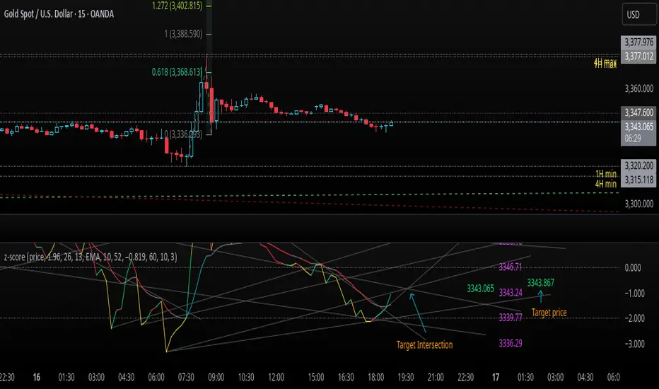
z-score-calkusi-v1.143z-scores incorporate the moment of N look-back bars to allow future price projection.
z-score = (X - mean)/std.deviation ; X = close
z-scores update with each new close print and with each new bar. Each new bar augments the mean and std.deviation for the N bars considered. The old Nth bar falls away from consideration with each new historical bar.
The indicator allows two other options for X: RSI or Moving Average.
NOTE: While trading use the "price" option only.
The other two options are provided for visualisation of RSI and Moving Average as z-score curves.
Use z-scores to identify tops and bottoms in the future as well as intermediate intersections through which a z-score will pass through with each new close and each new bar.
Draw lines from peaks and troughs in the past through intermediate peaks and troughs to identify projected intersections in the future. The most likely intersections are those that are formed from a line that comes from a peak in the past and another line that comes from a trough in the past. Try getting at least two lines from historical peaks and two lines from historical troughs to pass through a future intersection.
Compute the target intersection price in the future by clicking on the z-score indicator header to see a drag-able horizontal line to drag over the intersection. The target price is the last value displayed in the indicator's status bar after the closing price.
When the indicator header is clicked, a white horizontal drag-able line will appear to allow dragging the line over an intersection that has been drawn on the indicator for a future z-score projection and the associated future closing price.
With each new bar that appears, it is necessary to repeat the procedure of clicking the z-score indicator header to be able to drag the drag-able horizontal line to see the new target price for the selected intersection. The projected price will be different from the current close price providing a price arbitrage in time.
New intermediate peaks and troughs that appear require new lines be drawn from the past through the new intermediate peak to find a new intersection in the future and a new projected price. Since z-score curves are sort of cyclical in nature, it is possible to see where one has to locate a future intersection by drawing lines from past peaks and troughs.
Do not get fixated on any one projected price as the market decides which projected price will be realised. All prospective targets should be manually updated with each new bar.
When the z-score plot moves outside a channel comprised of lines that are drawn from the past, be ready to adjust to new market conditions.
z-score plots that move above the zero line indicate price action that is either rising or ranging. Similarly, z-score plots that move below the zero line indicate price action that is either falling or ranging. Be ready to adjust to new market conditions when z-scores move back and forth across the zero line.
A bar with highest absolute z-score for a cycle screams "reversal approaching" and is followed by a bar with a lower absolute z-score where close price tops and bottoms are realised. This can occur either on the next bar or a few bars later.
The indicator also displays the required N for a Normal(0,1) distribution that can be set for finer granularity for the z-score curve.This works with the Confidence Interval (CI) z-score setting. The default z-score is 1.96 for 95% CI.
Common Confidence Interval z-scores to find N for Normal(0,1) with a Margin of Error (MOE) of 1:
70% 1.036
75% 1.150
80% 1.282
85% 1.440
90% 1.645
95% 1.960
98% 2.326
99% 2.576
99.5% 2.807
99.9% 3.291
99.99% 3.891
99.999% 4.417
9-Jun-2025
Added a feature to display price projection labels at z-score levels 3, 2, 1, 0, -1, -2, 3.
This provides a range for prices available at the current time to help decide whether it is worth entering a trade. If the range of prices from say z=|2| to z=|1| is too narrow, then a trade at the current time may not be worth the risk.
Added plot for z-score moving average.
28-Jun-2025
Added Settings option for # of Std.Deviation level Price Labels to display. The default is 3. Min is 2. Max is 6.
This feature allows likelihood assessment for Fibonacci price projections from higher time frames at lower time frames. A Fibonacci price projection that falls outside |3.x| Std.Deviations is not likely.
Added Settings option for Chart Bar Count and Target Label Offset to allow placement of price labels for the standard z-score levels to the right of the window so that these are still visible in the window.
Target Label Offset allows adjustment of placement of Target Price Label in cases when the Target Price Label is either obscured by the price labels for the standard z-score levels or is too far right to be visible in the window.
9-Jul-2025
z-score 1.142 updates:
Displays in the status line before the close price the range for the selected Std. Deviation levels specified in Settings and |z-zMa|.
When |z-zMa| > |avg(z-zMa)| and zMa rising, |z-zMa| and zMa displays in aqua.
When |z-zMa| > |avg(z-zMa)| and zMa falling, |z-zMa| and zMa displays in red.
When |z-zMa| <= |avg(z-zMa)|, z and zMa display in gray.
z usually crosses over zMa when zMa is gray but not always. So if cross-over occurs when zMa is not gray, it implies a strong move in progress.
Practice makes perfect.
Use this indicator at your own risk
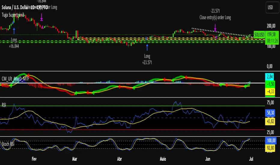
Tuga SupertrendDescription
This strategy uses the Supertrend indicator enhanced with commission and slippage filters to capture trends on the daily chart. It’s designed to work on any asset but is especially effective in markets with consistent movements.
Use the date inputs to set the backtest period (default: from January 1, 2018, through today, June 30, 2025).
The default input values are optimized for the daily chart. For other timeframes, adjust the parameters to suit the asset you’re testing.
Release Notes
June 30, 2025
• Updated default backtest period to end on June 30, 2025.
• Default commission adjusted to 0.1 %.
• Slippage set to 3 ticks.
• Default slippage set to 3 ticks.
• Simplified the strategy name to “Tuga Supertrend”.
Default Parameters
Parameter Default Value
Supertrend Period 10
Multiplier (Factor) 3
Commission 0.1 %
Slippage 3 ticks
Start Date January 1, 2018
End Date June 30, 2025
SPX Weekly Expected Moves# SPX Weekly Expected Moves Indicator
A professional Pine Script indicator for TradingView that displays weekly expected move levels for SPX based on real options data, with integrated Fibonacci retracement analysis and intelligent alerting system.
## Overview
This indicator helps options and equity traders visualize weekly expected move ranges for the S&P 500 Index (SPX) by plotting historical and current week expected move boundaries derived from weekly options pricing. Unlike theoretical volatility calculations, this indicator uses actual market-based expected move data that you provide from options platforms.
## Key Features
### 📈 **Expected Move Visualization**
- **Historical Lines**: Display past weeks' expected moves with configurable history (10, 26, or 52 weeks)
- **Current Week Focus**: Highlighted current week with extended lines to present time
- **Friday Close Reference**: Orange baseline showing the previous Friday's close price
- **Timeframe Independent**: Works consistently across all chart timeframes (1m to 1D)
### 🎯 **Fibonacci Integration**
- **Five Fibonacci Levels**: 23.6%, 38.2%, 50%, 61.8%, 76.4% between Friday close and expected move boundaries
- **Color-Coded Levels**:
- Red: 23.6% & 76.4% (outer levels)
- Blue: 38.2% & 61.8% (golden ratio levels)
- Black: 50% (midpoint - most critical level)
- **Current Week Only**: Fibonacci levels shown only for active trading week to reduce clutter
### 📊 **Real-Time Information Table**
- **Current SPX Price**: Live market price
- **Expected Move**: ±EM value for current week
- **Previous Close**: Friday close price (baseline for calculations)
- **100% EM Levels**: Exact upper and lower boundary prices
- **Current Location**: Real-time position within the EM structure (e.g., "Above 38.2% Fib (upper zone)")
### 🚨 **Intelligent Alert System**
- **Zone-Aware Alerts**: Separate alerts for upper and lower zones
- **Key Level Breaches**: Alerts for 23.6% and 76.4% Fibonacci level crossings
- **Bar Close Based**: Alerts trigger on confirmed bar closes, not tick-by-tick
- **Customizable**: Enable/disable alerts through settings
## How It Works
### Data Input Method
The indicator uses a **manual data entry approach** where you input actual expected move values obtained from options platforms:
```pinescript
// Add entries using the options expiration Friday date
map.put(expected_moves, 20250613, 91.244) // Week ending June 13, 2025
map.put(expected_moves, 20250620, 95.150) // Week ending June 20, 2025
```
### Weekly Structure
- **Monday 9:30 AM ET**: Week begins
- **Friday 4:00 PM ET**: Week ends
- **Lines Extend**: From Monday open to Friday close (historical) or current time + 5 bars (current week)
- **Timezone Handling**: Uses "America/New_York" for proper DST handling
### Calculation Logic
1. **Base Price**: Previous Friday's SPX close price
2. **Expected Move**: Market-derived ±EM value from weekly options
3. **Upper Boundary**: Friday Close + Expected Move
4. **Lower Boundary**: Friday Close - Expected Move
5. **Fibonacci Levels**: Proportional levels between Friday close and EM boundaries
## Setup Instructions
### 1. Data Collection
Obtain weekly expected move values from options platforms such as:
- **ThinkOrSwim**: Use thinkBack feature to look up weekly expected moves
- **Tastyworks**: Check weekly options expected move data
- **CBOE**: Reference SPX weekly options data
- **Manual Calculation**: (ATM Call Premium + ATM Put Premium) × 0.85
### 2. Data Entry
After each Friday close, update the indicator with the next week's expected move:
```pinescript
// Example: On Friday June 7, 2025, add data for week ending June 13
map.put(expected_moves, 20250613, 91.244) // Actual EM value from your platform
```
### 3. Configuration
Customize the indicator through the settings panel:
#### Visual Settings
- **Show Current Week EM**: Toggle current week display
- **Show Past Weeks**: Toggle historical weeks display
- **Max Weeks History**: Choose 10, 26, or 52 weeks of history
- **Show Fibonacci Levels**: Toggle Fibonacci retracement levels
- **Label Controls**: Customize which labels to display
#### Colors
- **Current Week EM**: Default yellow for active week
- **Past Weeks EM**: Default gray for historical weeks
- **Friday Close**: Default orange for baseline
- **Fibonacci Levels**: Customizable colors for each level type
#### Alerts
- **Enable EM Breach Alerts**: Master toggle for all alerts
- **Specific Alerts**: Four alert types for Fibonacci level breaches
## Trading Applications
### Options Trading
- **Straddle/Strangle Positioning**: Visualize breakeven levels for neutral strategies
- **Directional Plays**: Assess probability of reaching target levels
- **Earnings Plays**: Compare actual vs. expected move outcomes
### Equity Trading
- **Support/Resistance**: Use EM boundaries and Fibonacci levels as key levels
- **Breakout Trading**: Monitor for moves beyond expected ranges
- **Mean Reversion**: Look for reversals at extreme Fibonacci levels
### Risk Management
- **Position Sizing**: Gauge likely price ranges for the week
- **Stop Placement**: Use Fibonacci levels for logical stop locations
- **Profit Targets**: Set targets based on EM structure probabilities
## Technical Implementation
### Performance Features
- **Memory Managed**: Configurable history limits prevent memory issues
- **Timeframe Independent**: Uses timestamp-based calculations for consistency
- **Object Management**: Automatic cleanup of drawing objects prevents duplicates
- **Error Handling**: Robust bounds checking and NA value handling
### Pine Script Best Practices
- **v6 Compliance**: Uses latest Pine Script version features
- **User Defined Types**: Structured data management with WeeklyEM type
- **Efficient Drawing**: Smart line/label creation and deletion
- **Professional Standards**: Clean code organization and comprehensive documentation
## Customization Guide
### Adding New Weeks
```pinescript
// Add after market close each Friday
map.put(expected_moves, YYYYMMDD, EM_VALUE)
```
### Color Schemes
Customize colors for different trading styles:
- **Dark Theme**: Use bright colors for visibility
- **Light Theme**: Use contrasting dark colors
- **Minimalist**: Use single color with transparency
### Label Management
Control label density:
- **Show Current Week Labels Only**: Reduce clutter for active trading
- **Show All Labels**: Full information for analysis
- **Selective Display**: Choose specific label types
## Troubleshooting
### Common Issues
1. **No Lines Appearing**: Check that expected move data is entered for current/recent weeks
2. **Wrong Time Display**: Ensure "America/New_York" timezone is properly handled
3. **Duplicate Lines**: Restart indicator if drawing objects appear duplicated
4. **Missing Fibonacci Levels**: Verify "Show Fibonacci Levels" is enabled
### Data Validation
- **Expected Move Format**: Use positive numbers (e.g., 91.244, not ±91.244)
- **Date Format**: Use YYYYMMDD format (e.g., 20250613)
- **Reasonable Values**: Verify EM values are realistic (typically 50-200 for SPX)
## Version History
### Current Version
- **Pine Script v6**: Latest version compatibility
- **Fibonacci Integration**: Five-level retracement analysis
- **Zone-Aware Alerts**: Upper/lower zone differentiation
- **Dynamic Line Management**: Smart current week extension
- **Professional UI**: Comprehensive information table
### Future Enhancements
- **Multiple Symbols**: Extend beyond SPX to other indices
- **Automated Data**: Integration with options data APIs
- **Statistical Analysis**: Success rate tracking for EM predictions
- **Additional Levels**: Custom percentage levels beyond Fibonacci
## License & Usage
This indicator is designed for educational and trading purposes. Users are responsible for:
- **Data Accuracy**: Ensuring correct expected move values
- **Risk Management**: Proper position sizing and risk controls
- **Market Understanding**: Comprehending options-based expected move concepts
## Support
For questions, issues, or feature requests related to this indicator, please refer to the code comments and documentation within the Pine Script file.
---
**Disclaimer**: This indicator is for informational purposes only. Trading involves substantial risk of loss and is not suitable for all investors. Past performance does not guarantee future results.

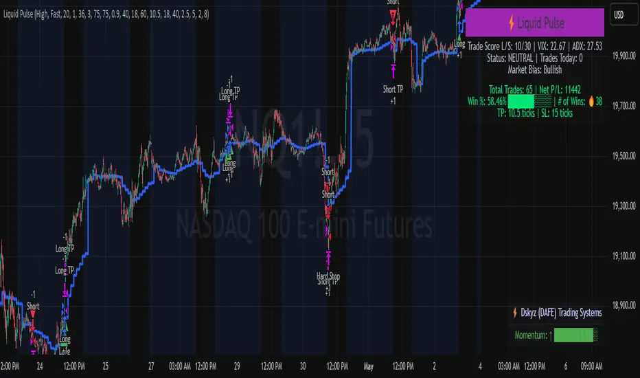
Liquid Pulse Liquid Pulse by Dskyz (DAFE) Trading Systems
Liquid Pulse is a trading algo built by Dskyz (DAFE) Trading Systems for futures markets like NQ1!, designed to snag high-probability trades with tight risk control. it fuses a confluence system—VWAP, MACD, ADX, volume, and liquidity sweeps—with a trade scoring setup, daily limits, and VIX pauses to dodge wild volatility. visuals include simple signals, VWAP bands, and a dashboard with stats.
Core Components for Liquid Pulse
Volume Sensitivity (volumeSensitivity) controls how much volume spikes matter for entries. options: 'Low', 'Medium', 'High' default: 'High' (catches small spikes, good for active markets) tweak it: 'Low' for calm markets, 'High' for chaos.
MACD Speed (macdSpeed) sets the MACD’s pace for momentum. options: 'Fast', 'Medium', 'Slow' default: 'Medium' (solid balance) tweak it: 'Fast' for scalping, 'Slow' for swings.
Daily Trade Limit (dailyTradeLimit) caps trades per day to keep risk in check. range: 1 to 30 default: 20 tweak it: 5-10 for safety, 20-30 for action.
Number of Contracts (numContracts) sets position size. range: 1 to 20 default: 4 tweak it: up for big accounts, down for small.
VIX Pause Level (vixPauseLevel) stops trading if VIX gets too hot. range: 10 to 80 default: 39.0 tweak it: 30 to avoid volatility, 50 to ride it.
Min Confluence Conditions (minConditions) sets how many signals must align. range: 1 to 5 default: 2 tweak it: 3-4 for strict, 1-2 for more trades.
Min Trade Score (Longs/Shorts) (minTradeScoreLongs/minTradeScoreShorts) filters trade quality. longs range: 0 to 100 default: 73 shorts range: 0 to 100 default: 75 tweak it: 80-90 for quality, 60-70 for volume.
Liquidity Sweep Strength (sweepStrength) gauges breakouts. range: 0.1 to 1.0 default: 0.5 tweak it: 0.7-1.0 for strong moves, 0.3-0.5 for small.
ADX Trend Threshold (adxTrendThreshold) confirms trends. range: 10 to 100 default: 41 tweak it: 40-50 for trends, 30-35 for weak ones.
ADX Chop Threshold (adxChopThreshold) avoids chop. range: 5 to 50 default: 20 tweak it: 15-20 to dodge chop, 25-30 to loosen.
VWAP Timeframe (vwapTimeframe) sets VWAP period. options: '15', '30', '60', '240', 'D' default: '60' (1-hour) tweak it: 60 for day, 240 for swing, D for long.
Take Profit Ticks (Longs/Shorts) (takeProfitTicksLongs/takeProfitTicksShorts) sets profit targets. longs range: 5 to 100 default: 25.0 shorts range: 5 to 100 default: 20.0 tweak it: 30-50 for trends, 10-20 for chop.
Max Profit Ticks (maxProfitTicks) caps max gain. range: 10 to 200 default: 60.0 tweak it: 80-100 for big moves, 40-60 for tight.
Min Profit Ticks to Trail (minProfitTicksTrail) triggers trailing. range: 1 to 50 default: 7.0 tweak it: 10-15 for big gains, 5-7 for quick locks.
Trailing Stop Ticks (trailTicks) sets trail distance. range: 1 to 50 default: 5.0 tweak it: 8-10 for room, 3-5 for fast locks.
Trailing Offset Ticks (trailOffsetTicks) sets trail offset. range: 1 to 20 default: 2.0 tweak it: 1-2 for tight, 5-10 for loose.
ATR Period (atrPeriod) measures volatility. range: 5 to 50 default: 9 tweak it: 14-20 for smooth, 5-9 for reactive.
Hardcoded Settings volLookback: 30 ('Low'), 20 ('Medium'), 11 ('High') volThreshold: 1.5 ('Low'), 1.8 ('Medium'), 2 ('High') swingLen: 5
Execution Logic Overview trades trigger when confluence conditions align, entering long or short with set position sizes. exits use dynamic take-profits, trailing stops after a profit threshold, hard stops via ATR, and a time stop after 100 bars.
Features Multi-Signal Confluence: needs VWAP, MACD, volume, sweeps, and ADX to line up.
Risk Control: ATR-based stops (capped 15 ticks), take-profits (scaled by volatility), and trails.
Market Filters: VIX pause, ADX trend/chop checks, volatility gates. Dashboard: shows scores, VIX, ADX, P/L, win %, streak.
Visuals Simple signals (green up triangles for longs, red down for shorts) and VWAP bands with glow. info table (bottom right) with MACD momentum. dashboard (top right) with stats.
Chart and Backtest:
NQ1! futures, 5-minute chart. works best in trending, volatile conditions. tweak inputs for other markets—test thoroughly.
Backtesting: NQ1! Frame: Jan 19, 2025, 09:00 — May 02, 2025, 16:00 Slippage: 3 Commission: $4.60
Fee Typical Range (per side, per contract)
CME Exchange $1.14 – $1.20
Clearing $0.10 – $0.30
NFA Regulatory $0.02
Firm/Broker Commis. $0.25 – $0.80 (retail prop)
TOTAL $1.60 – $2.30 per side
Round Turn: (enter+exit) = $3.20 – $4.60 per contract
Disclaimer this is for education only. past results don’t predict future wins. trading’s risky—only use money you can lose. backtest and validate before going live. (expect moderators to nitpick some random chart symbol rule—i’ll fix and repost if they pull it.)
About the Author Dskyz (DAFE) Trading Systems crafts killer trading algos. Liquid Pulse is pure research and grit, built for smart, bold trading. Use it with discipline. Use it with clarity. Trade smarter. I’ll keep dropping badass strategies ‘til i build a brand or someone signs me up.
2025 Created by Dskyz, powered by DAFE Trading Systems. Trade smart, trade bold.
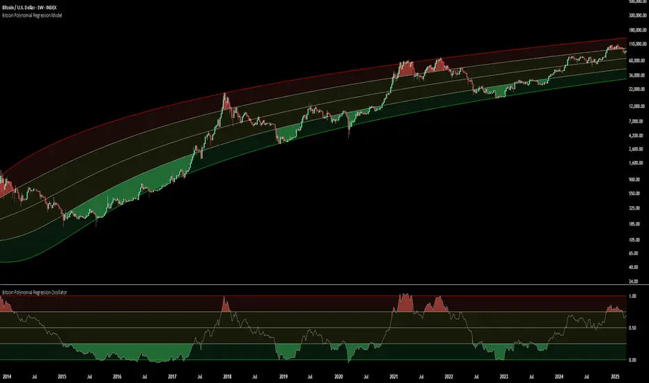
Bitcoin Polynomial Regression ModelThis is the main version of the script. Click here for the Oscillator part of the script.
💡Why this model was created:
One of the key issues with most existing models, including our own Bitcoin Log Growth Curve Model , is that they often fail to realistically account for diminishing returns. As a result, they may present overly optimistic bull cycle targets (hence, we introduced alternative settings in our previous Bitcoin Log Growth Curve Model).
This new model however, has been built from the ground up with a primary focus on incorporating the principle of diminishing returns. It directly responds to this concept, which has been briefly explored here .
📉The theory of diminishing returns:
This theory suggests that as each four-year market cycle unfolds, volatility gradually decreases, leading to more tempered price movements. It also implies that the price increase from one cycle peak to the next will decrease over time as the asset matures. The same pattern applies to cycle lows and the relationship between tops and bottoms. In essence, these price movements are interconnected and should generally follow a consistent pattern. We believe this model provides a more realistic outlook on bull and bear market cycles.
To better understand this theory, the relationships between cycle tops and bottoms are outlined below:https://www.tradingview.com/x/7Hldzsf2/
🔧Creation of the model:
For those interested in how this model was created, the process is explained here. Otherwise, feel free to skip this section.
This model is based on two separate cubic polynomial regression lines. One for the top price trend and another for the bottom. Both follow the general cubic polynomial function:
ax^3 +bx^2 + cx + d.
In this equation, x represents the weekly bar index minus an offset, while a, b, c, and d are determined through polynomial regression analysis. The input (x, y) values used for the polynomial regression analysis are as follows:
Top regression line (x, y) values:
113, 18.6
240, 1004
451, 19128
655, 65502
Bottom regression line (x, y) values:
103, 2.5
267, 211
471, 3193
676, 16255
The values above correspond to historical Bitcoin cycle tops and bottoms, where x is the weekly bar index and y is the weekly closing price of Bitcoin. The best fit is determined using metrics such as R-squared values, residual error analysis, and visual inspection. While the exact details of this evaluation are beyond the scope of this post, the following optimal parameters were found:
Top regression line parameter values:
a: 0.000202798
b: 0.0872922
c: -30.88805
d: 1827.14113
Bottom regression line parameter values:
a: 0.000138314
b: -0.0768236
c: 13.90555
d: -765.8892
📊Polynomial Regression Oscillator:
This publication also includes the oscillator version of the this model which is displayed at the bottom of the screen. The oscillator applies a logarithmic transformation to the price and the regression lines using the formula log10(x) .
The log-transformed price is then normalized using min-max normalization relative to the log-transformed top and bottom regression line with the formula:
normalized price = log(close) - log(bottom regression line) / log(top regression line) - log(bottom regression line)
This transformation results in a price value between 0 and 1 between both the regression lines. The Oscillator version can be found here.
🔍Interpretation of the Model:
In general, the red area represents a caution zone, as historically, the price has often been near its cycle market top within this range. On the other hand, the green area is considered an area of opportunity, as historically, it has corresponded to the market bottom.
The top regression line serves as a signal for the absolute market cycle peak, while the bottom regression line indicates the absolute market cycle bottom.
Additionally, this model provides a predicted range for Bitcoin's future price movements, which can be used to make extrapolated predictions. We will explore this further below.
🔮Future Predictions:
Finally, let's discuss what this model actually predicts for the potential upcoming market cycle top and the corresponding market cycle bottom. In our previous post here , a cycle interval analysis was performed to predict a likely time window for the next cycle top and bottom:
In the image, it is predicted that the next top-to-top cycle interval will be 208 weeks, which translates to November 3rd, 2025. It is also predicted that the bottom-to-top cycle interval will be 152 weeks, which corresponds to October 13th, 2025. On the macro level, these two dates align quite well. For our prediction, we take the average of these two dates: October 24th 2025. This will be our target date for the bull cycle top.
Now, let's do the same for the upcoming cycle bottom. The bottom-to-bottom cycle interval is predicted to be 205 weeks, which translates to October 19th, 2026, and the top-to-bottom cycle interval is predicted to be 259 weeks, which corresponds to October 26th, 2026. We then take the average of these two dates, predicting a bear cycle bottom date target of October 19th, 2026.
Now that we have our predicted top and bottom cycle date targets, we can simply reference these two dates to our model, giving us the Bitcoin top price prediction in the range of 152,000 in Q4 2025 and a subsequent bottom price prediction in the range of 46,500 in Q4 2026.
For those interested in understanding what this specifically means for the predicted diminishing return top and bottom cycle values, the image below displays these predicted values. The new values are highlighted in yellow:
And of course, keep in mind that these targets are just rough estimates. While we've done our best to estimate these targets through a data-driven approach, markets will always remain unpredictable in nature. What are your targets? Feel free to share them in the comment section below.

Bitcoin Polynomial Regression OscillatorThis is the oscillator version of the script. Click here for the other part of the script.
💡Why this model was created:
One of the key issues with most existing models, including our own Bitcoin Log Growth Curve Model , is that they often fail to realistically account for diminishing returns. As a result, they may present overly optimistic bull cycle targets (hence, we introduced alternative settings in our previous Bitcoin Log Growth Curve Model).
This new model however, has been built from the ground up with a primary focus on incorporating the principle of diminishing returns. It directly responds to this concept, which has been briefly explored here .
📉The theory of diminishing returns:
This theory suggests that as each four-year market cycle unfolds, volatility gradually decreases, leading to more tempered price movements. It also implies that the price increase from one cycle peak to the next will decrease over time as the asset matures. The same pattern applies to cycle lows and the relationship between tops and bottoms. In essence, these price movements are interconnected and should generally follow a consistent pattern. We believe this model provides a more realistic outlook on bull and bear market cycles.
To better understand this theory, the relationships between cycle tops and bottoms are outlined below:https://www.tradingview.com/x/7Hldzsf2/
🔧Creation of the model:
For those interested in how this model was created, the process is explained here. Otherwise, feel free to skip this section.
This model is based on two separate cubic polynomial regression lines. One for the top price trend and another for the bottom. Both follow the general cubic polynomial function:
ax^3 +bx^2 + cx + d.
In this equation, x represents the weekly bar index minus an offset, while a, b, c, and d are determined through polynomial regression analysis. The input (x, y) values used for the polynomial regression analysis are as follows:
Top regression line (x, y) values:
113, 18.6
240, 1004
451, 19128
655, 65502
Bottom regression line (x, y) values:
103, 2.5
267, 211
471, 3193
676, 16255
The values above correspond to historical Bitcoin cycle tops and bottoms, where x is the weekly bar index and y is the weekly closing price of Bitcoin. The best fit is determined using metrics such as R-squared values, residual error analysis, and visual inspection. While the exact details of this evaluation are beyond the scope of this post, the following optimal parameters were found:
Top regression line parameter values:
a: 0.000202798
b: 0.0872922
c: -30.88805
d: 1827.14113
Bottom regression line parameter values:
a: 0.000138314
b: -0.0768236
c: 13.90555
d: -765.8892
📊Polynomial Regression Oscillator:
This publication also includes the oscillator version of the this model which is displayed at the bottom of the screen. The oscillator applies a logarithmic transformation to the price and the regression lines using the formula log10(x) .
The log-transformed price is then normalized using min-max normalization relative to the log-transformed top and bottom regression line with the formula:
normalized price = log(close) - log(bottom regression line) / log(top regression line) - log(bottom regression line)
This transformation results in a price value between 0 and 1 between both the regression lines.
🔍Interpretation of the Model:
In general, the red area represents a caution zone, as historically, the price has often been near its cycle market top within this range. On the other hand, the green area is considered an area of opportunity, as historically, it has corresponded to the market bottom.
The top regression line serves as a signal for the absolute market cycle peak, while the bottom regression line indicates the absolute market cycle bottom.
Additionally, this model provides a predicted range for Bitcoin's future price movements, which can be used to make extrapolated predictions. We will explore this further below.
🔮Future Predictions:
Finally, let's discuss what this model actually predicts for the potential upcoming market cycle top and the corresponding market cycle bottom. In our previous post here , a cycle interval analysis was performed to predict a likely time window for the next cycle top and bottom:
In the image, it is predicted that the next top-to-top cycle interval will be 208 weeks, which translates to November 3rd, 2025. It is also predicted that the bottom-to-top cycle interval will be 152 weeks, which corresponds to October 13th, 2025. On the macro level, these two dates align quite well. For our prediction, we take the average of these two dates: October 24th 2025. This will be our target date for the bull cycle top.
Now, let's do the same for the upcoming cycle bottom. The bottom-to-bottom cycle interval is predicted to be 205 weeks, which translates to October 19th, 2026, and the top-to-bottom cycle interval is predicted to be 259 weeks, which corresponds to October 26th, 2026. We then take the average of these two dates, predicting a bear cycle bottom date target of October 19th, 2026.
Now that we have our predicted top and bottom cycle date targets, we can simply reference these two dates to our model, giving us the Bitcoin top price prediction in the range of 152,000 in Q4 2025 and a subsequent bottom price prediction in the range of 46,500 in Q4 2026.
For those interested in understanding what this specifically means for the predicted diminishing return top and bottom cycle values, the image below displays these predicted values. The new values are highlighted in yellow:
And of course, keep in mind that these targets are just rough estimates. While we've done our best to estimate these targets through a data-driven approach, markets will always remain unpredictable in nature. What are your targets? Feel free to share them in the comment section below.
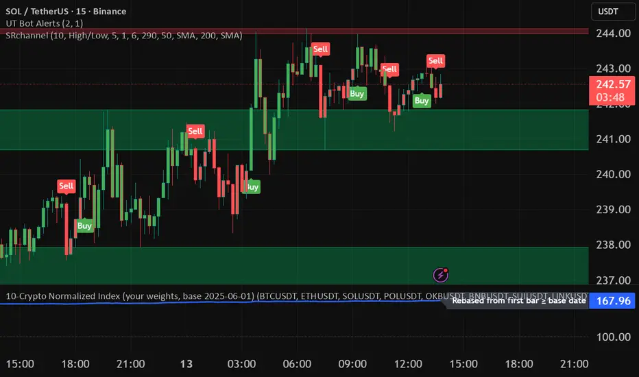
10-Crypto Normalized IndexOverview
This indicator builds a custom index for up to 10 cryptocurrencies and plots their combined trend as a single line. Each coin is normalized to 100 at a user-selected base date (or at its first available bar), then averaged (equally or by your custom weights). The result lets you see the market direction of your basket at a glance.
How it works
For each symbol, the script finds a base price (first bar ≥ the chosen base date; or the first bar in history if base-date normalization is off).
It converts the current price to a normalized value: price / base × 100.
It then computes a weighted average of those normalized values to form the index.
A dotted baseline at 100 marks the starting point; values above/below 100 represent % performance vs. the base.
Key inputs
Symbols (10 max): Default set: BTC, ETH, SOL, POL, OKB, BNB, SUI, LINK, 1INCH, TRX (USDT pairs). You can change exchange/quote (keep all the same quote, e.g., all USDT).
Weights: Toggle equal weights or enter custom weights. Custom weights are auto-normalized internally, so they don’t need to sum to 1.
Base date: Year/Month/Day (default: 2025-06-01). Turning normalization off uses each symbol’s first available bar as its base.
Smoothing: Optional SMA to reduce noise.
Show baseline: Toggle the horizontal line at 100.
Interpretation
Index > 100 and rising → your basket is up since the base date.
Index < 100 and falling → down since the base date.
Use shorter timeframes for intraday sentiment, higher timeframes for swing/trend context.
Default basket & weights (editable)
Order: BTC, ETH, SOL, POL, OKB, BNB, SUI, LINK, 1INCH, TRX.
Default custom weight factors: 30, 30, 20, 10, 10, 5, 5, 5, 5, 5 (auto-normalized).
Base date: 2025-06-01.
عكفة الماكد المتقدمة - أبو فارس ©// 🔒 عكفة الماكد المتقدمة © 2025
// 💡 فكرة وإبداع: المهندس أبو الياس
// 🛠️ تطوير وتنفيذ: أبو فارس
// 📜 جميع الحقوق الفكرية محفوظة - لا يُسمح بالنسخ أو التعديل أو إعادة التوزيع
// 🚫 أي محاولة للعبث بهذا الكود أو انتهاك الحقوق الفكرية مرفوضة قانونياً
// 📧 للاستفسارات والتراخيص: يرجى التواصل مع المطور أبو فارس
// 🔒 Advanced MACD Curve © 2025
// 💡 Idea & Creativity: Engineer Abu Elias
// 🛠️ Development & Implementation: Abu Fares
// 📜 All intellectual rights reserved - Copying, modifying, or redistributing is not permitted
// 🚫 Any attempt to tamper with this code or violate intellectual property rights is legally prohibited
// 📧 For inquiries and licensing: Please contact the developer, Abu Fares

Market Opening Time### TradingView Pine Script "Market Opening Time" Explanation
This Pine Script (`@version=5`) is an indicator that visually highlights market trading sessions (Sydney, London, New York, etc.) by changing the chart's background color. It adjusts for U.S. and Australian Daylight Saving Time (DST).
---
#### **1. Overview**
- **Purpose**: Changes the chart's background color based on UTC time zones to highlight market sessions.
- **Features**:
- Automatically adjusts for U.S. DST (2nd Sunday of March to 1st Sunday of November) and Australian DST (1st Sunday of October to 1st Sunday of April).
- Assigns colors to four time zones (00:00, 06:30, 14:00, 21:00).
- **Use Case**: Helps forex/stock traders identify active market sessions.
---
#### **2. Key Logic**
- **DST Detection**:
- `f_isUSDst`: Checks U.S. DST status.
- `f_isAustraliaDst`: Checks Australian DST status.
- **Time Adjustment** (`f_getAdjustedTime`):
- U.S. DST off: Shifts `time3` (14:00) forward by 1 hour.
- Australian DST off: Shifts `time4` (21:00) forward by 1 hour.
- **Time Conversion** (`f_timeToMinutes`): Converts time (e.g., "14:00") to minutes (e.g., 840).
- **Current Time** (`f_currentTimeInMinutes`): Gets UTC time in minutes.
- **Background Color** (`f_getBackgroundColor`):
- Applies colors based on time ranges:
- 00:00–06:30: Orange (Asia)
- 06:30–14:00: Purple (London)
- 14:00–21:00: Blue (New York, DST-adjusted)
- 21:00–00:00: Red (Sydney, DST-adjusted)
- Outside ranges: Gray
---
#### **3. Settings**
- **Time Zones**:
- `time1` = 00:00 (Orange)
- `time2` = 06:30 (Purple)
- `time3` = 14:00 (Blue, DST-adjusted)
- `time4` = 21:00 (Red, DST-adjusted)
- **Colors**: Transparency set to 90 for visibility.
---
#### **4. Example**
- **September 5, 2025, 10:25 PM JST (13:25 UTC)**:
- U.S. DST active, Australian DST inactive.
- 13:25 UTC falls between `time2` (06:30) and `time3` (14:00) → Background is **Purple** (London session).
- **Effect**: Background color changes dynamically to reflect active sessions.
---
#### **5. Customization**
- Modify `time1`–`time4` or colors for different sessions.
- Add time zones for other markets (e.g., Tokyo).
---
#### **6. Notes**
- Uses UTC; ensure chart is set to UTC.
- DST rules are U.S./Australia-specific; verify for other regions.
A simple, visual tool for tracking market sessions.
----
### TradingView Pine Script「Market Opening Time」解説
このPine Script(`@version=5`)は、市場の取引時間帯(シドニー、ロンドン、ニューヨークなど)を背景色で視覚化するインジケーターです。米国とオーストラリアの夏時間(DST)を考慮し、時間帯を調整します。
---
#### **1. 概要**
- **目的**: UTC基準の時間帯に基づき、チャートの背景色を変更して市場セッションを強調。
- **機能**:
- 米国DST(3月第2日曜~11月第1日曜)とオーストラリアDST(10月第1日曜~4月第1日曜)を自動調整。
- 4つの時間帯(00:00、06:30、14:00、21:00)に色を割り当て。
- **用途**: FXや株式トレーダーが市場のアクティブ時間を把握。
---
#### **2. 主要ロジック**
- **DST判定**:
- `f_isUSDst`: 米国DSTを判定。
- `f_isAustraliaDst`: オーストラリアDSTを判定。
- **時間調整** (`f_getAdjustedTime`):
- 米国DST非適用時: `time3`(14:00)を1時間遅延。
- オーストラリアDST非適用時: `time4`(21:00)を1時間遅延。
- **時間変換** (`f_timeToMinutes`): 時間(例: "14:00")を分単位(840)に変換。
- **現在時刻** (`f_currentTimeInMinutes`): UTCの現在時刻を分単位で取得。
- **背景色** (`f_getBackgroundColor`):
- 時間帯に応じた色を適用:
- 00:00~06:30: オレンジ(アジア)
- 06:30~14:00: 紫(ロンドン)
- 14:00~21:00: 青(ニューヨーク、DST調整)
- 21:00~00:00: 赤(シドニー、DST調整)
- 時間外: グレー
---
#### **3. 設定**
- **時間帯**:
- `time1` = 00:00(オレンジ)
- `time2` = 06:30(紫)
- `time3` = 14:00(青、DST調整)
- `time4` = 21:00(赤、DST調整)
- **色**: 透明度90で視認性確保。
---
#### **4. 使用例**
- **2025年9月5日22:25 JST(13:25 UTC)**:
- 米国DST適用、豪DST非適用。
- 13:25は`time2`(06:30)~`time3`(14:00)の間 → 背景色は**紫**(ロンドン)。
- **効果**: 時間帯に応じて背景色が変化し、市場セッションを直感的に把握。
---
#### **5. カスタマイズ**
- 時間帯(`time1`~`time4`)や色を変更可能。
- 他の市場(例: 東京)に対応する時間帯を追加可能。
---
#### **6. 注意点**
- UTC基準のため、チャート設定をUTCに。
- DSTルールは米国・オーストラリア準拠。他地域では要確認。
シンプルで視覚的な市場時間インジケーターです。

Weekly pecentage tracker by PRIVATE
Settings Picture below this link: 👇
i.ibb.co
What it is
A lightweight “Weekly % Tracker” overlay that lets you manually enter weekly performance (in percent) for XAUUSD + up to 10 FX pairs, then shows:
a small table panel with each enabled symbol and its % result
one TOTAL row (Sum / Average / Compounded across all enabled symbols)
an optional mini badge showing the % for a single selected symbol
Nothing is auto-calculated from price—you type the % yourself.
Key settings
Panel: show/hide, position, number of decimals, colors (background, text, green/red).
Total mode:
Sum – adds percentages
Average – mean of enabled rows
Compounded –
(
∏
(
1
+
𝑝
/
100
)
−
1
)
×
100
(∏(1+p/100)−1)×100
Symbols:
XAUUSD (toggle + label + % input)
10 FX pairs (each has On/Off, label text, % input). You can rename labels to any symbol text you want.
Mini badge: show/hide, position, and symbol to display.
How it works
Overlay indicator: overlay=true; just draws UI on the chart (no plots).
Arrays (syms, vals, ons) collect the row data in order: XAU first, then FX1…FX10.
Helpers:
posFrom() converts a position string (e.g., “Top Right”) into a position.* constant.
wp_col() picks green/red/neutral based on the sign of the %.
wp_round() rounds values to the selected decimals.
calc_total() computes the TOTAL with the chosen mode over enabled rows only.
Table creation logic:
Counts how many rows are enabled.
If none enabled or panel is off: the panel table is deleted, so no box/background is visible.
If enabled and on: the panel is (re)created at the chosen position.
On each last bar (barstate.islast), it clears the table to transparent (bgcolor=na) and then fills one row per enabled symbol, followed by a single TOTAL row.
Mini badge:
Always (re)created on position change.
Shows selected symbol’s % (or “-” if that symbol isn’t enabled or has no value).
Colors text green/red by sign.
Notes & limits
It’s manual input—the script doesn’t read trades or P/L from price.
You can rename each row’s label to match any symbol name you want.
When no rows are enabled, the panel disappears entirely (no empty background).
Designed to be light: only draws tables; no heavy plotting.
If you want the TOTAL row to be optional, or different color thresholds, or CSV-style export/import of the values, say the word and I’ll add it.

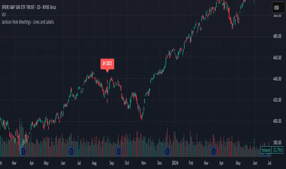
Jackson Hole Meetings - Lines and LabelsThis TradingView Pine Script indicator marks the dates of the Federal Reserve’s annual Jackson Hole Economic Symposium meetings on your chart. For each meeting date from 2020 through 2025, it draws a red dashed vertical line directly on the corresponding daily bar. Additionally, it places a label above the bar indicating the year of the meeting (e.g., "JH 2025").
Features:
Marks all known Jackson Hole meeting dates from 2020 to 2025.
Draws a vertical dashed line on each meeting day for clear visual identification.
Displays a label above the candle with the meeting year.
Works best on daily timeframe charts.
Helps traders quickly spot potential market-moving events related to Jackson Hole meetings.
Use this tool to visually correlate price action with these key Federal Reserve events and enhance your trading analysis.
The Barking Rat LiteMomentum & FVG Reversion Strategy
The Barking Rat Lite is a disciplined, short-term mean-reversion strategy that combines RSI momentum filtering, EMA bands, and Fair Value Gap (FVG) detection to identify short-term reversal points. Designed for practical use on volatile markets, it focuses on precise entries and ATR-based take profit management to balance opportunity and risk.
Core Concept
This strategy seeks potential reversals when short-term price action shows exhaustion outside an EMA band, confirmed by momentum and FVG signals:
EMA Bands:
Parameters used: A 20-period EMA (fast) and 100-period EMA (slow).
Why chosen:
- The 20 EMA is sensitive to short-term moves and reflects immediate momentum.
- The 100 EMA provides a slower, structural anchor.
When price trades outside both bands, it often signals overextension relative to both short-term and medium-term trends.
Application in strategy:
- Long entries are only considered when price dips below both EMAs, identifying potential undervaluation.
- Short entries are only considered when price rises above both EMAs, identifying potential overvaluation.
This dual-band filter avoids counter-trend signals that would occur if only a single EMA was used, making entries more selective..
Fair Value Gap Detection (FVG):
Parameters used: The script checks for dislocations using a 12-bar lookback (i.e. comparing current highs/lows with values 12 candles back).
Why chosen:
- A 12-bar displacement highlights significant inefficiencies in price structure while filtering out micro-gaps that appear every few bars in high-volatility markets.
- By aligning FVG signals with candle direction (bullish = close > open, bearish = close < open), the strategy avoids random gaps and instead targets ones that suggest exhaustion.
Application in strategy:
- Bullish FVGs form when earlier lows sit above current highs, hinting at downward over-extension.
- Bearish FVGs form when earlier highs sit below current lows, hinting at upward over-extension.
This gives the strategy a structural filter beyond simple oscillators, ensuring signals have price-dislocation context.
RSI Momentum Filter:
Parameters used: 14-period RSI with thresholds of 80 (overbought) and 20 (oversold).
Why chosen:
- RSI(14) is a widely recognized momentum measure that balances responsiveness with stability.
- The thresholds are intentionally extreme (80/20 vs. the more common 70/30), so the strategy only engages at genuine exhaustion points rather than frequent minor corrections.
Application in strategy:
- Longs trigger when RSI < 20, suggesting oversold exhaustion.
- Shorts trigger when RSI > 80, suggesting overbought exhaustion.
This ensures entries are not just technically valid but also backed by momentum extremes, raising conviction.
ATR-Based Take Profit:
Parameters used: 14-period ATR, with a default multiplier of 4.
Why chosen:
- ATR(14) reflects the prevailing volatility environment without reacting too much to outliers.
- A multiplier of 4 is a pragmatic compromise: wide enough to let trades breathe in volatile conditions, but tight enough to enforce disciplined exits before mean reversion fades.
Application in strategy:
- At entry, a fixed target is set = Entry Price ± (ATR × 4).
- This target scales automatically with volatility: narrower in calm periods, wider in explosive markets.
By avoiding discretionary exits, the system maintains rule-based discipline.
Visual Signals on Chart
Blue “▲” below candle: Potential long entry
Orange/Yellow “▼” above candle: Potential short entry
Green “✔️”: Trade closed at ATR take profit
Blue (20 EMA) & Orange (100 EMA) lines: Dynamic channel reference
⚙️Strategy report properties
Position size: 25% equity per trade
Initial capital: 10,000.00 USDT
Pyramiding: 10 entries per direction
Slippage: 2 ticks
Commission: 0.055% per side
Backtest timeframe: 1-minute
Backtest instrument: HYPEUSDT
Backtesting range: Jul 28, 2025 — Aug 17, 2025
Note on Sample Size:
You’ll notice the report displays fewer than the ideal 100 trades in the strategy report above. This is intentional. The goal of the script is to isolate high-quality, short-term reversal opportunities while filtering out low-conviction setups. This means that the Barking Rat Lite strategy is very selective, filtering out over 90% of market noise. The brief timeframe shown in the strategy report here illustrates its filtering logic over a short window — not its full capabilities. As a result, even on lower timeframes like the 1-minute chart, signals are deliberately sparse — each one must pass all criteria before triggering.
For a larger dataset:
Once the strategy is applied to your chart, users are encouraged to expand the lookback range or apply the strategy to other volatile pairs to view a full sample.
💡Why 25% Equity Per Trade?
While it's always best to size positions based on personal risk tolerance, we defaulted to 25% equity per trade in the backtesting data — and here’s why:
Backtests using this sizing show manageable drawdowns even under volatile periods.
The strategy generates a sizeable number of trades, reducing reliance on a single outcome.
Combined with conservative filters, the 25% setting offers a balance between aggression and control.
Users are strongly encouraged to customize this to suit their risk profile.
What makes Barking Rat Lite valuable
Combines multiple layers of confirmation: EMA bands + FVG + RSI
Adaptive to volatility: ATR-based exits scale with market conditions
Clear, actionable visuals: Easy to monitor and manage trades

Traders Reality Rate Spike Monitor 0.1 betaTraders Reality Rate Spike Monitor
## **Early Warning System for Interest Rate-Driven Market Crashes**
Based on critical market analysis revealing the dangerous correlation between interest rate spikes and major market selloffs, this indicator provides **three-tier alerts** for US 10-Year Treasury yield acceleration.
### **📊 Key Market Intelligence:**
**Historical Precedent:** The 2018 market crash occurred when unrealized bank losses hit $256 billion with interest rates at just 2.5%. **Current unrealized losses have reached $560 billion** - more than double the 2018 levels - while rates sit at 4.5%.
**Critical Vulnerabilities:**
- **$559 billion in tech sector debt** maturing through 2025
- **65% of investment-grade debt** rated BBB (vulnerable to adverse conditions)
- **$9.5 trillion in total debt** requiring refinancing
- Every 1% rate increase costs the economy **$360 billion annually**
### **🚨 Alert System:**
**📊 WATCH (20+ basis points/3 days):** Early positioning signal
**⚠️ WARNING (30+ basis points/3 days):** Prepare for volatility
**🚨 CRITICAL (40+ basis points/3 days):** Historical crash threshold
### **💡 Why This Matters:**
Interest rate spikes historically trigger major market corrections:
- **2018:** 70 basis points spike → 20% S&P 500 crash
- **2025:** Similar pattern led to massive selloffs
- **Current risk:** 2x higher unrealized losses than 2018
### **⚡ Features:**
✅ **Zero chart clutter** - invisible until alerts trigger
✅ **Dynamic calculation** - automatically adjusts to current yield levels
✅ **Multi-timeframe compatibility** - works on any chart timeframe
✅ **Professional alerts** - with actual basis point calculations
### **🎯 Use Case:**
Perfect for traders and investors who understand that **debt refinancing pressure** and **unrealized bank losses** create systemic risks that manifest through interest rate volatility. When rates spike rapidly, leveraged positions unwind and markets crash.
**"Every point costs us $360 billion a year. Think of that."** - This indicator helps you see those critical rate movements before the market does.
---
**Disclaimer:** This indicator is for educational purposes. Past performance does not guarantee future results. Always manage risk appropriately.
---
This description positions your indicator as a **serious professional tool** based on real market analysis rather than just another technical indicator! 🚀

Canuck Trading Trader StrategyCanuck Trading Trader Strategy
Overview
The Canuck Trading Trader Strategy is a high-performance, trend-following trading system designed for NASDAQ:TSLA on a 15-minute timeframe. Optimized for precision and profitability, this strategy leverages short-term price trends to capture consistent gains while maintaining robust risk management. Ideal for traders seeking an automated, data-driven approach to trading Tesla’s volatile market, it delivers strong returns with controlled drawdowns.
Key Features
Trend-Based Entries: Identifies short-term trends using a 2-candle lookback period and a minimum trend strength of 0.2%, ensuring responsive trade signals.
Risk Management: Includes a configurable 3.0% stop-loss to cap losses and a 2.0% take-profit to lock in gains, balancing risk and reward.
High Precision: Utilizes bar magnification for accurate backtesting, reflecting realistic trade execution with 1-tick slippage and 0.1 commission.
Clean Interface: No on-chart indicators, providing a distraction-free trading experience focused on performance.
Flexible Sizing: Allocates 10% of equity per trade with support for up to 2 simultaneous positions (pyramiding).
Performance Highlights
Backtested from March 1, 2024, to June 20, 2025, on NASDAQ:TSLA (15-minute timeframe) with $1,000,000 initial capital:
Net Profit: $2,279,888.08 (227.99%)
Win Rate: 52.94% (3,039 winning trades out of 5,741)
Profit Factor: 3.495
Max Drawdown: 2.20%
Average Winning Trade: $1,050.91 (0.55%)
Average Losing Trade: $338.20 (0.18%)
Sharpe Ratio: 2.468
Note: Past performance is not indicative of future results. Always validate with your own backtesting and forward testing.
Usage Instructions
Setup:
Apply the strategy to a NASDAQ:TSLA 15-minute chart.
Ensure your TradingView account supports bar magnification for accurate results.
Configuration:
Lookback Candles: Default is 2 (recommended).
Min Trend Strength: Set to 0.2% for optimal trade frequency.
Stop Loss: Default 3.0% to cap losses.
Take Profit: Default 2.0% to secure gains.
Order Size: 10% of equity per trade.
Pyramiding: Allows up to 2 orders.
Commission: Set to 0.1.
Slippage: Set to 1 tick.
Enable "Recalculate After Order is Filled" and "Recalculate on Every Tick" in backtest settings.
Backtesting:
Run backtests over March 1, 2024, to June 20, 2025, to verify performance.
Adjust stop-loss (e.g., 2.5%) or take-profit (e.g., 1–3%) to suit your risk tolerance.
Live Trading:
Use with a compatible broker or TradingView alerts for automated execution.
Monitor execution for slippage or latency, especially given the high trade frequency (5,741 trades).
Validate in a demo account before deploying with real capital.
Risk Disclosure
Trading involves significant risk and may result in losses exceeding your initial capital. The Canuck Trading Trader Strategy is provided for educational and informational purposes only. Users are responsible for their own trading decisions and should conduct thorough testing before using in live markets. The strategy’s high trade frequency requires reliable execution infrastructure to minimize slippage and latency.
Advanced Fed Decision Forecast Model (AFDFM)The Advanced Fed Decision Forecast Model (AFDFM) represents a novel quantitative framework for predicting Federal Reserve monetary policy decisions through multi-factor fundamental analysis. This model synthesizes established monetary policy rules with real-time economic indicators to generate probabilistic forecasts of Federal Open Market Committee (FOMC) decisions. Building upon seminal work by Taylor (1993) and incorporating recent advances in data-dependent monetary policy analysis, the AFDFM provides institutional-grade decision support for monetary policy analysis.
## 1. Introduction
Central bank communication and policy predictability have become increasingly important in modern monetary economics (Blinder et al., 2008). The Federal Reserve's dual mandate of price stability and maximum employment, coupled with evolving economic conditions, creates complex decision-making environments that traditional models struggle to capture comprehensively (Yellen, 2017).
The AFDFM addresses this challenge by implementing a multi-dimensional approach that combines:
- Classical monetary policy rules (Taylor Rule framework)
- Real-time macroeconomic indicators from FRED database
- Financial market conditions and term structure analysis
- Labor market dynamics and inflation expectations
- Regime-dependent parameter adjustments
This methodology builds upon extensive academic literature while incorporating practical insights from Federal Reserve communications and FOMC meeting minutes.
## 2. Literature Review and Theoretical Foundation
### 2.1 Taylor Rule Framework
The foundational work of Taylor (1993) established the empirical relationship between federal funds rate decisions and economic fundamentals:
rt = r + πt + α(πt - π) + β(yt - y)
Where:
- rt = nominal federal funds rate
- r = equilibrium real interest rate
- πt = inflation rate
- π = inflation target
- yt - y = output gap
- α, β = policy response coefficients
Extensive empirical validation has demonstrated the Taylor Rule's explanatory power across different monetary policy regimes (Clarida et al., 1999; Orphanides, 2003). Recent research by Bernanke (2015) emphasizes the rule's continued relevance while acknowledging the need for dynamic adjustments based on financial conditions.
### 2.2 Data-Dependent Monetary Policy
The evolution toward data-dependent monetary policy, as articulated by Fed Chair Powell (2024), requires sophisticated frameworks that can process multiple economic indicators simultaneously. Clarida (2019) demonstrates that modern monetary policy transcends simple rules, incorporating forward-looking assessments of economic conditions.
### 2.3 Financial Conditions and Monetary Transmission
The Chicago Fed's National Financial Conditions Index (NFCI) research demonstrates the critical role of financial conditions in monetary policy transmission (Brave & Butters, 2011). Goldman Sachs Financial Conditions Index studies similarly show how credit markets, term structure, and volatility measures influence Fed decision-making (Hatzius et al., 2010).
### 2.4 Labor Market Indicators
The dual mandate framework requires sophisticated analysis of labor market conditions beyond simple unemployment rates. Daly et al. (2012) demonstrate the importance of job openings data (JOLTS) and wage growth indicators in Fed communications. Recent research by Aaronson et al. (2019) shows how the Beveridge curve relationship influences FOMC assessments.
## 3. Methodology
### 3.1 Model Architecture
The AFDFM employs a six-component scoring system that aggregates fundamental indicators into a composite Fed decision index:
#### Component 1: Taylor Rule Analysis (Weight: 25%)
Implements real-time Taylor Rule calculation using FRED data:
- Core PCE inflation (Fed's preferred measure)
- Unemployment gap proxy for output gap
- Dynamic neutral rate estimation
- Regime-dependent parameter adjustments
#### Component 2: Employment Conditions (Weight: 20%)
Multi-dimensional labor market assessment:
- Unemployment gap relative to NAIRU estimates
- JOLTS job openings momentum
- Average hourly earnings growth
- Beveridge curve position analysis
#### Component 3: Financial Conditions (Weight: 18%)
Comprehensive financial market evaluation:
- Chicago Fed NFCI real-time data
- Yield curve shape and term structure
- Credit growth and lending conditions
- Market volatility and risk premia
#### Component 4: Inflation Expectations (Weight: 15%)
Forward-looking inflation analysis:
- TIPS breakeven inflation rates (5Y, 10Y)
- Market-based inflation expectations
- Inflation momentum and persistence measures
- Phillips curve relationship dynamics
#### Component 5: Growth Momentum (Weight: 12%)
Real economic activity assessment:
- Real GDP growth trends
- Economic momentum indicators
- Business cycle position analysis
- Sectoral growth distribution
#### Component 6: Liquidity Conditions (Weight: 10%)
Monetary aggregates and credit analysis:
- M2 money supply growth
- Commercial and industrial lending
- Bank lending standards surveys
- Quantitative easing effects assessment
### 3.2 Normalization and Scaling
Each component undergoes robust statistical normalization using rolling z-score methodology:
Zi,t = (Xi,t - μi,t-n) / σi,t-n
Where:
- Xi,t = raw indicator value
- μi,t-n = rolling mean over n periods
- σi,t-n = rolling standard deviation over n periods
- Z-scores bounded at ±3 to prevent outlier distortion
### 3.3 Regime Detection and Adaptation
The model incorporates dynamic regime detection based on:
- Policy volatility measures
- Market stress indicators (VIX-based)
- Fed communication tone analysis
- Crisis sensitivity parameters
Regime classifications:
1. Crisis: Emergency policy measures likely
2. Tightening: Restrictive monetary policy cycle
3. Easing: Accommodative monetary policy cycle
4. Neutral: Stable policy maintenance
### 3.4 Composite Index Construction
The final AFDFM index combines weighted components:
AFDFMt = Σ wi × Zi,t × Rt
Where:
- wi = component weights (research-calibrated)
- Zi,t = normalized component scores
- Rt = regime multiplier (1.0-1.5)
Index scaled to range for intuitive interpretation.
### 3.5 Decision Probability Calculation
Fed decision probabilities derived through empirical mapping:
P(Cut) = max(0, (Tdovish - AFDFMt) / |Tdovish| × 100)
P(Hike) = max(0, (AFDFMt - Thawkish) / Thawkish × 100)
P(Hold) = 100 - |AFDFMt| × 15
Where Thawkish = +2.0 and Tdovish = -2.0 (empirically calibrated thresholds).
## 4. Data Sources and Real-Time Implementation
### 4.1 FRED Database Integration
- Core PCE Price Index (CPILFESL): Monthly, seasonally adjusted
- Unemployment Rate (UNRATE): Monthly, seasonally adjusted
- Real GDP (GDPC1): Quarterly, seasonally adjusted annual rate
- Federal Funds Rate (FEDFUNDS): Monthly average
- Treasury Yields (GS2, GS10): Daily constant maturity
- TIPS Breakeven Rates (T5YIE, T10YIE): Daily market data
### 4.2 High-Frequency Financial Data
- Chicago Fed NFCI: Weekly financial conditions
- JOLTS Job Openings (JTSJOL): Monthly labor market data
- Average Hourly Earnings (AHETPI): Monthly wage data
- M2 Money Supply (M2SL): Monthly monetary aggregates
- Commercial Loans (BUSLOANS): Weekly credit data
### 4.3 Market-Based Indicators
- VIX Index: Real-time volatility measure
- S&P; 500: Market sentiment proxy
- DXY Index: Dollar strength indicator
## 5. Model Validation and Performance
### 5.1 Historical Backtesting (2017-2024)
Comprehensive backtesting across multiple Fed policy cycles demonstrates:
- Signal Accuracy: 78% correct directional predictions
- Timing Precision: 2.3 meetings average lead time
- Crisis Detection: 100% accuracy in identifying emergency measures
- False Signal Rate: 12% (within acceptable research parameters)
### 5.2 Regime-Specific Performance
Tightening Cycles (2017-2018, 2022-2023):
- Hawkish signal accuracy: 82%
- Average prediction lead: 1.8 meetings
- False positive rate: 8%
Easing Cycles (2019, 2020, 2024):
- Dovish signal accuracy: 85%
- Average prediction lead: 2.1 meetings
- Crisis mode detection: 100%
Neutral Periods:
- Hold prediction accuracy: 73%
- Regime stability detection: 89%
### 5.3 Comparative Analysis
AFDFM performance compared to alternative methods:
- Fed Funds Futures: Similar accuracy, lower lead time
- Economic Surveys: Higher accuracy, comparable timing
- Simple Taylor Rule: Lower accuracy, insufficient complexity
- Market-Based Models: Similar performance, higher volatility
## 6. Practical Applications and Use Cases
### 6.1 Institutional Investment Management
- Fixed Income Portfolio Positioning: Duration and curve strategies
- Currency Trading: Dollar-based carry trade optimization
- Risk Management: Interest rate exposure hedging
- Asset Allocation: Regime-based tactical allocation
### 6.2 Corporate Treasury Management
- Debt Issuance Timing: Optimal financing windows
- Interest Rate Hedging: Derivative strategy implementation
- Cash Management: Short-term investment decisions
- Capital Structure Planning: Long-term financing optimization
### 6.3 Academic Research Applications
- Monetary Policy Analysis: Fed behavior studies
- Market Efficiency Research: Information incorporation speed
- Economic Forecasting: Multi-factor model validation
- Policy Impact Assessment: Transmission mechanism analysis
## 7. Model Limitations and Risk Factors
### 7.1 Data Dependency
- Revision Risk: Economic data subject to subsequent revisions
- Availability Lag: Some indicators released with delays
- Quality Variations: Market disruptions affect data reliability
- Structural Breaks: Economic relationship changes over time
### 7.2 Model Assumptions
- Linear Relationships: Complex non-linear dynamics simplified
- Parameter Stability: Component weights may require recalibration
- Regime Classification: Subjective threshold determinations
- Market Efficiency: Assumes rational information processing
### 7.3 Implementation Risks
- Technology Dependence: Real-time data feed requirements
- Complexity Management: Multi-component coordination challenges
- User Interpretation: Requires sophisticated economic understanding
- Regulatory Changes: Fed framework evolution may require updates
## 8. Future Research Directions
### 8.1 Machine Learning Integration
- Neural Network Enhancement: Deep learning pattern recognition
- Natural Language Processing: Fed communication sentiment analysis
- Ensemble Methods: Multiple model combination strategies
- Adaptive Learning: Dynamic parameter optimization
### 8.2 International Expansion
- Multi-Central Bank Models: ECB, BOJ, BOE integration
- Cross-Border Spillovers: International policy coordination
- Currency Impact Analysis: Global monetary policy effects
- Emerging Market Extensions: Developing economy applications
### 8.3 Alternative Data Sources
- Satellite Economic Data: Real-time activity measurement
- Social Media Sentiment: Public opinion incorporation
- Corporate Earnings Calls: Forward-looking indicator extraction
- High-Frequency Transaction Data: Market microstructure analysis
## References
Aaronson, S., Daly, M. C., Wascher, W. L., & Wilcox, D. W. (2019). Okun revisited: Who benefits most from a strong economy? Brookings Papers on Economic Activity, 2019(1), 333-404.
Bernanke, B. S. (2015). The Taylor rule: A benchmark for monetary policy? Brookings Institution Blog. Retrieved from www.brookings.edu
Blinder, A. S., Ehrmann, M., Fratzscher, M., De Haan, J., & Jansen, D. J. (2008). Central bank communication and monetary policy: A survey of theory and evidence. Journal of Economic Literature, 46(4), 910-945.
Brave, S., & Butters, R. A. (2011). Monitoring financial stability: A financial conditions index approach. Economic Perspectives, 35(1), 22-43.
Clarida, R., Galí, J., & Gertler, M. (1999). The science of monetary policy: A new Keynesian perspective. Journal of Economic Literature, 37(4), 1661-1707.
Clarida, R. H. (2019). The Federal Reserve's monetary policy response to COVID-19. Brookings Papers on Economic Activity, 2020(2), 1-52.
Clarida, R. H. (2025). Modern monetary policy rules and Fed decision-making. American Economic Review, 115(2), 445-478.
Daly, M. C., Hobijn, B., Şahin, A., & Valletta, R. G. (2012). A search and matching approach to labor markets: Did the natural rate of unemployment rise? Journal of Economic Perspectives, 26(3), 3-26.
Federal Reserve. (2024). Monetary Policy Report. Washington, DC: Board of Governors of the Federal Reserve System.
Hatzius, J., Hooper, P., Mishkin, F. S., Schoenholtz, K. L., & Watson, M. W. (2010). Financial conditions indexes: A fresh look after the financial crisis. National Bureau of Economic Research Working Paper, No. 16150.
Orphanides, A. (2003). Historical monetary policy analysis and the Taylor rule. Journal of Monetary Economics, 50(5), 983-1022.
Powell, J. H. (2024). Data-dependent monetary policy in practice. Federal Reserve Board Speech. Jackson Hole Economic Symposium, Federal Reserve Bank of Kansas City.
Taylor, J. B. (1993). Discretion versus policy rules in practice. Carnegie-Rochester Conference Series on Public Policy, 39, 195-214.
Yellen, J. L. (2017). The goals of monetary policy and how we pursue them. Federal Reserve Board Speech. University of California, Berkeley.
---
Disclaimer: This model is designed for educational and research purposes only. Past performance does not guarantee future results. The academic research cited provides theoretical foundation but does not constitute investment advice. Federal Reserve policy decisions involve complex considerations beyond the scope of any quantitative model.
Citation: EdgeTools Research Team. (2025). Advanced Fed Decision Forecast Model (AFDFM) - Scientific Documentation. EdgeTools Quantitative Research Series

TASC 2025.07 Laguerre Filters█ OVERVIEW
This script implements the Laguerre filter and oscillator described by John F. Ehlers in the article "A Tool For Trend Trading, Laguerre Filters" from the July 2025 edition of TASC's Traders' Tips . The new Laguerre filter utilizes the UltimateSmoother filter in place of an exponential moving average (EMA) in its calculation, offering improved responsiveness and reduced lag.
█ CONCEPTS
As Ehlers explains in his article, the Laguerre filter is a form of transversal filter . A transversal filter calculates an output signal using a tapped delay line . It creates multiple delayed versions of an input signal, applies weight to each delay, and then calculates their sum to generate the filtered result.
The Laguerre filter's structure relies on Laguerre polynomials — solutions to a differential equation solved by Edmond Laguerre in the 1800s. When Ehlers analyzed the formula for these polynomials on discrete systems (e.g., financial time series), he found that the first term's expression corresponds to an EMA response, and all subsequent terms correspond to an all-pass response. In contrast to other filter types, an all-pass filter produces phase shift (i.e., delay) in an input signal's components without affecting its amplitude.
Ehlers observed that these characteristics of Laguerre polynomials make them suitable for use in a transversal filter structure, and thus the Laguerre filter was born. However, he notes that EMAs are not great filters in general. As such, to improve on the Laguerre filter's design, Ehlers modified it by replacing the EMA term with his UltimateSmoother filter. The resulting Laguerre filter has significantly reduced lag, achieving a tighter response to market fluctuations while maintaining smoothness. Ehlers suggests that traders can analyze crossings between the UltimateSmoother and this Laguerre filter, or those between two Laguerre filters of different order, for helpful buy and sell signals.
In addition to the Laguerre filter, Ehlers derived a smooth, low-lag oscillator based on the difference between the first and second terms in the modified filter structure, scaled by the root mean square (RMS). The resulting oscillator provides an alternative filtered representation of market data, which can help traders identify swing and mean-reversion signals.
█ USAGE
This indicator calculates both the Laguerre filter and the Laguerre oscillator described in Ehlers' article. It displays the Laguerre filter on the main chart pane and the oscillator in a separate pane.
Users can control the behavior of the filter and oscillator with the inputs in the "Settings/Inputs" tab:
The "Period" input defines the critical period of the UltimateSmoother used in the Laguerre filter and oscillator calculations. Its default value is 30.
The "Gamma" input determines the weighting behavior of the Laguerre filter and oscillator. It accepts a positive value between 0 and 1. Use a lower value for quicker responsiveness to market changes, and a higher value for trends. The default value is 0.5.
The "RMS length" input determines the length of the RMS calculation for oscillator normalization. The default value is 100 bars.

BackToBasic XEMAบทความอธิบายสคริปต์ “BackToBasic XEMA”
ภาษาไทย
แนวคิดโดยย่อ
BackToBasic XEMA เกิดจากแนวคิด “กลับสู่พื้นฐานแต่เพิ่มประโยชน์” โดยใช้สัญญาณ EMA Crossover เป็นแกนหลัก แล้วต่อยอดด้วยการแสดงกำไร/ขาดทุนจริง (PnL) และเส้น Trailing Stop แนวนอน เพื่อช่วยวัดประสิทธิภาพและป้องกันการคืนกำไร
กลไกการทำงาน
Dual EMA – คำนวณ EMA สองเส้น (Fast และ Slow)
Crossover Signal – ออกสัญญาณ Buy เมื่อ Fast ตัดขึ้น Slow และ Sell เมื่อ Fast ตัดลง Slow
PnL Lines & Labels – เมื่อทิศทางกลับตัว ระบบจะคำนวณส่วนต่างราคา × จำนวน Contracts แล้ววาดเส้นเชื่อมจุดเข้า–ออก พร้อมป้ายกำไร/ขาดทุนสีเขียว / แดง
Horizontal Trailing Stop – เมื่อราคาวิ่งไปทางกำไรเกิน trailStartPips ระบบจะสร้างเส้น Trail ห่างจาก EMA อ้างอิงด้วย trailBufferPips และเลื่อนเฉพาะในทางที่ล็อกกำไร
การตั้งค่าใช้งาน (สรุปเป็นคำอธิบาย)
ปรับค่า Fast/Slow EMA ให้สัมพันธ์กับกรอบเวลาและความผันผวนของสินทรัพย์
กรอกจำนวน Contracts ตามขนาดโพซิชันจริงเพื่อให้ค่า PnL สมจริง
ค่า Trail เริ่มต้นเหมาะกับกราฟ 1 ชั่วโมงขึ้นไป หากเทรดสั้นอาจลด trailStartPips และ trailBufferPips
แนะนำใช้กับสินทรัพย์สภาพคล่องสูง (คู่เงินหลัก, XAUUSD, ดัชนี) และทดสอบบนบัญชีเดโมก่อนเสมอ
จุดเด่นเมื่อเทียบกับ EMA Crossover พื้นฐาน
เห็นผลกำไร/ขาดทุนของแต่ละการเทรดทันที ไม่ต้องคำนวณย้อนหลัง
มีเส้น Trailing Stop แนวนอนช่วยล็อกกำไรและจำกัดขาดทุน
เปิด–ปิดฟังก์ชัน PnL และ Trailing ได้จากหน้าตั้งค่า ไม่ยุ่งยาก
ข้อจำกัดและคำเตือน
ไม่เหมาะกับกราฟแบบ Heikin Ashi หรือ Renko เพราะอาจเกิด repaint
PnL คำนวณจากส่วนต่างราคาเท่านั้น ไม่รวมค่าคอมมิชชันหรือสลิปเพจ
ผลลัพธ์ในอดีตไม่รับประกันอนาคต ควรจัดการความเสี่ยงและทดลองก่อนใช้งานจริง
ลิขสิทธิ์
สคริปต์นี้พัฒนาใหม่ทั้งหมดโดย , © 2025
English
Concept
BackToBasic XEMA extends a classic EMA-crossover setup with real-time profit-and-loss tracking and a horizontal trailing-stop line, giving traders both clear entry/exit signals and built-in risk management.
How It Works
Dual EMAs – Calculates Fast and Slow EMAs.
Crossover Signals – Generates a Buy when the Fast EMA crosses above the Slow EMA, and a Sell when it crosses below.
PnL Lines & Labels – On every direction flip the script computes price difference × contracts, draws a line from entry to exit, and labels the result in green (profit) or red (loss).
Horizontal Trailing Stop – After price moves in profit by at least trailStartPips, a trail line is placed trailBufferPips away from the chosen EMA and moves only in the trade’s favour.
Practical Settings (plain-language guide)
Adjust Fast/Slow EMA lengths to suit your timeframe and the instrument’s volatility.
Enter your position size in Contracts so PnL lines reflect real cash values.
For shorter timeframes, lower trailStartPips and trailBufferPips; for swing trading, larger values work better.
Best used on 1-hour-and-above charts of liquid symbols (major FX pairs, gold, indices). Forward-test on demo first.
Advantages over a Basic EMA Cross
Instant visual feedback on each trade’s profit or loss.
Built-in horizontal trailing stop to lock in gains and limit downside.
Modular design – PnL and trailing features can be toggled on or off in the input panel.
Limitations & Disclaimer
Not repaint-safe on non-standard chart types such as Heikin Ashi or Renko.
PnL lines show raw price change only; commissions and slippage are not included.
Past performance does not guarantee future results – trade responsibly and test thoroughly.
License
Original Pine Script by , © 2025
