Filtered MACD with Backtest [UAlgo]The "Filtered MACD with Backtest " indicator is an advanced trading tool designed for the TradingView platform. It combines the Moving Average Convergence Divergence (MACD) with additional filters such as Moving Average (MA) and Average Directional Index (ADX) to enhance trading signals. This indicator aims to provide more reliable entry and exit points by filtering out noise and confirming trends. Additionally, it includes a comprehensive backtesting module to simulate trading strategies and assess their performance based on historical data. The visual backtest module allows traders to see potential trades directly on the chart, making it easier to evaluate the effectiveness of the strategy.
🔶 Customizable Parameters :
Price Source Selection: Users can choose their preferred price source for calculations, providing flexibility in analysis.
Filter Parameters:
MA Filter: Option to use a Moving Average filter with types such as EMA, SMA, WMA, RMA, and VWMA, and a customizable length.
ADX Filter: Option to use an ADX filter with adjustable length and threshold to determine trend strength.
MACD Parameters: Customizable fast length, slow length, and signal smoothing for the MACD indicator.
Backtest Module:
Entry Type: Supports "Buy and Sell", "Buy", and "Sell" strategies.
Stop Loss Types: Choose from ATR-based, fixed point, or X bar high/low stop loss methods.
Reward to Risk Ratio: Set the desired take profit level relative to the stop loss.
Backtest Visuals: Display entry, stop loss, and take profit levels directly on the chart with
colored backgrounds.
Alerts: Configurable alerts for buy and sell signals.
🔶 Filtered MACD : Understanding How Filters Work with ADX and MA
ADX Filter:
The Average Directional Index (ADX) measures the strength of a trend. The script calculates ADX using the user-defined length and applies a threshold value.
Trading Signals with ADX Filter:
Buy Signal: A regular MACD buy signal (crossover of MACD line above the signal line) is only considered valid if the ADX is above the set threshold. This suggests a stronger uptrend to potentially capitalize on.
Sell Signal: Conversely, a regular MACD sell signal (crossunder of MACD line below the signal line) is only considered valid if the ADX is above the threshold, indicating a stronger downtrend for potential shorting opportunities.
Benefits: The ADX filter helps avoid whipsaws or false signals that might occur during choppy market conditions with weak trends.
MA Filter:
You can choose from various Moving Average (MA) types (EMA, SMA, WMA, RMA, VWMA) for the filter. The script calculates the chosen MA based on the user-defined length.
Trading Signals with MA Filter:
Buy Signal: A regular MACD buy signal is only considered valid if the closing price is above the MA value. This suggests a potential uptrend confirmed by the price action staying above the moving average.
Sell Signal: Conversely, a regular MACD sell signal is only considered valid if the closing price is below the MA value. This suggests a potential downtrend confirmed by the price action staying below the moving average.
Benefits: The MA filter helps identify potential trend continuation opportunities by ensuring the price aligns with the chosen moving average direction.
Combining Filters:
You can choose to use either the ADX filter, the MA filter, or both depending on your strategy preference. Using both filters adds an extra layer of confirmation for your signals.
🔶 Backtesting Module
The backtesting module in this script allows you to visually assess how the filtered MACD strategy would have performed on historical data. Here's a deeper dive into its features:
Backtesting Type: You can choose to backtest for buy signals only, sell signals only, or both. This allows you to analyze the strategy's effectiveness in different market conditions.
Stop-Loss Types: You can define how stop-loss orders are placed:
ATR (Average True Range): This uses a volatility measure (ATR) multiplied by a user-defined factor to set the stop-loss level.
Fixed Point: This allows you to specify a fixed dollar amount or percentage value as the stop-loss.
X bar High/Low: This sets the stop-loss at a certain number of bars (defined by the user) above/below the bar's high (for long positions) or low (for short positions).
Reward-to-Risk Ratio: Define the desired ratio between your potential profit and potential loss on each trade. The backtesting module will calculate take-profit levels based on this ratio and the stop-loss placement.
🔶 Disclaimer:
Use with Caution: This indicator is provided for educational and informational purposes only and should not be considered as financial advice. Users should exercise caution and perform their own analysis before making trading decisions based on the indicator's signals.
Not Financial Advice: The information provided by this indicator does not constitute financial advice, and the creator (UAlgo) shall not be held responsible for any trading losses incurred as a result of using this indicator.
Backtesting Recommended: Traders are encouraged to backtest the indicator thoroughly on historical data before using it in live trading to assess its performance and suitability for their trading strategies.
Risk Management: Trading involves inherent risks, and users should implement proper risk management strategies, including but not limited to stop-loss orders and position sizing, to mitigate potential losses.
No Guarantees: The accuracy and reliability of the indicator's signals cannot be guaranteed, as they are based on historical price data and past performance may not be indicative of future results.
Backtest

MetaFOX DCA (ASAP-RSI-BB%B-TV)Welcome To ' MetaFOX DCA (ASAP-RSI-BB%B-TV) ' Indicator.
This is not a Buy/Sell signals indicator, this is an indicator to help you create your own strategy using a variety of technical analyzing options within the indicator settings with the ability to do DCA (Dollar Cost Average) with up to 100 safety orders.
It is important when backtesting to get a real results, but this is impossible, especially when the time frame is large, because we don't know the real price action inside each candle, as we don't know whether the price reached the high or low first. but what I can say is that I present to you a backtest results in the worst possible case, meaning that if the same chart is repeated during the next period and you traded for the same period and with the same settings, the real results will be either identical to the results in the indicator or better (not worst). There will be no other factors except the slippage in the price when executing orders in the real trading, So I created a feature for that to increase the accuracy rate of the results. For more information, read this description.
Below I will explain all the properties and settings of the indicator:
A) 'Buy Strategies' Section: Your choices of strategies to Start a new trade: (All the conditions works as (And) not (OR), You have to choose one at least and you can choose more than one).
- 'ASAP (New Candle)': Start a trade as soon as possible at the opening of a new candle after exiting the previous trade.
- 'RSI': Using RSI as a technical analysis condition to start a trade.
- 'BB %B': Using BB %B as a technical analysis condition to start a trade.
- 'TV': Using tradingview crypto screener as a technical analysis condition to start a trade.
B) 'Exit Strategies' Section: Your choices of strategies to Exit the trades: (All the conditions works as (And) not (OR), You can choose more than one, But if you don't want to use any of them you have to activate the 'Use TP:' at least).
- 'ASAP (New Candle)': Exit a trade as soon as possible at the opening of a new candle after opening the previous trade.
- 'RSI': Using RSI as a technical analysis condition to exit a trade.
- 'BB %B': Using BB %B as a technical analysis condition to exit a trade.
- 'TV': Using tradingview crypto screener as a technical analysis condition to exit a trade.
C) 'Main Settings' Section:
- 'Trading Fees %': The Exchange trading fees in percentage (trading Commission).
- 'Entry Price Slippage %': Since real trading differs from backtest calculations, while in backtest results are calculated based on the open price of the candle, but in real trading there is a slippage from the open price of the candle resulting from the supply and demand in the real time trading, so this feature is to determine the slippage Which you think it is appropriate, then the entry prices of the trades will calculated higher than the open price of the start candle by the percentage of slippage that you set. If you don't want to calculate any slippage, just set it to zero, but I don't recommend that if you want the most realistic results.
Note: If (open price + slippage) is higher than the high of the candle then don't worry, I've kept this in consideration.
- 'Use SL': Activate to use stop loss percentage.
- 'SL %': Stop loss percentage.
- 'SL settings options box':
'SL From Base Price': Calculate the SL from the base order price (from the trade first entry price).
'SL From Avg. Price': Calculate the SL from the average price in case you use safety orders.
'SL From Last SO.': Calculate the SL from the last (lowest) safety order deviation.
ex: If you choose 'SL From Avg. Price' and SL% is 5, then the SL will be lower than the average price by 5% (in this case your SL will be dynamic until the price reaches all the safety orders unlike the other two SL options).
Note: This indicator programmed to be compatible with '3COMMAS' platform, but I added more options that came to my mind.
'3COMMAS' DCA bots uses 'SL From Base Price'.
- 'Use TP': Activate to use take profit percentage.
- 'TP %': Take profit percentage.
- 'Pure TP,SL': This feature was created due to the differences in the method of calculations between API tools trading platforms:
If the feature is not activated and (for example) the TP is 5%, this means that the price must move upward by only 5%, but you will not achieve a net profit of 5% due to the trading fees. but If the feature is activated, this means that you will get a net profit of 5%, and this means that the price must move upward by (5% for the TP + the equivalent of trading fees). The same idea is applied to the SL.
Note: '3COMMAS' DCA bots uses activated 'Pure TP,SL'.
- 'SO. Price Deviation %': Determines the decline percentage for the first safety order from the trade start entry price.
- 'SO. Step Scale': Determines the deviation multiplier for the safety orders.
Note: I'm using the same method of calculations for SO. (safety orders) levels that '3COMMAS' platform is using. If there is any difference between the '3COMMAS' calculations and the platform that you are using, please let me know.
'3COMMAS' DCA bots minimum 'SO. Price Deviation %' is (0.21)
'3COMMAS' DCA bots minimum 'SO. Step Scale' is (0.1)
- 'SO. Volume Scale': Determines the base order size multiplier for the safety orders sizes.
ex: If you used 10$ to buy at the trade start (base order size) and your 'SO. Volume Scale' is 2, then the 1st SO. size will be 20, the 2nd SO. size will be 40 and so on.
- 'SO. Count': Determines the number of safety orders that you want. If you want to trade without safety orders set it to zero.
'3COMMAS' DCA bots minimum 'SO. Volume Scale' is (0.1)
- 'Exchange Min. Size': The exchange minimum size per trade, It's important to prevent you from setting the base order Size less than the exchange limit. It's also important for the backtest results calculations.
ex: If you setup your strategy settings and it led to a loss to the point that you can't trade any more due to insufficient funds and your base order size share from the strategy becomes less than the exchange minimum trade size, then the indicator will show you a warning and will show you the point where you stopped the trading (It works in compatible with the initial capital). I recommend to set it a little bit higher than the real exchange minimum trade size especially if you trade without safety orders to not stuck in the trade if you hit the stop loss
- 'BO. Size': The base order size (funds you use at the trade entry).
- 'Initial Capital': The total funds allocated for trading using your strategy settings, It can be more than what is required in the strategy to cover the deficit in case of a loss, but it should not exceed the funds that you actually have for trading using this strategy settings, It's important to prevent you from setting up a strategy which requires funds more than what you have. It's also has other important benefits (refer to 'Exchange Min. Size' for more information).
- 'Accumulative Results': This feature is also called re-invest profits & risk reduction. If it's not activated then you will use the same funds size in each new trade whether you are in profit or loss till the (initial capitals + net results) turns insufficient. If it's activated then you will reuse your profits and losses in each new trade.
ex: The feature is active and your first trade ended with a net profit of 1000$, the next trade will add the 1000$ to the trade funds size and it will be distributed as a percentage to the BO. & SO.s according to your strategy settings. The same idea in case of a loss, the trade funds size will be reduced.
D) 'RSI Strategy' Section:
- 'Buy': RSI technical condition to start a trade. Has no effect if you don't choose 'RSI' option in 'Buy Strategies'.
- 'Exit': RSI technical condition to exit a trade. Has no effect if you don't choose 'RSI' option in 'Exit Strategies'.
E) 'TV Strategy' Section:
- 'Buy': TradingView Crypto Screener technical condition to start a trade. Has no effect if you don't choose 'TV' option in 'Buy Strategies'.
- 'Exit': TradingView Crypto Screener technical condition to exit a trade. Has no effect if you don't choose 'TV' option in 'Exit Strategies'.
F) 'BB %B Strategy' Section:
- 'Buy': BB %B technical condition to start a trade. Has no effect if you don't choose 'BB %B' option in 'Buy Strategies'.
- 'Exit': BB %B technical condition to exit a trade. Has no effect if you don't choose 'BB %B' option in 'Exit Strategies'.
G) 'Plot' Section:
- 'Signals': Plots buy and exit signals.
- 'BO': Plots the trade entry price (base order price).
- 'AVG': Plots the trade average price.
- 'AVG options box': Your choice to plot the trade average price type:
'Avg. With Fees': The trade average price including the trading fees, If you exit the trade at this price the trade net profit will be 0.00
'Avg. Without Fees': The trade average price but not including the trading fees, If you exit the trade at this price the trade net profit will be a loss equivalent to the trading fees.
- 'TP': Plots the trade take profit price.
- 'SL': Plots the trade stop loss price.
- 'Last SO': Plots the trade last safety order that the price reached.
- 'Exit Price': Plots a mark on the trade exit price, It plots in 3 colors as below:
Red (Default): Trade exit at a loss.
Green (Default): Trade exit at a profit.
Yellow (Default): Trade exit at a profit but this is a special case where we have to calculate the profits before reaching the safety orders (if any) on that candle (compatible with the idea of getting strategy results at the worst case).
- 'Result Table': Plots your strategy result table. The net profit percentage shown is a percentage of the 'initial capital'.
- 'TA Values': Plots your used strategies Technical analysis values. (Green cells means valid condition).
- 'Help Table': Plots a table to help you discover 100 safety orders with its deviations and the total funds needed for your strategy settings. Deviations shown in red is impossible to use because its price is <= 0.00
- 'Portfolio Chart': Plots your Portfolio status during the entire trading period in addition to the highest and lowest level reached. It's important when evaluating any strategy not only to look at the final result, but also to look at the change in results over the entire trading period. Perhaps the results were worryingly negative at some point before they rose again and made a profit. This feature helps you to see the whole picture.
- 'Welcome Message': Plots a welcome message and showing you the idea behind this indicator.
- 'Green Net Profit %': It plots the 'Net Profit %' in the result table in green color if the result is equal to or above the value that you entered.
- 'Green Win Rate %': It plots the 'Win Rate %' in the result table in green color if the result is equal to or above the value that you entered.
- 'User Notes Area': An empty text area, Feel free to use this area to write your notes so you don't forget them.
The indicator will take care of you. In some cases, warning messages will appear for you. Read them carefully, as they mean that you have done an illogical error in the indicator settings. Also, the indicator will sometimes stop working for the same reason mentioned above. If that happens then click on the red (!) next to the indicator name and read the message to find out what illogical error you have done.
Please enjoy the indicator and let me know your thoughts in the comments below.

GKD-BT Optimizer SCSC Backtest [Loxx]The Giga Kaleidoscope GKD-BT Optimizer SCSC Backtest (Solo Confirmation Super Complex) is a Backtest module included in AlgxTrading's "Giga Kaleidoscope Modularized Trading System." (see the section Giga Kaleidoscope (GKD) Modularized Trading System below for an explanation of the GKD trading system)
**the backtest data rendered to the chart above and all screenshots below use $5 commission per trade and 10% equity per trade with $1 million initial capital**
█ GKD-BT Optimizer SCSC Backtest
The GKD-BT Optimizer SCSC Backtest is a comprehensive backtesting module designed to optimize the combination of key GKD indicators within AlgxTrading's "Giga Kaleidoscope Modularized Trading System." This module facilitates precise strategy refinement by allowing traders to configure and optimize the following critical GKD indicators:
GKD-B Baseline
GKD-V Volatility/Volume
GKD-C Confirmation 1
GKD-C Continuation
Each indicator is equipped with an "Optimizer" mode, enabling dynamic feedback and iterative improvements directly into the backtesting environment. This integrated approach ensures that each component contributes effectively to the overall strategy, providing a robust framework for achieving optimized trading outcomes.
The GKD-BT Optimizer supports granular test configurations including a single take profit and stop loss setting, and allows for targeted testing within specified date ranges to simulate forward testing with historical data. This feature is essential for evaluating the resilience and effectiveness of trading strategies under various market conditions.
Furthermore, the module is designed with user-centric features such as:
Customizable Trading Panel: Displays critical backtest results and trade statistics, which can be shown or hidden as per user preference.
Highlighting Thresholds: Users can set thresholds for Total Percent Wins, Percent Profitable, and Profit Factor, which helps in quickly identifying the most relevant metrics for analysis.
The detailed setup ensures that traders can not only adjust their strategies based on historical performance but also fine-tune their approach to meet specific trading objectives.
🔶 To configure this indicator: ***all GKD indicators listed below are all included in the AlgxTrading trading system package***
1. Add GKD-C Confirmation, GKD-B Baseline, GKD-V Volatility/Volume, and GKD-C Continuation to your chart
2. In the GKD-B Baseline indicator, change "Baseline Type" to "Optimizer"
3. In the GKD-V Volatility/Volume indicator, change "Volatility/Volume Type" to "Optimizer"
4. In the GKD-C Confirmation 1 indicator, change "Confirmation Type" to "Optimizer"
5. In the GKD-C Continuation indicator, change "Confirmation Type" to "Optimizer"
An example of steps 2-5. In the screenshot example below, we change the value "Confirmation Type" in the GKD-C Fisher Transform indicator to "Optimizer"
6. In the GKD-BT Optimizer SCSC Backtest, import the value "Input into NEW GKD-BT Backtest" from the GKD-B Baseline indicator into the field "Import GKD-B Baseline indicator"
7. In the GKD-BT Optimizer SCSC Backtest, import the value "Input into NEW GKD-BT Backtest" from the GKD-V Volatility/Volume indicator into the field "Import GKD-V Volatility/Volume indicator"
8. In the GKD-BT Optimizer SCSC Backtest, import the value "Input into NEW GKD-BT Backtest" from the GKD-C Confirmation 1 indicator into the field "Import GKD-C Confirmation 1 indicator"
9. In the GKD-BT Optimizer SCSC Backtest, import the value "Input into NEW GKD-BT Backtest" from the GKD-C Continuation indicator into the field "Import GKD-C Continuation indicator"
An example of steps 6-9. In the screenshot example below, we import the value "Input into NEW GKD-BT Backtest" from the GKD-C Fisher Transform indicator into the GKD-BT Optimizer SCSC Backtest
10. Decide which of the 5 indicators you wish to optimize in first in the GKD-BT Optimizer SCSC Backtest. Change the value of the import from "Input into NEW GKD-BT Backtest" to "Input into NEW GKD-BT Optimizer Signals"
An example of step 10. In the screenshot example below, we chose to optimize the Confirmation 1 indicator, the GKD-C Fisher Transform. We change the value of the field "Import GKD-C Confirmation 1 indicator" from "Input into NEW GKD-BT Backtest" to "Input into NEW GKD-BT Optimizer Signals"
11. In the GKD-BT Optimizer SCSC Backtest and under the "Optimization Settings", use the dropdown menu "Optimization Indicator" to select the type of indicator you selected from step 12 above: "Baseline", "Volatility/Volume", "Confirmation 1", or "Continuation"
12. In the GKD-BT Optimizer SCSC Backtest and under the "Optimization Settings", import the value "Input into NEW GKD-BT Optimizer Start" from the indicator you selected to optimize in step 12 above into the field "Import Optimization Indicator Start"
13. In the GKD-BT Optimizer SCSC Backtest and under the "Optimization Settings", import the value "Input into NEW GKD-BT Optimizer Skip" from the indicator you selected to optimize in step 12 above into the field "Import Optimization Indicator Skip"
An example of step 11. In the screenshot example below, we select "Confirmation 1" from the "Optimization Indicator" dropdown menu
An example of steps 12 and 13. In the screenshot example below, we import "Import Optimization Indicator Start" and "Import Optimization Indicator Skip" from the GKD-C Fisher Transform indicator into their respective fields
🔶 This backtest includes the following metrics
Net profit: Overall profit or loss achieved.
Total Closed Trades: Total number of closed trades, both winning and losing.
Total Percent Wins: Total wins, whether long or short, for the selected time interval regardless of commissions and other profit-modifying addons.
Percent Profitable: Total wins, whether long or short, that are also profitable, taking commissions into account.
Profit Factor: The ratio of gross profits to gross losses, indicating how much money the strategy made for every unit of money it lost.
Average Profit per Trade: The average gain or loss per trade, calculated by dividing the net profit by the total number of closed trades.
Average Number of Bars in Trade: The average number of bars that elapsed during trades for all closed trades.
🔶 Summary of notable settings not already explained above
🔹 Backtest Properties
These settings define the financial and logistical parameters of the trading simulation, including:
Initial Capital: Specifies the starting balance for the backtest, setting the baseline for measuring profitability and loss.
Order Size: Determines the size of trades, which can be fixed or a percentage of the equity, affecting risk and return.
Order Type: Chooses between fixed contract sizes or a percentage-based order size, allowing for static or dynamic trading volumes.
Commission per Order: Accounts for trading costs, subtracting these from profits to provide a more accurate net performance result.
🔹 Signal Qualifiers
This group of settings establishes criteria related to the strategy's Baseline, and Volatility/Volume indicators in relation to the GKD-C Confirmation 1 indicator, which is crucial for validating trade signals. These include:
Maximum Allowable Post Signal Baseline Cross Bars Back: Sets the maximum number of bars that can elapse after a signal generated by a GKD-C Confirmation 1 indicator triggers. If the GKD-C Confirmation 1 indicator generates a long/short signal that doesn't yet agree with the trend position of the Baseline, then should the Baseline "catch-up" to the long/short trend of the GKD-C Confirmation 1 indicator within the number of bars specified by this setting, then a signal is generated.
Maximum Allowable Post Signal Volatility/Volume Cross Bars Back: Sets the maximum number of bars that can elapse after a signal generated by a GKD-C Confirmation 1 indicator triggers. If the GKD-C Confirmation 1 indicator generates a long/short signal that doesn't yet agree with the position of the Volatility/Volume, then should the Volatility/Volume "catch-up" with the long/short of the GKD-C Confirmation 1 indicator within the number of bars specified by this setting, then a signal is generated.
🔹 Signal Settings
Signal Options: These settings allow users to toggle the visibility of different types of entries based on the strategy criteria, such as standard entries, baseline entries, and continuation entries.
Standard Entry Rules Settings: Detailed criteria for standard entries can be customized here, including conditions on baseline agreement, price within specific zones, and agreement with other confirmation indicators.
1-Candle Rule Standard Entry Rules Settings: Similar to standard entries, but with a focus on conditions that must be met within a one-candle timeframe.
Baseline Entry Rules Settings: Specifies rules for entries based on the baseline, including conditions on confirmation agreement and price zones.
Volatility/Volume Entry Rules Settings: This includes settings for entries based on volatility or volume conditions, with specific rules on confirmation agreement and baseline agreement.
Continuation Entry Rules Settings: This group outlines the conditions for continuation entries, focusing on agreement with baseline and confirmation indicators since the entry signal trigger.
🔹 Volatility Settings
Volatility PnL Settings: Parameters for defining the type of volatility measure to use, its period, and multipliers for profit and stop levels.
Volatility Types Included
Standard Deviation of Logarithmic Returns: Quantifies asset volatility using the standard deviation applied to logarithmic returns, capturing symmetric price movements and financial returns' compound nature.
Exponential Weighted Moving Average (EWMA) for Volatility: Focuses on recent market information by applying exponentially decreasing weights to squared logarithmic returns, offering a dynamic view of market volatility.
Roger-Satchell Volatility Measure: Estimates asset volatility by analyzing the high, low, open, and close prices, providing a nuanced view of intraday volatility and market dynamics.
Close-to-Close Volatility Measure: Calculates volatility based on the closing prices of stocks, offering a streamlined but limited perspective on market behavior.
Parkinson Volatility Measure: Enhances volatility estimation by including high and low prices of the trading day, capturing a more accurate reflection of intraday market movements.
Garman-Klass Volatility Measure: Incorporates open, high, low, and close prices for a comprehensive daily volatility measure, capturing significant price movements and market activity.
Yang-Zhang Volatility Measure: Offers an efficient estimation of stock market volatility by combining overnight and intraday price movements, capturing opening jumps and overall market dynamics.
Garman-Klass-Yang-Zhang Volatility Measure: Merges the benefits of Garman-Klass and Yang-Zhang measures, providing a fuller picture of market volatility including opening market reactions.
Pseudo GARCH(2,2) Volatility Model: Mimics a GARCH(2,2) process using exponential moving averages of squared returns, highlighting volatility shocks and their future impact.
ER-Adaptive Average True Range (ATR): Adjusts the ATR period length based on market efficiency, offering a volatility measure that adapts to changing market conditions.
Adaptive Deviation: Dynamically adjusts its calculation period to offer a nuanced measure of volatility that responds to the market's intrinsic rhythms.
Median Absolute Deviation (MAD): Provides a robust measure of statistical variability, focusing on deviations from the median price, offering resilience against outliers.
Mean Absolute Deviation (MAD): Measures the average magnitude of deviations from the mean price, facilitating a straightforward understanding of volatility.
ATR (Average True Range): Finds the average of true ranges over a specified period, indicating the expected price movement and market volatility.
True Range Double (TRD): Offers a nuanced view of volatility by considering a broader range of price movements, identifying significant market sentiment shifts.
🔹 Other Settings
Backtest Dates: Users can specify the timeframe for the backtest, including start and end dates, as well as the acceptable entry time window.
Volatility Inputs: Additional settings related to volatility calculations, such as static percent, internal filter period for median absolute deviation, and parameters for specific volatility models.
UI Options: Settings to customize the user interface, including table activation, date panel visibility, and aesthetics like color and text size.
Export Options: Allows users to select the type of data to export from the backtest, focusing on metrics like net profit, total closed trades, and average profit per trade.
█ Giga Kaleidoscope (GKD) Modularized Trading System
The GKD Trading System is a comprehensive, algorithmic trading framework from AlgxTrading, designed to optimize trading strategies across various market conditions. It employs a modular approach, incorporating elements such as volatility assessment, trend identification through a baseline, multiple confirmation strategies for signal accuracy, and volume analysis. Key components also include specialized strategies for entry and exit, enabling precise trade execution. The system allows for extensive backtesting, providing traders with the ability to evaluate the effectiveness of their strategies using historical data. Aimed at reducing setup time, the GKD system empowers traders to focus more on strategy refinement and execution, leveraging a wide array of technical indicators for informed decision-making.
🔶 Core components of a GKD Algorithmic Trading System
Each GKD indicator is denoted with a module identifier of either: GKD-BT, GKD-B, GKD-C, GKD-V, GKD-M, or GKD-E. This allows traders to understand to which module each indicator belongs and where each indicator fits into the GKD system. The GKD algorithm is built on the principles of trend, momentum, and volatility. There are eight core components in the GKD trading algorithm:
🔹 Volatility - In the GKD trading system, volatility is used as a part of the system to help determine the appropriate stop loss and take profit levels for a trade. There are 17+ different types of volatility available in the GKD system including Average True Range (ATR), True Range Double (TRD), Close-to-Close, Garman-Klass, and more.
🔹 Baseline (GKD-B) - The baseline is essentially a moving average and is used to determine the overall direction of the market. The baseline in the GKD trading system is used to filter out trades that are not in line with the long-term trend of the market. The baseline is plotted on the chart along with other GKD indicators.
Trades are only taken when the price is in the same direction as the baseline. For example, if the baseline is sloping upwards or price is above the baseline, then only long trades are taken, and if the baseline is sloping downwards or price is below the baseline, then only short trades are taken. This approach helps to ensure that trades are in line with the overall trend of the market, and reduces the risk of entering trades that are likely to fail.
🔹 Confirmation 1, Confirmation 2, Continuation (GKD-C) - The GKD trading system incorporates technical confirmation indicators for the generation of its primary long and short signals, essential for its operation.
The GKD trading system distinguishes three specific categories. The first category, Confirmation 1 , encompasses technical indicators designed to identify trends and generate explicit trading signals. The second category, Confirmation 2 , a technical indicator used to identify trends; this type of indicator is primarily used to filter the Confirmation 1 indicator signals; however, this type of confirmation indicator also generates signals*. Lastly, the Continuation category includes technical indicators used in conjunction with Confirmation 1 and Confirmation 2 to generate a special type of trading signal called a "Continuation"
In a full GKD trading system all three categories generate signals. (see the section “GKD Trading System Signals” below)
🔹 Volatility/Volume (GKD-V) - Volatility/Volume indicators are used to measure the amount of buying and selling activity in a market. They are based on the trading Volatility/Volume of the market, and can provide information about the strength of the trend. In the GKD trading system, Volatility/Volume indicators are used to confirm trading signals generated by the various other GKD indicators. In the GKD trading system, Volatility is a proxy for Volume and vice versa.
Volatility/Volume indicators reduce the risk of false signals and improve the overall profitability of trades. These indicators can provide additional information about the market that is not captured by GKD-C confirmation and GKD-B baseline indicators.
🔹 Exit (GKD-E) - The exit indicator in the GKD system is an indicator that is deemed effective at identifying optimal exit points. The purpose of the exit indicator is to identify when a trend is likely to reverse or when the market conditions have changed, signaling the need to exit a trade. By using an exit indicator, traders can manage their risk and prevent significant losses.
🔹 Backtest (GKD-BT) - The GKD-BT backtest indicators link all other GKD-C, GKD-B, GKD-E, GKD-V, and GKD-M components together to create a GKD trading system. GKD-BT backtests generate signals (see the section “GKD Trading System Signals” below) from the confluence of various GKD indicators that are imported into the GKD-BT backtest. Backtest types include: GKD-BT solo and full GKD backtest strategies used for a single ticker; GKD-BT optimizers used to optimize a single indicator or the full GKD trading system; GKD-BT Multi-ticker used to backtest a single indicator or the full GKD trading system across up to ten tickers; GKD-BT exotic backtests like CC, Baseline, and Giga Stacks used to test confluence between GKD components to then be injected into a core GKD-BT Multi-ticker backtest or single ticker strategy.
🔹 Metamorphosis (GKD-M) ** - The concept of a metamorphosis indicator involves the integration of two or more GKD indicators to generate a compound signal. This is achieved by evaluating the accuracy of each indicator and selecting the signal from the indicator with the highest accuracy. As an illustration, let's consider a scenario where we calculate the accuracy of 10 indicators and choose the signal from the indicator that demonstrates the highest accuracy.
The resulting output from the metamorphosis indicator can then be utilized in a GKD-BT backtest by occupying a slot that aligns with the purpose of the metamorphosis indicator. The slot can be a GKD-B, GKD-C, GKD-E, or GKD-V slot, depending on the specific requirements and objectives of the indicator. This allows for seamless integration and utilization of the compound signal within the GKD-BT framework.
*see the section “GKD Trading System Signals” below
**not a required component of the GKD algorithm
🔶 What does the application of the GKD trading system look like?
Example trading system:
Volatility: Average True Range (ATR) (selectable in all backtests and other related GKD indicators)
GKD-B Baseline: GKD-B Multi-Ticker Baseline using Hull Moving Average
GKD-C Confirmation 1 : GKD-C Advance Trend Pressure
GKD-C Confirmation 2: GKD-C Dorsey Inertia
GKD-C Continuation: GKD-C Stochastic of RSX
GKD-V Volatility/Volume: GKD-V Damiani Volatmeter
GKD-E Exit: GKD-E MFI
GKD-BT Backtest: GKD-BT Multi-Ticker Full GKD Backtest
GKD-M Metamorphosis: GKD-M Baseline Optimizer
**all indicators mentioned above are included in the same AlgxTrading package**
Each module is passed to a GKD-BT backtest module. In the backtest module, all components are combined to formulate trading signals and statistical output. This chaining of indicators requires that each module conform to AlgxTrading's GKD protocol, therefore allowing for the testing of every possible combination of technical indicators that make up the various indictor types in the GKD algorithm.
🔶 GKD Trading System Signals
Standard Entry requires a sequence of conditions including a confirmation signal from GKD-C, baseline agreement, price criteria related to the Goldie Locks Zone, and concurrence from a second confirmation and volatility/volume indicators.
1-Candle Standard Entry introduces a two-phase process where initial conditions must be met, followed by a retraction in price and additional confirmations in the subsequent candle, including baseline, confirmations 1 and 2, and volatility/volume criteria.
Baseline Entry focuses on signals generated by the GKD-B Baseline, requiring agreement from confirmation signals, specific price conditions within the Goldie Locks Zone, and a timing condition related to the confirmation 1 signal.
1-Candle Baseline Entry mirrors the baseline entry but adds a requirement for a price retraction and subsequent confirmations in the following candle, maintaining the focus on the baseline's guidance.
Volatility/Volume Entry is predicated on signals from volatility/volume indicators, requiring support from confirmations, price criteria within the Goldie Locks Zone, baseline agreement, and a timing condition for the confirmation 1 signal.
1-Candle Volatility/Volume Entry adapts the volatility/volume entry to include a phase of initial signal and agreement, followed by a retracement phase that seeks further agreement from the system's components in the subsequent candle.
Confirmation 2 Entry is based on the second confirmation signal, requiring the first confirmation's agreement, specific price criteria, agreement from volatility/volume indicators, and baseline, with a timing condition for the confirmation 1 signal.
1-Candle Confirmation 2 Entry adds a retracement requirement to the confirmation 2 entry, necessitating additional agreements from the system's components in the candle following the signal.
PullBack Entry initiates with a baseline signal and agreement from the first confirmation, with a price condition related to volatility. It then looks for price to return within the Goldie Locks Zone and seeks further agreement from the system's components in the subsequent candle.
Continuation Entry allows for the continuation of an active position, based on a previously triggered entry strategy. It requires that the baseline hasn't crossed since the initial trigger, alongside ongoing agreements from confirmations and the baseline.
█ Conclusion
The GKD-BT Optimizer SCSC Backtest is a critical tool within the Giga Kaleidoscope Modularized Trading System, designed for precise strategy refinement and evaluation within the GKD framework. It enables the optimization and testing of various trading indicators and strategies under different market conditions. The module's design facilitates detailed analysis of individual trading components' performance, allowing for the optimization of indicators like Baseline, Volatility/Volume, Confirmation, and Continuation. This optimization process aids traders in identifying the most effective configurations, thereby enhancing trading outcomes and strategy efficiency within the GKD ecosystem.
█ How to Access
You can see the Author's Instructions below to learn how to get access.

GKD-BT Optimizer Full GKD Backtest [Loxx]The Giga Kaleidoscope GKD-BT Optimizer Full GKD Backtest is a Backtest module included in AlgxTrading's "Giga Kaleidoscope Modularized Trading System." (see the section Giga Kaleidoscope (GKD) Modularized Trading System below for an explanation of the GKD trading system)
**the backtest data rendered to the chart above and all screenshots below use $5 commission per trade and 10% equity per trade with $1 million initial capital**
█ GKD-BT Optimizer Full GKD Backtest
The GKD-BT Optimizer Full GKD Backtest is a comprehensive backtesting module designed to optimize the combination of key GKD indicators within AlgxTrading's "Giga Kaleidoscope Modularized Trading System." This module facilitates precise strategy refinement by allowing traders to configure and optimize the following critical GKD indicators:
GKD-B Baseline
GKD-V Volatility/Volume
GKD-C Confirmation 1
GKD-C Confirmation 2
GKD-C Continuation
Each indicator is equipped with an "Optimizer" mode, enabling dynamic feedback and iterative improvements directly into the backtesting environment. This integrated approach ensures that each component contributes effectively to the overall strategy, providing a robust framework for achieving optimized trading outcomes.
The GKD-BT Optimizer supports granular test configurations including a single take profit and stop loss setting, and allows for targeted testing within specified date ranges to simulate forward testing with historical data. This feature is essential for evaluating the resilience and effectiveness of trading strategies under various market conditions.
Furthermore, the module is designed with user-centric features such as:
Customizable Trading Panel: Displays critical backtest results and trade statistics, which can be shown or hidden as per user preference.
Highlighting Thresholds: Users can set thresholds for Total Percent Wins, Percent Profitable, and Profit Factor, which helps in quickly identifying the most relevant metrics for analysis.
The detailed setup ensures that traders can not only adjust their strategies based on historical performance but also fine-tune their approach to meet specific trading objectives.
🔶 To configure this indicator: ***all GKD indicators listed below are all included in the AlgxTrading trading system package***
1. Add GKD-C Confirmation, GKD-B Baseline, GKD-V Volatility/Volume, GKD-C Confirmation 2, and GKD-C Continuation to your chart
2. In the GKD-B Baseline indicator, change "Baseline Type" to "Optimizer"
3. In the GKD-V Volatility/Volume indicator, change "Volatility/Volume Type" to "Optimizer"
4. In the GKD-C Confirmation 1 indicator, change "Confirmation Type" to "Optimizer"
5. In the GKD-C Confirmation 2 indicator, change "Confirmation Type" to "Optimizer"
6. In the GKD-C Continuation indicator, change "Confirmation Type" to "Optimizer"
An example of steps 2-6. In the screenshot example below, we change the value "Confirmation Type" in the GKD-C Fisher Transform indicator to "Optimizer"
7. In the GKD-BT Optimizer Full GKD Backtest, import the value "Input into NEW GKD-BT Backtest" from the GKD-B Baseline indicator into the field "Import GKD-B Baseline indicator"
8. In the GKD-BT Optimizer Full GKD Backtest, import the value "Input into NEW GKD-BT Backtest" from the GKD-V Volatility/Volume indicator into the field "Import GKD-V Volatility/Volume indicator"
9. In the GKD-BT Optimizer Full GKD Backtest, import the value "Input into NEW GKD-BT Backtest" from the GKD-C Confirmation 1 indicator into the field "Import GKD-C Confirmation 1 indicator"
10. In the GKD-BT Optimizer Full GKD Backtest, import the value "Input into NEW GKD-BT Backtest" from the GKD-C Confirmation 2 indicator into the field "Import GKD-C Confirmation 2 indicator"
11. In the GKD-BT Optimizer Full GKD Backtest, import the value "Input into NEW GKD-BT Backtest" from the GKD-C Continuation indicator into the field "Import GKD-C Continuation indicator"
An example of steps 7-11. In the screenshot example below, we import the value "Input into NEW GKD-BT Backtest" from the GKD-C Coppock Curve indicator into the GKD-BT Optimizer Full GKD Backtest
12. Decide which of the 5 indicators you wish to optimize in first in the GKD-BT Optimizer Full GKD Backtest. Change the value of the import from "Input into NEW GKD-BT Backtest" to "Input into NEW GKD-BT Optimizer Signals"
An example of step 12. In the screenshot example below, we chose to optimize the Confirmation 1 indicator, the GKD-C Fisher Transform. We change the value of the field "Import GKD-C Confirmation 1 indicator" from "Input into NEW GKD-BT Backtest" to "Input into NEW GKD-BT Optimizer Signals"
13. In the GKD-BT Optimizer Full GKD Backtest and under the "Optimization Settings", use the dropdown menu "Optimization Indicator" to select the type of indicator you selected from step 12 above: "Baseline", "Volatility/Volume", "Confirmation 1", "Confirmation 2", or "Continuation"
14. In the GKD-BT Optimizer Full GKD Backtest and under the "Optimization Settings", import the value "Input into NEW GKD-BT Optimizer Start" from the indicator you selected to optimize in step 12 above into the field "Import Optimization Indicator Start"
15. In the GKD-BT Optimizer Full GKD Backtest and under the "Optimization Settings", import the value "Input into NEW GKD-BT Optimizer Skip" from the indicator you selected to optimize in step 12 above into the field "Import Optimization Indicator Skip"
An example of step 13. In the screenshot example below, we select "Confirmation 1" from the "Optimization Indicator" dropdown menu
An example of steps 14 and 15. In the screenshot example below, we import "Import Optimization Indicator Start" and "Import Optimization Indicator Skip" from the GKD-C Fisher Transform indicator into their respective fields
🔶 This backtest includes the following metrics
Net profit: Overall profit or loss achieved.
Total Closed Trades: Total number of closed trades, both winning and losing.
Total Percent Wins: Total wins, whether long or short, for the selected time interval regardless of commissions and other profit-modifying addons.
Percent Profitable: Total wins, whether long or short, that are also profitable, taking commissions into account.
Profit Factor: The ratio of gross profits to gross losses, indicating how much money the strategy made for every unit of money it lost.
Average Profit per Trade: The average gain or loss per trade, calculated by dividing the net profit by the total number of closed trades.
Average Number of Bars in Trade: The average number of bars that elapsed during trades for all closed trades.
🔶 Summary of notable settings not already explained above
🔹 Backtest Properties
These settings define the financial and logistical parameters of the trading simulation, including:
Initial Capital: Specifies the starting balance for the backtest, setting the baseline for measuring profitability and loss.
Order Size: Determines the size of trades, which can be fixed or a percentage of the equity, affecting risk and return.
Order Type: Chooses between fixed contract sizes or a percentage-based order size, allowing for static or dynamic trading volumes.
Commission per Order: Accounts for trading costs, subtracting these from profits to provide a more accurate net performance result.
🔹 Signal Qualifiers
This group of settings establishes criteria related to the strategy's Baseline, Volatility/Volume, and Confirmation 2 indicators in relation to the GKD-C Confirmation 1 indicator, which is crucial for validating trade signals. These include:
Maximum Allowable Post Signal Baseline Cross Bars Back: Sets the maximum number of bars that can elapse after a signal generated by a GKD-C Confirmation 1 indicator triggers. If the GKD-C Confirmation 1 indicator generates a long/short signal that doesn't yet agree with the trend position of the Baseline, then should the Baseline "catch-up" to the long/short trend of the GKD-C Confirmation 1 indicator within the number of bars specified by this setting, then a signal is generated.
Maximum Allowable Post Signal Volatility/Volume Cross Bars Back: Sets the maximum number of bars that can elapse after a signal generated by a GKD-C Confirmation 1 indicator triggers. If the GKD-C Confirmation 1 indicator generates a long/short signal that doesn't yet agree with the position of the Volatility/Volume, then should the Volatility/Volume "catch-up" with the long/short of the GKD-C Confirmation 1 indicator within the number of bars specified by this setting, then a signal is generated.
Maximum Allowable Post Signal Confirmation 2 Cross Bars Back: Sets the maximum number of bars that can elapse after a signal generated by a GKD-C Confirmation 1 indicator triggers. If the GKD-C Confirmation 1 indicator generates a long/short signal that doesn't yet agree with the trend position of the Confirmation 2, then should the Confirmation 2 "catch-up" to the long/short trend of the GKD-C Confirmation 1 indicator within the number of bars specified by this setting, then a signal is generated.
🔹 Signal Settings
Signal Options: These settings allow users to toggle the visibility of different types of entries based on the strategy criteria, such as standard entries, baseline entries, and continuation entries.
Standard Entry Rules Settings: Detailed criteria for standard entries can be customized here, including conditions on baseline agreement, price within specific zones, and agreement with other confirmation indicators.
1-Candle Rule Standard Entry Rules Settings: Similar to standard entries, but with a focus on conditions that must be met within a one-candle timeframe.
Baseline Entry Rules Settings: Specifies rules for entries based on the baseline, including conditions on confirmation agreement and price zones.
Volatility/Volume Entry Rules Settings: This includes settings for entries based on volatility or volume conditions, with specific rules on confirmation agreement and baseline agreement.
Confirmation 2 Entry Rules Settings: Settings here define the rules for entries based on a second confirmation indicator, detailing the required agreements and conditions.
Continuation Entry Rules Settings: This group outlines the conditions for continuation entries, focusing on agreement with baseline and confirmation indicators since the entry signal trigger.
🔹 Volatility Settings
Volatility PnL Settings: Parameters for defining the type of volatility measure to use, its period, and multipliers for profit and stop levels.
Volatility Types Included
Standard Deviation of Logarithmic Returns: Quantifies asset volatility using the standard deviation applied to logarithmic returns, capturing symmetric price movements and financial returns' compound nature.
Exponential Weighted Moving Average (EWMA) for Volatility: Focuses on recent market information by applying exponentially decreasing weights to squared logarithmic returns, offering a dynamic view of market volatility.
Roger-Satchell Volatility Measure: Estimates asset volatility by analyzing the high, low, open, and close prices, providing a nuanced view of intraday volatility and market dynamics.
Close-to-Close Volatility Measure: Calculates volatility based on the closing prices of stocks, offering a streamlined but limited perspective on market behavior.
Parkinson Volatility Measure: Enhances volatility estimation by including high and low prices of the trading day, capturing a more accurate reflection of intraday market movements.
Garman-Klass Volatility Measure: Incorporates open, high, low, and close prices for a comprehensive daily volatility measure, capturing significant price movements and market activity.
Yang-Zhang Volatility Measure: Offers an efficient estimation of stock market volatility by combining overnight and intraday price movements, capturing opening jumps and overall market dynamics.
Garman-Klass-Yang-Zhang Volatility Measure: Merges the benefits of Garman-Klass and Yang-Zhang measures, providing a fuller picture of market volatility including opening market reactions.
Pseudo GARCH(2,2) Volatility Model: Mimics a GARCH(2,2) process using exponential moving averages of squared returns, highlighting volatility shocks and their future impact.
ER-Adaptive Average True Range (ATR): Adjusts the ATR period length based on market efficiency, offering a volatility measure that adapts to changing market conditions.
Adaptive Deviation: Dynamically adjusts its calculation period to offer a nuanced measure of volatility that responds to the market's intrinsic rhythms.
Median Absolute Deviation (MAD): Provides a robust measure of statistical variability, focusing on deviations from the median price, offering resilience against outliers.
Mean Absolute Deviation (MAD): Measures the average magnitude of deviations from the mean price, facilitating a straightforward understanding of volatility.
ATR (Average True Range): Finds the average of true ranges over a specified period, indicating the expected price movement and market volatility.
True Range Double (TRD): Offers a nuanced view of volatility by considering a broader range of price movements, identifying significant market sentiment shifts.
🔹 Other Settings
Backtest Dates: Users can specify the timeframe for the backtest, including start and end dates, as well as the acceptable entry time window.
Volatility Inputs: Additional settings related to volatility calculations, such as static percent, internal filter period for median absolute deviation, and parameters for specific volatility models.
UI Options: Settings to customize the user interface, including table activation, date panel visibility, and aesthetics like color and text size.
Export Options: Allows users to select the type of data to export from the backtest, focusing on metrics like net profit, total closed trades, and average profit per trade.
█ Giga Kaleidoscope (GKD) Modularized Trading System
The GKD Trading System is a comprehensive, algorithmic trading framework from AlgxTrading, designed to optimize trading strategies across various market conditions. It employs a modular approach, incorporating elements such as volatility assessment, trend identification through a baseline, multiple confirmation strategies for signal accuracy, and volume analysis. Key components also include specialized strategies for entry and exit, enabling precise trade execution. The system allows for extensive backtesting, providing traders with the ability to evaluate the effectiveness of their strategies using historical data. Aimed at reducing setup time, the GKD system empowers traders to focus more on strategy refinement and execution, leveraging a wide array of technical indicators for informed decision-making.
🔶 Core components of a GKD Algorithmic Trading System
Each GKD indicator is denoted with a module identifier of either: GKD-BT, GKD-B, GKD-C, GKD-V, GKD-M, or GKD-E. This allows traders to understand to which module each indicator belongs and where each indicator fits into the GKD system. The GKD algorithm is built on the principles of trend, momentum, and volatility. There are eight core components in the GKD trading algorithm:
🔹 Volatility - In the GKD trading system, volatility is used as a part of the system to help determine the appropriate stop loss and take profit levels for a trade. There are 17+ different types of volatility available in the GKD system including Average True Range (ATR), True Range Double (TRD), Close-to-Close, Garman-Klass, and more.
🔹 Baseline (GKD-B) - The baseline is essentially a moving average and is used to determine the overall direction of the market. The baseline in the GKD trading system is used to filter out trades that are not in line with the long-term trend of the market. The baseline is plotted on the chart along with other GKD indicators.
Trades are only taken when the price is in the same direction as the baseline. For example, if the baseline is sloping upwards or price is above the baseline, then only long trades are taken, and if the baseline is sloping downwards or price is below the baseline, then only short trades are taken. This approach helps to ensure that trades are in line with the overall trend of the market, and reduces the risk of entering trades that are likely to fail.
🔹 Confirmation 1, Confirmation 2, Continuation (GKD-C) - The GKD trading system incorporates technical confirmation indicators for the generation of its primary long and short signals, essential for its operation.
The GKD trading system distinguishes three specific categories. The first category, Confirmation 1 , encompasses technical indicators designed to identify trends and generate explicit trading signals. The second category, Confirmation 2 , a technical indicator used to identify trends; this type of indicator is primarily used to filter the Confirmation 1 indicator signals; however, this type of confirmation indicator also generates signals*. Lastly, the Continuation category includes technical indicators used in conjunction with Confirmation 1 and Confirmation 2 to generate a special type of trading signal called a "Continuation"
In a full GKD trading system all three categories generate signals. (see the section “GKD Trading System Signals” below)
🔹 Volatility/Volume (GKD-V) - Volatility/Volume indicators are used to measure the amount of buying and selling activity in a market. They are based on the trading Volatility/Volume of the market, and can provide information about the strength of the trend. In the GKD trading system, Volatility/Volume indicators are used to confirm trading signals generated by the various other GKD indicators. In the GKD trading system, Volatility is a proxy for Volume and vice versa.
Volatility/Volume indicators reduce the risk of false signals and improve the overall profitability of trades. These indicators can provide additional information about the market that is not captured by GKD-C confirmation and GKD-B baseline indicators.
🔹 Exit (GKD-E) - The exit indicator in the GKD system is an indicator that is deemed effective at identifying optimal exit points. The purpose of the exit indicator is to identify when a trend is likely to reverse or when the market conditions have changed, signaling the need to exit a trade. By using an exit indicator, traders can manage their risk and prevent significant losses.
🔹 Backtest (GKD-BT) - The GKD-BT backtest indicators link all other GKD-C, GKD-B, GKD-E, GKD-V, and GKD-M components together to create a GKD trading system. GKD-BT backtests generate signals (see the section “GKD Trading System Signals” below) from the confluence of various GKD indicators that are imported into the GKD-BT backtest. Backtest types include: GKD-BT solo and full GKD backtest strategies used for a single ticker; GKD-BT optimizers used to optimize a single indicator or the full GKD trading system; GKD-BT Multi-ticker used to backtest a single indicator or the full GKD trading system across up to ten tickers; GKD-BT exotic backtests like CC, Baseline, and Giga Stacks used to test confluence between GKD components to then be injected into a core GKD-BT Multi-ticker backtest or single ticker strategy.
🔹 Metamorphosis (GKD-M) ** - The concept of a metamorphosis indicator involves the integration of two or more GKD indicators to generate a compound signal. This is achieved by evaluating the accuracy of each indicator and selecting the signal from the indicator with the highest accuracy. As an illustration, let's consider a scenario where we calculate the accuracy of 10 indicators and choose the signal from the indicator that demonstrates the highest accuracy.
The resulting output from the metamorphosis indicator can then be utilized in a GKD-BT backtest by occupying a slot that aligns with the purpose of the metamorphosis indicator. The slot can be a GKD-B, GKD-C, GKD-E, or GKD-V slot, depending on the specific requirements and objectives of the indicator. This allows for seamless integration and utilization of the compound signal within the GKD-BT framework.
*see the section “GKD Trading System Signals” below
**not a required component of the GKD algorithm
🔶 What does the application of the GKD trading system look like?
Example trading system:
Volatility: Average True Range (ATR) (selectable in all backtests and other related GKD indicators)
GKD-B Baseline: GKD-B Multi-Ticker Baseline using Hull Moving Average
GKD-C Confirmation 1 : GKD-C Advance Trend Pressure
GKD-C Confirmation 2: GKD-C Dorsey Inertia
GKD-C Continuation: GKD-C Stochastic of RSX
GKD-V Volatility/Volume: GKD-V Damiani Volatmeter
GKD-E Exit: GKD-E MFI
GKD-BT Backtest: GKD-BT Multi-Ticker Full GKD Backtest
GKD-M Metamorphosis: GKD-M Baseline Optimizer
**all indicators mentioned above are included in the same AlgxTrading package**
Each module is passed to a GKD-BT backtest module. In the backtest module, all components are combined to formulate trading signals and statistical output. This chaining of indicators requires that each module conform to AlgxTrading's GKD protocol, therefore allowing for the testing of every possible combination of technical indicators that make up the various indictor types in the GKD algorithm.
🔶 GKD Trading System Signals
Standard Entry requires a sequence of conditions including a confirmation signal from GKD-C, baseline agreement, price criteria related to the Goldie Locks Zone, and concurrence from a second confirmation and volatility/volume indicators.
1-Candle Standard Entry introduces a two-phase process where initial conditions must be met, followed by a retraction in price and additional confirmations in the subsequent candle, including baseline, confirmations 1 and 2, and volatility/volume criteria.
Baseline Entry focuses on signals generated by the GKD-B Baseline, requiring agreement from confirmation signals, specific price conditions within the Goldie Locks Zone, and a timing condition related to the confirmation 1 signal.
1-Candle Baseline Entry mirrors the baseline entry but adds a requirement for a price retraction and subsequent confirmations in the following candle, maintaining the focus on the baseline's guidance.
Volatility/Volume Entry is predicated on signals from volatility/volume indicators, requiring support from confirmations, price criteria within the Goldie Locks Zone, baseline agreement, and a timing condition for the confirmation 1 signal.
1-Candle Volatility/Volume Entry adapts the volatility/volume entry to include a phase of initial signal and agreement, followed by a retracement phase that seeks further agreement from the system's components in the subsequent candle.
Confirmation 2 Entry is based on the second confirmation signal, requiring the first confirmation's agreement, specific price criteria, agreement from volatility/volume indicators, and baseline, with a timing condition for the confirmation 1 signal.
1-Candle Confirmation 2 Entry adds a retracement requirement to the confirmation 2 entry, necessitating additional agreements from the system's components in the candle following the signal.
PullBack Entry initiates with a baseline signal and agreement from the first confirmation, with a price condition related to volatility. It then looks for price to return within the Goldie Locks Zone and seeks further agreement from the system's components in the subsequent candle.
Continuation Entry allows for the continuation of an active position, based on a previously triggered entry strategy. It requires that the baseline hasn't crossed since the initial trigger, alongside ongoing agreements from confirmations and the baseline.
█ Conclusion
The GKD-BT Optimizer Full GKD Backtest is a critical tool within the Giga Kaleidoscope Modularized Trading System, designed for precise strategy refinement and evaluation within the GKD framework. It enables the optimization and testing of various trading indicators and strategies under different market conditions. The module's design facilitates detailed analysis of individual trading components' performance, allowing for the optimization of indicators like Baseline, Volatility/Volume, Confirmation, and Continuation. This optimization process aids traders in identifying the most effective configurations, thereby enhancing trading outcomes and strategy efficiency within the GKD ecosystem.
█ How to Access
You can see the Author's Instructions below to learn how to get access.

GKD-BT Multi-Ticker Baseline Backtest [Loxx]The Giga Kaleidoscope GKD-BT Multi-Ticker Baseline Backtest is a backtesting module included in Loxx's "Giga Kaleidoscope Modularized Trading System."
█ Giga Kaleidoscope GKD-BT Multi-Ticker Baseline Backtest
The Multi-Ticker SCSC Backtest is a Solo Confirmation Super Complex backtest that allows traders to test GKD-B Multi-Ticker Baseline series baselines indicators filtered. The purpose of this backtest is to enable traders to quickly evaluate the viability of a Baseline across hundreds of tickers within 30-60 minutes.
The backtest module supports testing with 1 take profit and 1 stop loss. It also offers the option to limit testing to a specific date range, allowing simulated forward testing using historical data. This backtest module only includes standard long and short signals. Additionally, users can choose to display or hide a trading panel that provides relevant information about the backtest, statistics, and the current trade. Traders can also select a highlighting threshold for Total Percent Wins and Percent Profitable, and Profit Factor.
To use this indicator:
1. Import 1-10 tickers into the GKD-B Multi-Ticker Baseline indicator
2. Import the value "Input into NEW GKD-BT Multi-ticker Backtest" from the GKD-B Multi-Ticker Baseline indicator (Volatility-Adaptive, Stepped, etc.) into the GKD-BT Multi-Ticker Baseline Backtest.
3. Import the same 1-10 tickers from number step 1 above into the GKD-BT Multi-Ticker Baseline Backtest indicator into the text area field "Input Tickers separated by commas".
3. When importing tickers, ensure that you import the same type of tickers for all 1-10 tickers. For example, test only FX or Cryptocurrency or Stocks. Do not combine different tradable asset types.
4. Make sure that your chart is set to a ticker that corresponds to the tradable asset type. For cryptocurrency testing, set the chart to BTCUSDT. For Forex testing, set the chart to EURUSD.
This backtest includes the following metrics:
1. Net profit: Overall profit or loss achieved.
2. Total Closed Trades: Total number of closed trades, both winning and losing.
3. Total Percent Wins: Total wins, whether long or short, for the selected time interval regardless of commissions and other profit-modifying add-ons.
4. Percent Profitable: Total wins, whether long or short, that are also profitable, taking commissions into account.
5. Profit Factor: The ratio of gross profits to gross losses, indicating how much money the strategy made for every unit of money it lost.
6. Average Profit per Trade: The average gain or loss per trade, calculated by dividing the net profit by the total number of closed trades.
7. Average Number of Bars in Trade: The average number of bars that elapsed during trades for all closed trades.
Summary of notable settings:
Input Tickers separated by commas: Allows the user to input tickers separated by commas, specifying the symbols or tickers of financial instruments used in the backtest. The tickers should follow the format "EXCHANGE:TICKER" (e.g., "NASDAQ:AAPL, NYSE:MSFT").
Import GKD-B Baseline: Imports the "GKD-B Multi-Ticker Baseline" indicator.
Initial Capital: Represents the starting account balance for the backtest, denominated in the base currency of the trading account.
Order Size: Determines the quantity of contracts traded in each trade.
Order Type: Specifies the type of order used in the backtest, either "Contracts" or "% Equity."
Commission: Represents the commission per order or transaction cost incurred in each trade.
**the backtest data rendered to the chart above uses $5 commission per trade and 10% equity per trade with $1 million initial capital. Each backtest result for each ticker assumes these same inputs. The results are NOT cumulative, they are separate and isolated per ticker and trading side, long or short**
█ Volatility Types included
The GKD system utilizes volatility-based take profits and stop losses. Each take profit and stop loss is calculated as a multiple of volatility. You can change the values of the multipliers in the settings as well.
This module includes 17 types of volatility:
Close-to-Close
Parkinson
Garman-Klass
Rogers-Satchell
Yang-Zhang
Garman-Klass-Yang-Zhang
Exponential Weighted Moving Average
Standard Deviation of Log Returns
Pseudo GARCH(2,2)
Average True Range
True Range Double
Standard Deviation
Adaptive Deviation
Median Absolute Deviation
Efficiency-Ratio Adaptive ATR
Mean Absolute Deviation
Static Percent
Various volatility estimators and indicators that investors and traders can use to measure the dispersion or volatility of a financial instrument's price. Each estimator has its strengths and weaknesses, and the choice of estimator should depend on the specific needs and circumstances of the user.
Close-to-Close
Close-to-Close volatility is a classic and widely used volatility measure, sometimes referred to as historical volatility.
Volatility is an indicator of the speed of a stock price change. A stock with high volatility is one where the price changes rapidly and with a larger amplitude. The more volatile a stock is, the riskier it is.
Close-to-close historical volatility is calculated using only a stock's closing prices. It is the simplest volatility estimator. However, in many cases, it is not precise enough. Stock prices could jump significantly during a trading session and return to the opening value at the end. That means that a considerable amount of price information is not taken into account by close-to-close volatility.
Despite its drawbacks, Close-to-Close volatility is still useful in cases where the instrument doesn't have intraday prices. For example, mutual funds calculate their net asset values daily or weekly, and thus their prices are not suitable for more sophisticated volatility estimators.
Parkinson
Parkinson volatility is a volatility measure that uses the stock’s high and low price of the day.
The main difference between regular volatility and Parkinson volatility is that the latter uses high and low prices for a day, rather than only the closing price. This is useful as close-to-close prices could show little difference while large price movements could have occurred during the day. Thus, Parkinson's volatility is considered more precise and requires less data for calculation than close-to-close volatility.
One drawback of this estimator is that it doesn't take into account price movements after the market closes. Hence, it systematically undervalues volatility. This drawback is addressed in the Garman-Klass volatility estimator.
Garman-Klass
Garman-Klass is a volatility estimator that incorporates open, low, high, and close prices of a security.
Garman-Klass volatility extends Parkinson's volatility by taking into account the opening and closing prices. As markets are most active during the opening and closing of a trading session, it makes volatility estimation more accurate.
Garman and Klass also assumed that the process of price change follows a continuous diffusion process (Geometric Brownian motion). However, this assumption has several drawbacks. The method is not robust for opening jumps in price and trend movements.
Despite its drawbacks, the Garman-Klass estimator is still more effective than the basic formula since it takes into account not only the price at the beginning and end of the time interval but also intraday price extremes.
Researchers Rogers and Satchell have proposed a more efficient method for assessing historical volatility that takes into account price trends. See Rogers-Satchell Volatility for more detail.
Rogers-Satchell
Rogers-Satchell is an estimator for measuring the volatility of securities with an average return not equal to zero.
Unlike Parkinson and Garman-Klass estimators, Rogers-Satchell incorporates a drift term (mean return not equal to zero). As a result, it provides better volatility estimation when the underlying is trending.
The main disadvantage of this method is that it does not take into account price movements between trading sessions. This leads to an underestimation of volatility since price jumps periodically occur in the market precisely at the moments between sessions.
A more comprehensive estimator that also considers the gaps between sessions was developed based on the Rogers-Satchel formula in the 2000s by Yang-Zhang. See Yang Zhang Volatility for more detail.
Yang-Zhang
Yang Zhang is a historical volatility estimator that handles both opening jumps and the drift and has a minimum estimation error.
Yang-Zhang volatility can be thought of as a combination of the overnight (close-to-open volatility) and a weighted average of the Rogers-Satchell volatility and the day’s open-to-close volatility. It is considered to be 14 times more efficient than the close-to-close estimator.
Garman-Klass-Yang-Zhang
Garman-Klass-Yang-Zhang (GKYZ) volatility estimator incorporates the returns of open, high, low, and closing prices in its calculation.
GKYZ volatility estimator takes into account overnight jumps but not the trend, i.e., it assumes that the underlying asset follows a Geometric Brownian Motion (GBM) process with zero drift. Therefore, the GKYZ volatility estimator tends to overestimate the volatility when the drift is different from zero. However, for a GBM process, this estimator is eight times more efficient than the close-to-close volatility estimator.
Exponential Weighted Moving Average
The Exponentially Weighted Moving Average (EWMA) is a quantitative or statistical measure used to model or describe a time series. The EWMA is widely used in finance, with the main applications being technical analysis and volatility modeling.
The moving average is designed such that older observations are given lower weights. The weights decrease exponentially as the data point gets older – hence the name exponentially weighted.
The only decision a user of the EWMA must make is the parameter lambda. The parameter decides how important the current observation is in the calculation of the EWMA. The higher the value of lambda, the more closely the EWMA tracks the original time series.
Standard Deviation of Log Returns
This is the simplest calculation of volatility. It's the standard deviation of ln(close/close(1)).
Pseudo GARCH(2,2)
This is calculated using a short- and long-run mean of variance multiplied by ?.
avg(var;M) + (1 ? ?) avg(var;N) = 2?var/(M+1-(M-1)L) + 2(1-?)var/(M+1-(M-1)L)
Solving for ? can be done by minimizing the mean squared error of estimation; that is, regressing L^-1var - avg(var; N) against avg(var; M) - avg(var; N) and using the resulting beta estimate as ?.
Average True Range
The average true range (ATR) is a technical analysis indicator, introduced by market technician J. Welles Wilder Jr. in his book New Concepts in Technical Trading Systems, that measures market volatility by decomposing the entire range of an asset price for that period.
The true range indicator is taken as the greatest of the following: current high less the current low; the absolute value of the current high less the previous close; and the absolute value of the current low less the previous close. The ATR is then a moving average, generally using 14 days, of the true ranges.
True Range Double
A special case of ATR that attempts to correct for volatility skew.
Standard Deviation
Standard deviation is a statistic that measures the dispersion of a dataset relative to its mean and is calculated as the square root of the variance. The standard deviation is calculated as the square root of variance by determining each data point's deviation relative to the mean. If the data points are further from the mean, there is a higher deviation within the data set; thus, the more spread out the data, the higher the standard deviation.
Adaptive Deviation
By definition, the Standard Deviation (STD, also represented by the Greek letter sigma ? or the Latin letter s) is a measure that is used to quantify the amount of variation or dispersion of a set of data values. In technical analysis, we usually use it to measure the level of current volatility.
Standard Deviation is based on Simple Moving Average calculation for mean value. This version of standard deviation uses the properties of EMA to calculate what can be called a new type of deviation, and since it is based on EMA, we can call it EMA deviation. Additionally, Perry Kaufman's efficiency ratio is used to make it adaptive (since all EMA type calculations are nearly perfect for adapting).
The difference when compared to the standard is significant--not just because of EMA usage, but the efficiency ratio makes it a "bit more logical" in very volatile market conditions.
Median Absolute Deviation
The median absolute deviation is a measure of statistical dispersion. Moreover, the MAD is a robust statistic, being more resilient to outliers in a data set than the standard deviation. In the standard deviation, the distances from the mean are squared, so large deviations are weighted more heavily, and thus outliers can heavily influence it. In the MAD, the deviations of a small number of outliers are irrelevant.
Because the MAD is a more robust estimator of scale than the sample variance or standard deviation, it works better with distributions without a mean or variance, such as the Cauchy distribution.
For this indicator, a manual recreation of the quantile function in Pine Script is used. This is so users have a full inside view into how this is calculated.
Efficiency-Ratio Adaptive ATR
Average True Range (ATR) is a widely used indicator for many occasions in technical analysis. It is calculated as the RMA of the true range. This version adds a "twist": it uses Perry Kaufman's Efficiency Ratio to calculate adaptive true range.
Mean Absolute Deviation
The mean absolute deviation (MAD) is a measure of variability that indicates the average distance between observations and their mean. MAD uses the original units of the data, which simplifies interpretation. Larger values signify that the data points spread out further from the average. Conversely, lower values correspond to data points bunching closer to it. The mean absolute deviation is also known as the mean deviation and average absolute deviation.
This definition of the mean absolute deviation sounds similar to the standard deviation (SD). While both measure variability, they have different calculations. In recent years, some proponents of MAD have suggested that it replace the SD as the primary measure because it is a simpler concept that better fits real life.
█ Giga Kaleidoscope Modularized Trading System
Core components of an NNFX algorithmic trading strategy
The NNFX algorithm is built on the principles of trend, momentum, and volatility. There are six core components in the NNFX trading algorithm:
1. Volatility - price volatility; e.g., Average True Range, True Range Double, Close-to-Close, etc.
2. Baseline - a moving average to identify price trend
3. Confirmation 1 - a technical indicator used to identify trends
4. Confirmation 2 - a technical indicator used to identify trends
5. Continuation - a technical indicator used to identify trends
6. Volatility/Volume - a technical indicator used to identify volatility/volume breakouts/breakdown
7. Exit - a technical indicator used to determine when a trend is exhausted
8. Metamorphosis - a technical indicator that produces a compound signal from the combination of other GKD indicators*
*(not part of the NNFX algorithm)
What is Volatility in the NNFX trading system?
In the NNFX (No Nonsense Forex) trading system, ATR (Average True Range) is typically used to measure the volatility of an asset. It is used as a part of the system to help determine the appropriate stop loss and take profit levels for a trade. ATR is calculated by taking the average of the true range values over a specified period.
True range is calculated as the maximum of the following values:
-Current high minus the current low
-Absolute value of the current high minus the previous close
-Absolute value of the current low minus the previous close
ATR is a dynamic indicator that changes with changes in volatility. As volatility increases, the value of ATR increases, and as volatility decreases, the value of ATR decreases. By using ATR in NNFX system, traders can adjust their stop loss and take profit levels according to the volatility of the asset being traded. This helps to ensure that the trade is given enough room to move, while also minimizing potential losses.
Other types of volatility include True Range Double (TRD), Close-to-Close, and Garman-Klass
What is a Baseline indicator?
The baseline is essentially a moving average, and is used to determine the overall direction of the market.
The baseline in the NNFX system is used to filter out trades that are not in line with the long-term trend of the market. The baseline is plotted on the chart along with other indicators, such as the Moving Average (MA), the Relative Strength Index (RSI), and the Average True Range (ATR).
Trades are only taken when the price is in the same direction as the baseline. For example, if the baseline is sloping upwards, only long trades are taken, and if the baseline is sloping downwards, only short trades are taken. This approach helps to ensure that trades are in line with the overall trend of the market, and reduces the risk of entering trades that are likely to fail.
By using a baseline in the NNFX system, traders can have a clear reference point for determining the overall trend of the market, and can make more informed trading decisions. The baseline helps to filter out noise and false signals, and ensures that trades are taken in the direction of the long-term trend.
What is a Confirmation indicator?
Confirmation indicators are technical indicators that are used to confirm the signals generated by primary indicators. Primary indicators are the core indicators used in the NNFX system, such as the Average True Range (ATR), the Moving Average (MA), and the Relative Strength Index (RSI).
The purpose of the confirmation indicators is to reduce false signals and improve the accuracy of the trading system. They are designed to confirm the signals generated by the primary indicators by providing additional information about the strength and direction of the trend.
Some examples of confirmation indicators that may be used in the NNFX system include the Bollinger Bands, the MACD (Moving Average Convergence Divergence), and the MACD Oscillator. These indicators can provide information about the volatility, momentum, and trend strength of the market, and can be used to confirm the signals generated by the primary indicators.
In the NNFX system, confirmation indicators are used in combination with primary indicators and other filters to create a trading system that is robust and reliable. By using multiple indicators to confirm trading signals, the system aims to reduce the risk of false signals and improve the overall profitability of the trades.
What is a Continuation indicator?
In the NNFX (No Nonsense Forex) trading system, a continuation indicator is a technical indicator that is used to confirm a current trend and predict that the trend is likely to continue in the same direction. A continuation indicator is typically used in conjunction with other indicators in the system, such as a baseline indicator, to provide a comprehensive trading strategy.
What is a Volatility/Volume indicator?
Volume indicators, such as the On Balance Volume (OBV), the Chaikin Money Flow (CMF), or the Volume Price Trend (VPT), are used to measure the amount of buying and selling activity in a market. They are based on the trading volume of the market, and can provide information about the strength of the trend. In the NNFX system, volume indicators are used to confirm trading signals generated by the Moving Average and the Relative Strength Index. Volatility indicators include Average Direction Index, Waddah Attar, and Volatility Ratio. In the NNFX trading system, volatility is a proxy for volume and vice versa.
By using volume indicators as confirmation tools, the NNFX trading system aims to reduce the risk of false signals and improve the overall profitability of trades. These indicators can provide additional information about the market that is not captured by the primary indicators, and can help traders to make more informed trading decisions. In addition, volume indicators can be used to identify potential changes in market trends and to confirm the strength of price movements.
What is an Exit indicator?
The exit indicator is used in conjunction with other indicators in the system, such as the Moving Average (MA), the Relative Strength Index (RSI), and the Average True Range (ATR), to provide a comprehensive trading strategy.
The exit indicator in the NNFX system can be any technical indicator that is deemed effective at identifying optimal exit points. Examples of exit indicators that are commonly used include the Parabolic SAR, and the Average Directional Index (ADX).
The purpose of the exit indicator is to identify when a trend is likely to reverse or when the market conditions have changed, signaling the need to exit a trade. By using an exit indicator, traders can manage their risk and prevent significant losses.
In the NNFX system, the exit indicator is used in conjunction with a stop loss and a take profit order to maximize profits and minimize losses. The stop loss order is used to limit the amount of loss that can be incurred if the trade goes against the trader, while the take profit order is used to lock in profits when the trade is moving in the trader's favor.
Overall, the use of an exit indicator in the NNFX trading system is an important component of a comprehensive trading strategy. It allows traders to manage their risk effectively and improve the profitability of their trades by exiting at the right time.
What is an Metamorphosis indicator?
The concept of a metamorphosis indicator involves the integration of two or more GKD indicators to generate a compound signal. This is achieved by evaluating the accuracy of each indicator and selecting the signal from the indicator with the highest accuracy. As an illustration, let's consider a scenario where we calculate the accuracy of 10 indicators and choose the signal from the indicator that demonstrates the highest accuracy.
The resulting output from the metamorphosis indicator can then be utilized in a GKD-BT backtest by occupying a slot that aligns with the purpose of the metamorphosis indicator. The slot can be a GKD-B, GKD-C, or GKD-E slot, depending on the specific requirements and objectives of the indicator. This allows for seamless integration and utilization of the compound signal within the GKD-BT framework.
How does Loxx's GKD (Giga Kaleidoscope Modularized Trading System) implement the NNFX algorithm outlined above?
Loxx's GKD v2.0 system has five types of modules (indicators/strategies). These modules are:
1. GKD-BT - Backtesting module (Volatility, Number 1 in the NNFX algorithm)
2. GKD-B - Baseline module (Baseline and Volatility/Volume, Numbers 1 and 2 in the NNFX algorithm)
3. GKD-C - Confirmation 1/2 and Continuation module (Confirmation 1/2 and Continuation, Numbers 3, 4, and 5 in the NNFX algorithm)
4. GKD-V - Volatility/Volume module (Confirmation 1/2, Number 6 in the NNFX algorithm)
5. GKD-E - Exit module (Exit, Number 7 in the NNFX algorithm)
6. GKD-M - Metamorphosis module (Metamorphosis, Number 8 in the NNFX algorithm, but not part of the NNFX algorithm)
(additional module types will added in future releases)
Each module interacts with every module by passing data to A backtest module wherein the various components of the GKD system are combined to create a trading signal.
That is, the Baseline indicator passes its data to Volatility/Volume. The Volatility/Volume indicator passes its values to the Confirmation 1 indicator. The Confirmation 1 indicator passes its values to the Confirmation 2 indicator. The Confirmation 2 indicator passes its values to the Continuation indicator. The Continuation indicator passes its values to the Exit indicator, and finally, the Exit indicator passes its values to the Backtest strategy.
This chaining of indicators requires that each module conform to Loxx's GKD protocol, therefore allowing for the testing of every possible combination of technical indicators that make up the six components of the NNFX algorithm.
What does the application of the GKD trading system look like?
Example trading system:
Backtest: Multi-Ticker CC Backtest
Baseline: Hull Moving Average
Volatility/Volume: Hurst Exponent
Confirmation 1: Advance Trend Pressure as shown on the chart above
Confirmation 2: uf2018
Continuation: Coppock Curve
Exit: Rex Oscillator
Metamorphosis: Baseline Optimizer
Each GKD indicator is denoted with a module identifier of either: GKD-BT, GKD-B, GKD-C, GKD-V, GKD-M, or GKD-E. This allows traders to understand to which module each indicator belongs and where each indicator fits into the GKD system.
█ Giga Kaleidoscope Modularized Trading System Signals
Standard Entry
1. GKD-C Confirmation gives signal
2. Baseline agrees
3. Price inside Goldie Locks Zone Minimum
4. Price inside Goldie Locks Zone Maximum
5. Confirmation 2 agrees
6. Volatility/Volume agrees
1-Candle Standard Entry
1a. GKD-C Confirmation gives signal
2a. Baseline agrees
3a. Price inside Goldie Locks Zone Minimum
4a. Price inside Goldie Locks Zone Maximum
Next Candle
1b. Price retraced
2b. Baseline agrees
3b. Confirmation 1 agrees
4b. Confirmation 2 agrees
5b. Volatility/Volume agrees
Baseline Entry
1. GKD-B Baseline gives signal
2. Confirmation 1 agrees
3. Price inside Goldie Locks Zone Minimum
4. Price inside Goldie Locks Zone Maximum
5. Confirmation 2 agrees
6. Volatility/Volume agrees
7. Confirmation 1 signal was less than 'Maximum Allowable PSBC Bars Back' prior
1-Candle Baseline Entry
1a. GKD-B Baseline gives signal
2a. Confirmation 1 agrees
3a. Price inside Goldie Locks Zone Minimum
4a. Price inside Goldie Locks Zone Maximum
5a. Confirmation 1 signal was less than 'Maximum Allowable PSBC Bars Back' prior
Next Candle
1b. Price retraced
2b. Baseline agrees
3b. Confirmation 1 agrees
4b. Confirmation 2 agrees
5b. Volatility/Volume agrees
Volatility/Volume Entry
1. GKD-V Volatility/Volume gives signal
2. Confirmation 1 agrees
3. Price inside Goldie Locks Zone Minimum
4. Price inside Goldie Locks Zone Maximum
5. Confirmation 2 agrees
6. Baseline agrees
7. Confirmation 1 signal was less than 7 candles prior
1-Candle Volatility/Volume Entry
1a. GKD-V Volatility/Volume gives signal
2a. Confirmation 1 agrees
3a. Price inside Goldie Locks Zone Minimum
4a. Price inside Goldie Locks Zone Maximum
5a. Confirmation 1 signal was less than 'Maximum Allowable PSVVC Bars Back' prior
Next Candle
1b. Price retraced
2b. Volatility/Volume agrees
3b. Confirmation 1 agrees
4b. Confirmation 2 agrees
5b. Baseline agrees
Confirmation 2 Entry
1. GKD-C Confirmation 2 gives signal
2. Confirmation 1 agrees
3. Price inside Goldie Locks Zone Minimum
4. Price inside Goldie Locks Zone Maximum
5. Volatility/Volume agrees
6. Baseline agrees
7. Confirmation 1 signal was less than 7 candles prior
1-Candle Confirmation 2 Entry
1a. GKD-C Confirmation 2 gives signal
2a. Confirmation 1 agrees
3a. Price inside Goldie Locks Zone Minimum
4a. Price inside Goldie Locks Zone Maximum
5a. Confirmation 1 signal was less than 'Maximum Allowable PSC2C Bars Back' prior
Next Candle
1b. Price retraced
2b. Confirmation 2 agrees
3b. Confirmation 1 agrees
4b. Volatility/Volume agrees
5b. Baseline agrees
PullBack Entry
1a. GKD-B Baseline gives signal
2a. Confirmation 1 agrees
3a. Price is beyond 1.0x Volatility of Baseline
Next Candle
1b. Price inside Goldie Locks Zone Minimum
2b. Price inside Goldie Locks Zone Maximum
3b. Confirmation 1 agrees
4b. Confirmation 2 agrees
5b. Volatility/Volume agrees
Continuation Entry
1. Standard Entry, 1-Candle Standard Entry, Baseline Entry, 1-Candle Baseline Entry, Volatility/Volume Entry, 1-Candle Volatility/Volume Entry, Confirmation 2 Entry, 1-Candle Confirmation 2 Entry, or Pullback entry triggered previously
2. Baseline hasn't crossed since entry signal trigger
4. Confirmation 1 agrees
5. Baseline agrees
6. Confirmation 2 agrees

Back Week For BacktestIt is Backtest Calculator For Essential and Plus plan holders, the length of available intraday data is calculated as follows: from now to 6 weeks back multiplied by timeframe(in minutes), i.e. you can go 6 weeks back on the 1-minute chart, 12 weeks back on the 2-minute chart, 30 weeks back on the 5-minute chart, 90 weeks back on the 15-minute chart and so on. The higher timeframe is selected, the more intraday data is available.
This show creates a weekday label based on the data in the plans allowed by TradingView. This show creates a weekday label based on the data in the plans allowed by TradingView. How much data is available for Bar Replay? According to the article, we can replay 6 weeks backwards for a 1-minute chart. This indicator is a label that shows how far we can go back, consisting of multiplying each minute by 6 between 1 minute and 60 minutes.
1 minute => 6 week backtest
2 minutes => 12 week backtest
.....
15 minutes => 90 week backtest
...
59 minutes => 354 week backtest

TradeMaster SignalsTrading effectively requires a range of techniques, experience, and expertise. From technical analysis to market fundamentals, traders must navigate multiple factors, including market sentiment and economic conditions. However, traders often find themselves overwhelmed by market noise, making it challenging to filter out distractions and make informed decisions. To address this, we present a powerful indicator package designed to assist traders on their journey to success.
The TradeMaster indicator package encompasses a variety of trading strategies, including the SMC (Supply, Demand, and Price Action) approach, along with many other techniques. By leveraging concepts such as price action trading, support and resistance analysis, supply and demand dynamics, these indicators can empower traders to analyze entry and exit positions with precision. Unlike other forms of technical analysis that produce values or plots based on historical price data, Price Action brings you the facts straight from the source - the current price movements.
The indicator package consists of three powerful indicators that can be used individually or together to maximize trading effectiveness.
⭐ About the Signals Indicator
This indicator offers a unique opportunity for traders to design their own personalized trading strategy. It has a built-in backtesting system, which allows you to thoroughly analyze the performance of your strategy before implementing it in live trading. With the ability to customize and test your strategy using historical data, the Signals indicator empowers you to make data-driven decisions and refine your trading approach.
👉 How does it work?
The Signals indicator provides users with the ability to select trigger conditions and further narrow them down using confirmations.
Conditions are quantitative factors that influence the generation of signals on the chart and in the backtest table. You can enable multiple conditions to create a comprehensive set of criteria for signal generation.
Confirmations, on the other hand, are qualitative factors that selectively filter out conditions based on their alignment with the chosen confirmations. This helps refine the signals and provide more targeted trading opportunities. Multiple confirmations can be enabled to further enhance the precision of the signals.
A well-balanced strategy in the Signals indicator involves carefully selecting a combination of conditions and confirmations to generate accurate trading signals. Finding the right balance between them is crucial for consistent and profitable trading.
To offer even more flexibility, the Signals indicator includes two powerful main functions:
Target Placement System: This feature allows you to set up to 6 targets with a stop loss level and partial exit percentages. You can choose between automatic target creation or manual customization, giving you control over your profit targets.
Exit Strategy: With this feature, you can define your preferred trailing stop strategy, allowing you to implement a systematic approach to exiting trades. By setting appropriate trailing stop levels, you can limit potential losses, while the system secures profits by automatically closing positions partially when certain price targets are reached. This may help you to maintain discipline in your trading and optimize your risk-reward ratio.
With over 30 unique conditions, 10 confirmations, and the deep Target Placement and Exit Strategy systems, the Signals indicator offers a vast array of possibilities. In fact, there are potentially millions of different strategy outputs available for each ticker. Despite its complexity, the script remains lightweight and fast, ensuring smooth performance.
The Signals Backtest table provides a comprehensive overview of your strategy's performance. You can track your current position with all the necessary details, allowing you to monitor your trades effectively and make informed decisions based on the backtest results.
⚠️ WARNING!
Backtest results do not guarantee future performance. Strategies tested on synthetic data may not accurately represent real-world results. Testing should be conducted on charts that reflect actual closing prices.
The indicator displays buy/sell signals intended to support traders' analysis. There are numerous possibilities and combinations available to create your own unique strategies, whether trading with or against the trend or capturing oversold bounces. These are just a few of the many options! Our indicator can easily be tailored to fit your trading strategy.
The settings that influence the signal-generating algorithm play a crucial role in effectively utilizing the signals. We provide users with the flexibility to modify the settings to align with their trading style, while also offering simple adjustment methods using various techniques.
Each method for modifying the signal settings has been designed to meet specific user needs. It is important to understand that one method is not necessarily more accurate than another.
It is essential to understand that signal indications generally serve as trend confirmations, rather than direct entry and exit points. Focusing on the easy use of signal settings and utilizing other functionalities in our toolkit will likely be a better decision than attempting to find the "holy grail" of optimized signal settings and solely relying on following the signals.
⭐ Conclusion
We hold the view that the true path to success is the synergy between the trader and the tool, contrary to the common belief that the tool itself is the sole determinant of profitability. The actual scenario is more nuanced than such an oversimplification. Our aim is to offer useful features that meet the needs of the 21st century and that we actually use.
🛑 Risk Notice:
Everything provided by trademasterindicator – from scripts, tools, and articles to educational materials – is intended solely for educational and informational purposes. Past performance does not assure future returns.
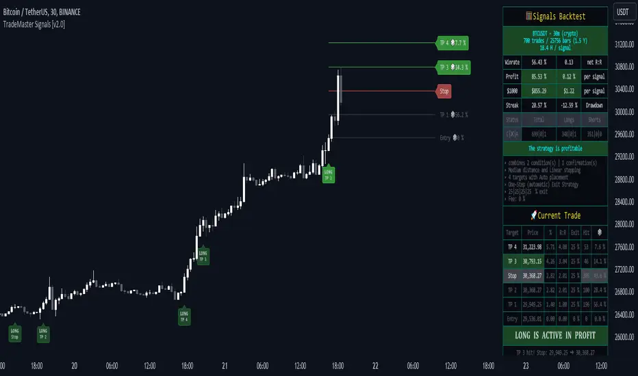
GKD-BT Multi-Ticker CC Backtest [Loxx]The Giga Kaleidoscope GKD-BT Multi-Ticker CC Backtest is a backtest module included in Loxx's "Giga Kaleidoscope Modularized Trading System."
█ Giga Kaleidoscope GKD-BT Multi-Ticker CC Backtest
This backtest allows you to test GKD-C Confirmation 1 and GKD-C Confirmation 2 indicators together without the hassle of adding additional confluence indicators. The backtest includes 1 take profit and 1 SL and various types of volatility. The backtest results on the chart are using 10% equity of 1 million total equity and $5 commission per trade.
To use this indicator:
1. Import the value "Input into NEW GKD-BT Backtest" from the GKD-C Confirmation 1 indicator into the GKD-BT Multi-Ticker CC Backtest.
2. Import the value "Input into NEW GKD-BT Backtest" from the GKD-C Confirmation 2 indicator into the GKD-BT Multi-Ticker CC Backtest.
This backtest includes the following metrics:
1. Net profit: Overall profit or loss achieved.
2. Total Closed Trades: Total number of closed trades, both winning and losing.
3. Total Percent Wins: Total wins, whether long or short, for the selected time interval regardless of commissions and other profit-modifying addons.
4. Percent Profitable: Total wins, whether long or short, that are also profitable, taking commissions into account.
5. Profit Factor: The ratio of gross profits to gross losses, indicating how much money the strategy made for every unit of money it lost.
6. Average Profit per Trade: The average gain or loss per trade, calculated by dividing the net profit by the total number of closed trades.
7. Average Number of Bars in Trade: The average number of bars that elapsed during trades for all closed trades.
Summary of notable settings:
Input Tickers separated by commas: Allows the user to input tickers separated by commas, specifying the symbols or tickers of financial instruments used in the backtest. The tickers should follow the format "EXCHANGE:TICKER" (e.g., "NASDAQ:AAPL, NYSE:MSFT").
Import GKD-B Baseline: Imports the "GKD-B Baseline" indicator.
Import GKD-V Volatility/Volume: Imports the "GKD-V Volatility/Volume" indicator.
Import GKD-C Confirmation: Imports the "GKD-C Confirmation" indicator.
Import GKD-C Continuation: Imports the "GKD-C Continuation" indicator.
Initial Capital: Represents the starting account balance for the backtest, denominated in the base currency of the trading account.
Order Size: Determines the quantity of contracts traded in each trade.
Order Type: Specifies the type of order used in the backtest, either "Contracts" or "% Equity."
Commission: Represents the commission per order or transaction cost incurred in each trade.
█ Giga Kaleidoscope Modularized Trading System
Core components of an NNFX algorithmic trading strategy
The NNFX algorithm is built on the principles of trend, momentum, and volatility. There are six core components in the NNFX trading algorithm:
1. Volatility - price volatility; e.g., Average True Range, True Range Double, Close-to-Close, etc.
2. Baseline - a moving average to identify price trend
3. Confirmation 1 - a technical indicator used to identify trends
4. Confirmation 2 - a technical indicator used to identify trends
5. Continuation - a technical indicator used to identify trends
6. Volatility/Volume - a technical indicator used to identify volatility/volume breakouts/breakdown
7. Exit - a technical indicator used to determine when a trend is exhausted
8. Metamorphosis - a technical indicator that produces a compound signal from the combination of other GKD indicators*
*(not part of the NNFX algorithm)
What is Volatility in the NNFX trading system?
In the NNFX (No Nonsense Forex) trading system, ATR (Average True Range) is typically used to measure the volatility of an asset. It is used as a part of the system to help determine the appropriate stop loss and take profit levels for a trade. ATR is calculated by taking the average of the true range values over a specified period.
True range is calculated as the maximum of the following values:
-Current high minus the current low
-Absolute value of the current high minus the previous close
-Absolute value of the current low minus the previous close
ATR is a dynamic indicator that changes with changes in volatility. As volatility increases, the value of ATR increases, and as volatility decreases, the value of ATR decreases. By using ATR in NNFX system, traders can adjust their stop loss and take profit levels according to the volatility of the asset being traded. This helps to ensure that the trade is given enough room to move, while also minimizing potential losses.
Other types of volatility include True Range Double (TRD), Close-to-Close, and Garman-Klass
What is a Baseline indicator?
The baseline is essentially a moving average, and is used to determine the overall direction of the market.
The baseline in the NNFX system is used to filter out trades that are not in line with the long-term trend of the market. The baseline is plotted on the chart along with other indicators, such as the Moving Average (MA), the Relative Strength Index (RSI), and the Average True Range (ATR).
Trades are only taken when the price is in the same direction as the baseline. For example, if the baseline is sloping upwards, only long trades are taken, and if the baseline is sloping downwards, only short trades are taken. This approach helps to ensure that trades are in line with the overall trend of the market, and reduces the risk of entering trades that are likely to fail.
By using a baseline in the NNFX system, traders can have a clear reference point for determining the overall trend of the market, and can make more informed trading decisions. The baseline helps to filter out noise and false signals, and ensures that trades are taken in the direction of the long-term trend.
What is a Confirmation indicator?
Confirmation indicators are technical indicators that are used to confirm the signals generated by primary indicators. Primary indicators are the core indicators used in the NNFX system, such as the Average True Range (ATR), the Moving Average (MA), and the Relative Strength Index (RSI).
The purpose of the confirmation indicators is to reduce false signals and improve the accuracy of the trading system. They are designed to confirm the signals generated by the primary indicators by providing additional information about the strength and direction of the trend.
Some examples of confirmation indicators that may be used in the NNFX system include the Bollinger Bands, the MACD (Moving Average Convergence Divergence), and the MACD Oscillator. These indicators can provide information about the volatility, momentum, and trend strength of the market, and can be used to confirm the signals generated by the primary indicators.
In the NNFX system, confirmation indicators are used in combination with primary indicators and other filters to create a trading system that is robust and reliable. By using multiple indicators to confirm trading signals, the system aims to reduce the risk of false signals and improve the overall profitability of the trades.
What is a Continuation indicator?
In the NNFX (No Nonsense Forex) trading system, a continuation indicator is a technical indicator that is used to confirm a current trend and predict that the trend is likely to continue in the same direction. A continuation indicator is typically used in conjunction with other indicators in the system, such as a baseline indicator, to provide a comprehensive trading strategy.
What is a Volatility/Volume indicator?
Volume indicators, such as the On Balance Volume (OBV), the Chaikin Money Flow (CMF), or the Volume Price Trend (VPT), are used to measure the amount of buying and selling activity in a market. They are based on the trading volume of the market, and can provide information about the strength of the trend. In the NNFX system, volume indicators are used to confirm trading signals generated by the Moving Average and the Relative Strength Index. Volatility indicators include Average Direction Index, Waddah Attar, and Volatility Ratio. In the NNFX trading system, volatility is a proxy for volume and vice versa.
By using volume indicators as confirmation tools, the NNFX trading system aims to reduce the risk of false signals and improve the overall profitability of trades. These indicators can provide additional information about the market that is not captured by the primary indicators, and can help traders to make more informed trading decisions. In addition, volume indicators can be used to identify potential changes in market trends and to confirm the strength of price movements.
What is an Exit indicator?
The exit indicator is used in conjunction with other indicators in the system, such as the Moving Average (MA), the Relative Strength Index (RSI), and the Average True Range (ATR), to provide a comprehensive trading strategy.
The exit indicator in the NNFX system can be any technical indicator that is deemed effective at identifying optimal exit points. Examples of exit indicators that are commonly used include the Parabolic SAR, the Average Directional Index (ADX), and the Chandelier Exit.
The purpose of the exit indicator is to identify when a trend is likely to reverse or when the market conditions have changed, signaling the need to exit a trade. By using an exit indicator, traders can manage their risk and prevent significant losses.
In the NNFX system, the exit indicator is used in conjunction with a stop loss and a take profit order to maximize profits and minimize losses. The stop loss order is used to limit the amount of loss that can be incurred if the trade goes against the trader, while the take profit order is used to lock in profits when the trade is moving in the trader's favor.
Overall, the use of an exit indicator in the NNFX trading system is an important component of a comprehensive trading strategy. It allows traders to manage their risk effectively and improve the profitability of their trades by exiting at the right time.
What is an Metamorphosis indicator?
The concept of a metamorphosis indicator involves the integration of two or more GKD indicators to generate a compound signal. This is achieved by evaluating the accuracy of each indicator and selecting the signal from the indicator with the highest accuracy. As an illustration, let's consider a scenario where we calculate the accuracy of 10 indicators and choose the signal from the indicator that demonstrates the highest accuracy.
The resulting output from the metamorphosis indicator can then be utilized in a GKD-BT backtest by occupying a slot that aligns with the purpose of the metamorphosis indicator. The slot can be a GKD-B, GKD-C, or GKD-E slot, depending on the specific requirements and objectives of the indicator. This allows for seamless integration and utilization of the compound signal within the GKD-BT framework.
How does Loxx's GKD (Giga Kaleidoscope Modularized Trading System) implement the NNFX algorithm outlined above?
Loxx's GKD v2.0 system has five types of modules (indicators/strategies). These modules are:
1. GKD-BT - Backtesting module (Volatility, Number 1 in the NNFX algorithm)
2. GKD-B - Baseline module (Baseline and Volatility/Volume, Numbers 1 and 2 in the NNFX algorithm)
3. GKD-C - Confirmation 1/2 and Continuation module (Confirmation 1/2 and Continuation, Numbers 3, 4, and 5 in the NNFX algorithm)
4. GKD-V - Volatility/Volume module (Confirmation 1/2, Number 6 in the NNFX algorithm)
5. GKD-E - Exit module (Exit, Number 7 in the NNFX algorithm)
6. GKD-M - Metamorphosis module (Metamorphosis, Number 8 in the NNFX algorithm, but not part of the NNFX algorithm)
(additional module types will added in future releases)
Each module interacts with every module by passing data to A backtest module wherein the various components of the GKD system are combined to create a trading signal.
That is, the Baseline indicator passes its data to Volatility/Volume. The Volatility/Volume indicator passes its values to the Confirmation 1 indicator. The Confirmation 1 indicator passes its values to the Confirmation 2 indicator. The Confirmation 2 indicator passes its values to the Continuation indicator. The Continuation indicator passes its values to the Exit indicator, and finally, the Exit indicator passes its values to the Backtest strategy.
This chaining of indicators requires that each module conform to Loxx's GKD protocol, therefore allowing for the testing of every possible combination of technical indicators that make up the six components of the NNFX algorithm.
What does the application of the GKD trading system look like?
Example trading system:
Backtest: Multi-Ticker CC Backtest as shown on the chart above
Baseline: Hull Moving Average
Volatility/Volume: Hurst Exponent
Confirmation 1: Fisher Transform as shown on the chart above
Confirmation 2: uf2018 as shown on the chart above
Continuation: Coppock Curve
Exit: Rex Oscillator
Metamorphosis: Baseline Optimizer
Each GKD indicator is denoted with a module identifier of either: GKD-BT, GKD-B, GKD-C, GKD-V, GKD-M, or GKD-E. This allows traders to understand to which module each indicator belongs and where each indicator fits into the GKD system.
█ Giga Kaleidoscope Modularized Trading System Signals
Standard Entry
1. GKD-C Confirmation gives signal
2. Baseline agrees
3. Price inside Goldie Locks Zone Minimum
4. Price inside Goldie Locks Zone Maximum
5. Confirmation 2 agrees
6. Volatility/Volume agrees
1-Candle Standard Entry
1a. GKD-C Confirmation gives signal
2a. Baseline agrees
3a. Price inside Goldie Locks Zone Minimum
4a. Price inside Goldie Locks Zone Maximum
Next Candle
1b. Price retraced
2b. Baseline agrees
3b. Confirmation 1 agrees
4b. Confirmation 2 agrees
5b. Volatility/Volume agrees
Baseline Entry
1. GKD-B Baseline gives signal
2. Confirmation 1 agrees
3. Price inside Goldie Locks Zone Minimum
4. Price inside Goldie Locks Zone Maximum
5. Confirmation 2 agrees
6. Volatility/Volume agrees
7. Confirmation 1 signal was less than 'Maximum Allowable PSBC Bars Back' prior
1-Candle Baseline Entry
1a. GKD-B Baseline gives signal
2a. Confirmation 1 agrees
3a. Price inside Goldie Locks Zone Minimum
4a. Price inside Goldie Locks Zone Maximum
5a. Confirmation 1 signal was less than 'Maximum Allowable PSBC Bars Back' prior
Next Candle
1b. Price retraced
2b. Baseline agrees
3b. Confirmation 1 agrees
4b. Confirmation 2 agrees
5b. Volatility/Volume agrees
Volatility/Volume Entry
1. GKD-V Volatility/Volume gives signal
2. Confirmation 1 agrees
3. Price inside Goldie Locks Zone Minimum
4. Price inside Goldie Locks Zone Maximum
5. Confirmation 2 agrees
6. Baseline agrees
7. Confirmation 1 signal was less than 7 candles prior
1-Candle Volatility/Volume Entry
1a. GKD-V Volatility/Volume gives signal
2a. Confirmation 1 agrees
3a. Price inside Goldie Locks Zone Minimum
4a. Price inside Goldie Locks Zone Maximum
5a. Confirmation 1 signal was less than 'Maximum Allowable PSVVC Bars Back' prior
Next Candle
1b. Price retraced
2b. Volatility/Volume agrees
3b. Confirmation 1 agrees
4b. Confirmation 2 agrees
5b. Baseline agrees
Confirmation 2 Entry
1. GKD-C Confirmation 2 gives signal
2. Confirmation 1 agrees
3. Price inside Goldie Locks Zone Minimum
4. Price inside Goldie Locks Zone Maximum
5. Volatility/Volume agrees
6. Baseline agrees
7. Confirmation 1 signal was less than 7 candles prior
1-Candle Confirmation 2 Entry
1a. GKD-C Confirmation 2 gives signal
2a. Confirmation 1 agrees
3a. Price inside Goldie Locks Zone Minimum
4a. Price inside Goldie Locks Zone Maximum
5a. Confirmation 1 signal was less than 'Maximum Allowable PSC2C Bars Back' prior
Next Candle
1b. Price retraced
2b. Confirmation 2 agrees
3b. Confirmation 1 agrees
4b. Volatility/Volume agrees
5b. Baseline agrees
PullBack Entry
1a. GKD-B Baseline gives signal
2a. Confirmation 1 agrees
3a. Price is beyond 1.0x Volatility of Baseline
Next Candle
1b. Price inside Goldie Locks Zone Minimum
2b. Price inside Goldie Locks Zone Maximum
3b. Confirmation 1 agrees
4b. Confirmation 2 agrees
5b. Volatility/Volume agrees
Continuation Entry
1. Standard Entry, 1-Candle Standard Entry, Baseline Entry, 1-Candle Baseline Entry, Volatility/Volume Entry, 1-Candle Volatility/Volume Entry, Confirmation 2 Entry, 1-Candle Confirmation 2 Entry, or Pullback entry triggered previously
2. Baseline hasn't crossed since entry signal trigger
4. Confirmation 1 agrees
5. Baseline agrees
6. Confirmation 2 agrees
█ Connecting to Backtests
All GKD indicators are chained indicators meaning you export the value of the indicators to specialized backtest to creat your GKD trading system. Each indicator contains a proprietary signal generation algo that will only work with GKD backtests. You can find these backtests using the links below.
GKD-BT Giga Confirmation Stack Backtest
GKD-BT Giga Stacks Backtest
GKD-BT Full Giga Kaleidoscope Backtest
GKD-BT Solo Confirmation Super Complex Backtest
GKD-BT Solo Confirmation Complex Backtest
GKD-BT Solo Confirmation Simple Backtest
GKD-M Baseline Optimizer
GKD-M Accuracy Alchemist
GKD-BT Multi-Ticker SCC Backtest
GKD-BT Multi-Ticker SCS Backtest
GKD-BT Multi-Ticker SCS Backtest
GKD-BT Multi-Ticker Full GKD Backtest
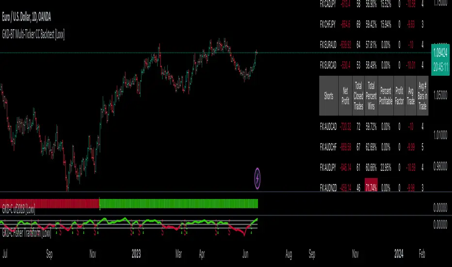
GKD-BT Optimizer SCC Backtest [Loxx]The Giga Kaleidoscope GKD-BT Optimizer SCC Backtest is a backtesting module included in Loxx's "Giga Kaleidoscope Modularized Trading System."
█ Giga Kaleidoscope GKD-BT Optimizer SCC Backtest
The Optimizer SCC Backtest is a Solo Confirmation Complex backtest that allows traders to test single GKD-C Confirmation indicator with GKD-B Baseline and GKD-V Volatility/Volume filtering across 10 varying inputs. The purpose of this backtest is to enable traders to optimize a GKD-C indicator given varying inputs.
The backtest module supports testing with 1 take profit and 1 stop loss. It also offers the option to limit testing to a specific date range, allowing simulated forward testing using historical data. This backtest module only includes standard long and short signals. Additionally, users can choose to display or hide a trading panel that provides relevant information about the backtest, statistics, and the current trade. Traders can also select a highlighting treshold for Total Percent Wins and Percent Profitable, and Profit Factor.
To use this indicator:
1. Import the value "Input into NEW GKD-BT Backtest" from the GKD-B Baseline indicator into the GKD-BT Optimizer SCC Backtest.
2. Import the value "Input into NEW GKD-BT Backtest" from the GKD-V Volatility/Volume indicator into the GKD-BT Optimizer SCC Backtest.
3. Select the "Optimizer" option in the GKD-C Confirmation indicator
4. Import a GKD-C indicator "Input into NEW GKD-BT Optimizer Backtest Signals" into the GKD-C Indicator Signals dropdown
5. Import a GKD-C indicator "Input into NEW GKD-BT Optimizer Backtest Start" into the GKD-C Indicator Start dropdown
6. Import a GKD-C indicator "Input into NEW GKD-BT Optimizer Backtest Skip" into the GKD-C Indicator Skip dropdown
This backtest includes the following metrics:
1. Net profit: Overall profit or loss achieved.
2. Total Closed Trades: Total number of closed trades, both winning and losing.
3. Total Percent Wins: Total wins, whether long or short, for the selected time interval regardless of commissions and other profit-modifying addons.
4. Percent Profitable: Total wins, whether long or short, that are also profitable, taking commissions into account.
5. Profit Factor: The ratio of gross profits to gross losses, indicating how much money the strategy made for every unit of money it lost.
6. Average Profit per Trade: The average gain or loss per trade, calculated by dividing the net profit by the total number of closed trades.
7. Average Number of Bars in Trade: The average number of bars that elapsed during trades for all closed trades.
Summary of notable settings:
Input Tickers separated by commas: Allows the user to input tickers separated by commas, specifying the symbols or tickers of financial instruments used in the backtest. The tickers should follow the format "EXCHANGE:TICKER" (e.g., "NASDAQ:AAPL, NYSE:MSFT").
Import GKD-B Baseline: Imports the "GKD-B Baseline" indicator.
Import GKD-V Volatility/Volume: Imports the "GKD-V Volatility/Volume" indicator.
Import GKD-C Confirmation: Imports the "GKD-C Confirmation" indicator.
Import GKD-C Continuation: Imports the "GKD-C Continuation" indicator.
Initial Capital: Represents the starting account balance for the backtest, denominated in the base currency of the trading account.
Order Size: Determines the quantity of contracts traded in each trade.
Order Type: Specifies the type of order used in the backtest, either "Contracts" or "% Equity."
Commission: Represents the commission per order or transaction cost incurred in each trade.
**the backtest data rendered to the chart above uses $5 commission per trade and 10% equity per trade with $1 million initial capital. Each backtest result for each ticker assumes these same inputs. The results are NOT cumulative, they are separate and isolate per ticker and trading side, long or short**
█ Volatility Types included
The GKD system utilizes volatility-based take profits and stop losses. Each take profit and stop loss is calculated as a multiple of volatility. You can change the values of the multipliers in the settings as well.
This module includes 17 types of volatility:
Close-to-Close
Parkinson
Garman-Klass
Rogers-Satchell
Yang-Zhang
Garman-Klass-Yang-Zhang
Exponential Weighted Moving Average
Standard Deviation of Log Returns
Pseudo GARCH(2,2)
Average True Range
True Range Double
Standard Deviation
Adaptive Deviation
Median Absolute Deviation
Efficiency-Ratio Adaptive ATR
Mean Absolute Deviation
Static Percent
Various volatility estimators and indicators that investors and traders can use to measure the dispersion or volatility of a financial instrument's price. Each estimator has its strengths and weaknesses, and the choice of estimator should depend on the specific needs and circumstances of the user.
Close-to-Close
Close-to-Close volatility is a classic and widely used volatility measure, sometimes referred to as historical volatility.
Volatility is an indicator of the speed of a stock price change. A stock with high volatility is one where the price changes rapidly and with a larger amplitude. The more volatile a stock is, the riskier it is.
Close-to-close historical volatility is calculated using only a stock's closing prices. It is the simplest volatility estimator. However, in many cases, it is not precise enough. Stock prices could jump significantly during a trading session and return to the opening value at the end. That means that a considerable amount of price information is not taken into account by close-to-close volatility.
Despite its drawbacks, Close-to-Close volatility is still useful in cases where the instrument doesn't have intraday prices. For example, mutual funds calculate their net asset values daily or weekly, and thus their prices are not suitable for more sophisticated volatility estimators.
Parkinson
Parkinson volatility is a volatility measure that uses the stock’s high and low price of the day.
The main difference between regular volatility and Parkinson volatility is that the latter uses high and low prices for a day, rather than only the closing price. This is useful as close-to-close prices could show little difference while large price movements could have occurred during the day. Thus, Parkinson's volatility is considered more precise and requires less data for calculation than close-to-close volatility.
One drawback of this estimator is that it doesn't take into account price movements after the market closes. Hence, it systematically undervalues volatility. This drawback is addressed in the Garman-Klass volatility estimator.
Garman-Klass
Garman-Klass is a volatility estimator that incorporates open, low, high, and close prices of a security.
Garman-Klass volatility extends Parkinson's volatility by taking into account the opening and closing prices. As markets are most active during the opening and closing of a trading session, it makes volatility estimation more accurate.
Garman and Klass also assumed that the process of price change follows a continuous diffusion process (Geometric Brownian motion). However, this assumption has several drawbacks. The method is not robust for opening jumps in price and trend movements.
Despite its drawbacks, the Garman-Klass estimator is still more effective than the basic formula since it takes into account not only the price at the beginning and end of the time interval but also intraday price extremes.
Researchers Rogers and Satchell have proposed a more efficient method for assessing historical volatility that takes into account price trends. See Rogers-Satchell Volatility for more detail.
Rogers-Satchell
Rogers-Satchell is an estimator for measuring the volatility of securities with an average return not equal to zero.
Unlike Parkinson and Garman-Klass estimators, Rogers-Satchell incorporates a drift term (mean return not equal to zero). As a result, it provides better volatility estimation when the underlying is trending.
The main disadvantage of this method is that it does not take into account price movements between trading sessions. This leads to an underestimation of volatility since price jumps periodically occur in the market precisely at the moments between sessions.
A more comprehensive estimator that also considers the gaps between sessions was developed based on the Rogers-Satchel formula in the 2000s by Yang-Zhang. See Yang Zhang Volatility for more detail.
Yang-Zhang
Yang Zhang is a historical volatility estimator that handles both opening jumps and the drift and has a minimum estimation error.
Yang-Zhang volatility can be thought of as a combination of the overnight (close-to-open volatility) and a weighted average of the Rogers-Satchell volatility and the day’s open-to-close volatility. It is considered to be 14 times more efficient than the close-to-close estimator.
Garman-Klass-Yang-Zhang
Garman-Klass-Yang-Zhang (GKYZ) volatility estimator incorporates the returns of open, high, low, and closing prices in its calculation.
GKYZ volatility estimator takes into account overnight jumps but not the trend, i.e., it assumes that the underlying asset follows a Geometric Brownian Motion (GBM) process with zero drift. Therefore, the GKYZ volatility estimator tends to overestimate the volatility when the drift is different from zero. However, for a GBM process, this estimator is eight times more efficient than the close-to-close volatility estimator.
Exponential Weighted Moving Average
The Exponentially Weighted Moving Average (EWMA) is a quantitative or statistical measure used to model or describe a time series. The EWMA is widely used in finance, with the main applications being technical analysis and volatility modeling.
The moving average is designed such that older observations are given lower weights. The weights decrease exponentially as the data point gets older – hence the name exponentially weighted.
The only decision a user of the EWMA must make is the parameter lambda. The parameter decides how important the current observation is in the calculation of the EWMA. The higher the value of lambda, the more closely the EWMA tracks the original time series.
Standard Deviation of Log Returns
This is the simplest calculation of volatility. It's the standard deviation of ln(close/close(1)).
Pseudo GARCH(2,2)
This is calculated using a short- and long-run mean of variance multiplied by ?.
?avg(var;M) + (1 ? ?) avg(var;N) = 2?var/(M+1-(M-1)L) + 2(1-?)var/(M+1-(M-1)L)
Solving for ? can be done by minimizing the mean squared error of estimation; that is, regressing L^-1var - avg(var; N) against avg(var; M) - avg(var; N) and using the resulting beta estimate as ?.
Average True Range
The average true range (ATR) is a technical analysis indicator, introduced by market technician J. Welles Wilder Jr. in his book New Concepts in Technical Trading Systems, that measures market volatility by decomposing the entire range of an asset price for that period.
The true range indicator is taken as the greatest of the following: current high less the current low; the absolute value of the current high less the previous close; and the absolute value of the current low less the previous close. The ATR is then a moving average, generally using 14 days, of the true ranges.
True Range Double
A special case of ATR that attempts to correct for volatility skew.
Standard Deviation
Standard deviation is a statistic that measures the dispersion of a dataset relative to its mean and is calculated as the square root of the variance. The standard deviation is calculated as the square root of variance by determining each data point's deviation relative to the mean. If the data points are further from the mean, there is a higher deviation within the data set; thus, the more spread out the data, the higher the standard deviation.
Adaptive Deviation
By definition, the Standard Deviation (STD, also represented by the Greek letter sigma ? or the Latin letter s) is a measure that is used to quantify the amount of variation or dispersion of a set of data values. In technical analysis, we usually use it to measure the level of current volatility.
Standard Deviation is based on Simple Moving Average calculation for mean value. This version of standard deviation uses the properties of EMA to calculate what can be called a new type of deviation, and since it is based on EMA, we can call it EMA deviation. Additionally, Perry Kaufman's efficiency ratio is used to make it adaptive (since all EMA type calculations are nearly perfect for adapting).
The difference when compared to the standard is significant--not just because of EMA usage, but the efficiency ratio makes it a "bit more logical" in very volatile market conditions.
Median Absolute Deviation
The median absolute deviation is a measure of statistical dispersion. Moreover, the MAD is a robust statistic, being more resilient to outliers in a data set than the standard deviation. In the standard deviation, the distances from the mean are squared, so large deviations are weighted more heavily, and thus outliers can heavily influence it. In the MAD, the deviations of a small number of outliers are irrelevant.
Because the MAD is a more robust estimator of scale than the sample variance or standard deviation, it works better with distributions without a mean or variance, such as the Cauchy distribution.
For this indicator, a manual recreation of the quantile function in Pine Script is used. This is so users have a full inside view into how this is calculated.
Efficiency-Ratio Adaptive ATR
Average True Range (ATR) is a widely used indicator for many occasions in technical analysis. It is calculated as the RMA of the true range. This version adds a "twist": it uses Perry Kaufman's Efficiency Ratio to calculate adaptive true range.
Mean Absolute Deviation
The mean absolute deviation (MAD) is a measure of variability that indicates the average distance between observations and their mean. MAD uses the original units of the data, which simplifies interpretation. Larger values signify that the data points spread out further from the average. Conversely, lower values correspond to data points bunching closer to it. The mean absolute deviation is also known as the mean deviation and average absolute deviation.
This definition of the mean absolute deviation sounds similar to the standard deviation (SD). While both measure variability, they have different calculations. In recent years, some proponents of MAD have suggested that it replace the SD as the primary measure because it is a simpler concept that better fits real life.
█ Giga Kaleidoscope Modularized Trading System
Core components of an NNFX algorithmic trading strategy
The NNFX algorithm is built on the principles of trend, momentum, and volatility. There are six core components in the NNFX trading algorithm:
1. Volatility - price volatility; e.g., Average True Range, True Range Double, Close-to-Close, etc.
2. Baseline - a moving average to identify price trend
3. Confirmation 1 - a technical indicator used to identify trends
4. Confirmation 2 - a technical indicator used to identify trends
5. Continuation - a technical indicator used to identify trends
6. Volatility/Volume - a technical indicator used to identify volatility/volume breakouts/breakdown
7. Exit - a technical indicator used to determine when a trend is exhausted
8. Metamorphosis - a technical indicator that produces a compound signal from the combination of other GKD indicators*
*(not part of the NNFX algorithm)
What is Volatility in the NNFX trading system?
In the NNFX (No Nonsense Forex) trading system, ATR (Average True Range) is typically used to measure the volatility of an asset. It is used as a part of the system to help determine the appropriate stop loss and take profit levels for a trade. ATR is calculated by taking the average of the true range values over a specified period.
True range is calculated as the maximum of the following values:
-Current high minus the current low
-Absolute value of the current high minus the previous close
-Absolute value of the current low minus the previous close
ATR is a dynamic indicator that changes with changes in volatility. As volatility increases, the value of ATR increases, and as volatility decreases, the value of ATR decreases. By using ATR in NNFX system, traders can adjust their stop loss and take profit levels according to the volatility of the asset being traded. This helps to ensure that the trade is given enough room to move, while also minimizing potential losses.
Other types of volatility include True Range Double (TRD), Close-to-Close, and Garman-Klass
What is a Baseline indicator?
The baseline is essentially a moving average, and is used to determine the overall direction of the market.
The baseline in the NNFX system is used to filter out trades that are not in line with the long-term trend of the market. The baseline is plotted on the chart along with other indicators, such as the Moving Average (MA), the Relative Strength Index (RSI), and the Average True Range (ATR).
Trades are only taken when the price is in the same direction as the baseline. For example, if the baseline is sloping upwards, only long trades are taken, and if the baseline is sloping downwards, only short trades are taken. This approach helps to ensure that trades are in line with the overall trend of the market, and reduces the risk of entering trades that are likely to fail.
By using a baseline in the NNFX system, traders can have a clear reference point for determining the overall trend of the market, and can make more informed trading decisions. The baseline helps to filter out noise and false signals, and ensures that trades are taken in the direction of the long-term trend.
What is a Confirmation indicator?
Confirmation indicators are technical indicators that are used to confirm the signals generated by primary indicators. Primary indicators are the core indicators used in the NNFX system, such as the Average True Range (ATR), the Moving Average (MA), and the Relative Strength Index (RSI).
The purpose of the confirmation indicators is to reduce false signals and improve the accuracy of the trading system. They are designed to confirm the signals generated by the primary indicators by providing additional information about the strength and direction of the trend.
Some examples of confirmation indicators that may be used in the NNFX system include the Bollinger Bands, the MACD (Moving Average Convergence Divergence), and the MACD Oscillator. These indicators can provide information about the volatility, momentum, and trend strength of the market, and can be used to confirm the signals generated by the primary indicators.
In the NNFX system, confirmation indicators are used in combination with primary indicators and other filters to create a trading system that is robust and reliable. By using multiple indicators to confirm trading signals, the system aims to reduce the risk of false signals and improve the overall profitability of the trades.
What is a Continuation indicator?
In the NNFX (No Nonsense Forex) trading system, a continuation indicator is a technical indicator that is used to confirm a current trend and predict that the trend is likely to continue in the same direction. A continuation indicator is typically used in conjunction with other indicators in the system, such as a baseline indicator, to provide a comprehensive trading strategy.
What is a Volatility/Volume indicator?
Volume indicators, such as the On Balance Volume (OBV), the Chaikin Money Flow (CMF), or the Volume Price Trend (VPT), are used to measure the amount of buying and selling activity in a market. They are based on the trading volume of the market, and can provide information about the strength of the trend. In the NNFX system, volume indicators are used to confirm trading signals generated by the Moving Average and the Relative Strength Index. Volatility indicators include Average Direction Index, Waddah Attar, and Volatility Ratio. In the NNFX trading system, volatility is a proxy for volume and vice versa.
By using volume indicators as confirmation tools, the NNFX trading system aims to reduce the risk of false signals and improve the overall profitability of trades. These indicators can provide additional information about the market that is not captured by the primary indicators, and can help traders to make more informed trading decisions. In addition, volume indicators can be used to identify potential changes in market trends and to confirm the strength of price movements.
What is an Exit indicator?
The exit indicator is used in conjunction with other indicators in the system, such as the Moving Average (MA), the Relative Strength Index (RSI), and the Average True Range (ATR), to provide a comprehensive trading strategy.
The exit indicator in the NNFX system can be any technical indicator that is deemed effective at identifying optimal exit points. Examples of exit indicators that are commonly used include the Parabolic SAR, the Average Directional Index (ADX), and the Chandelier Exit.
The purpose of the exit indicator is to identify when a trend is likely to reverse or when the market conditions have changed, signaling the need to exit a trade. By using an exit indicator, traders can manage their risk and prevent significant losses.
In the NNFX system, the exit indicator is used in conjunction with a stop loss and a take profit order to maximize profits and minimize losses. The stop loss order is used to limit the amount of loss that can be incurred if the trade goes against the trader, while the take profit order is used to lock in profits when the trade is moving in the trader's favor.
Overall, the use of an exit indicator in the NNFX trading system is an important component of a comprehensive trading strategy. It allows traders to manage their risk effectively and improve the profitability of their trades by exiting at the right time.
What is an Metamorphosis indicator?
The concept of a metamorphosis indicator involves the integration of two or more GKD indicators to generate a compound signal. This is achieved by evaluating the accuracy of each indicator and selecting the signal from the indicator with the highest accuracy. As an illustration, let's consider a scenario where we calculate the accuracy of 10 indicators and choose the signal from the indicator that demonstrates the highest accuracy.
The resulting output from the metamorphosis indicator can then be utilized in a GKD-BT backtest by occupying a slot that aligns with the purpose of the metamorphosis indicator. The slot can be a GKD-B, GKD-C, or GKD-E slot, depending on the specific requirements and objectives of the indicator. This allows for seamless integration and utilization of the compound signal within the GKD-BT framework.
How does Loxx's GKD (Giga Kaleidoscope Modularized Trading System) implement the NNFX algorithm outlined above?
Loxx's GKD v2.0 system has five types of modules (indicators/strategies). These modules are:
1. GKD-BT - Backtesting module (Volatility, Number 1 in the NNFX algorithm)
2. GKD-B - Baseline module (Baseline and Volatility/Volume, Numbers 1 and 2 in the NNFX algorithm)
3. GKD-C - Confirmation 1/2 and Continuation module (Confirmation 1/2 and Continuation, Numbers 3, 4, and 5 in the NNFX algorithm)
4. GKD-V - Volatility/Volume module (Confirmation 1/2, Number 6 in the NNFX algorithm)
5. GKD-E - Exit module (Exit, Number 7 in the NNFX algorithm)
6. GKD-M - Metamorphosis module (Metamorphosis, Number 8 in the NNFX algorithm, but not part of the NNFX algorithm)
(additional module types will added in future releases)
Each module interacts with every module by passing data to A backtest module wherein the various components of the GKD system are combined to create a trading signal.
That is, the Baseline indicator passes its data to Volatility/Volume. The Volatility/Volume indicator passes its values to the Confirmation 1 indicator. The Confirmation 1 indicator passes its values to the Confirmation 2 indicator. The Confirmation 2 indicator passes its values to the Continuation indicator. The Continuation indicator passes its values to the Exit indicator, and finally, the Exit indicator passes its values to the Backtest strategy.
This chaining of indicators requires that each module conform to Loxx's GKD protocol, therefore allowing for the testing of every possible combination of technical indicators that make up the six components of the NNFX algorithm.
What does the application of the GKD trading system look like?
Example trading system:
Backtest: Optimizer Full GKD Backtest as shown on the chart above
Baseline: Hull Moving Average
Volatility/Volume: Hurst Exponent
Confirmation 1: Fisher Transofrm as shown on the chart above
Confirmation 2: uf2018
Continuation: Coppock Curve
Exit: Rex Oscillator
Metamorphosis: Baseline Optimizer
Each GKD indicator is denoted with a module identifier of either: GKD-BT, GKD-B, GKD-C, GKD-V, GKD-M, or GKD-E. This allows traders to understand to which module each indicator belongs and where each indicator fits into the GKD system.
█ Giga Kaleidoscope Modularized Trading System Signals
Standard Entry
1. GKD-C Confirmation gives signal
2. Baseline agrees
3. Price inside Goldie Locks Zone Minimum
4. Price inside Goldie Locks Zone Maximum
5. Confirmation 2 agrees
6. Volatility/Volume agrees
1-Candle Standard Entry
1a. GKD-C Confirmation gives signal
2a. Baseline agrees
3a. Price inside Goldie Locks Zone Minimum
4a. Price inside Goldie Locks Zone Maximum
Next Candle
1b. Price retraced
2b. Baseline agrees
3b. Confirmation 1 agrees
4b. Confirmation 2 agrees
5b. Volatility/Volume agrees
Baseline Entry
1. GKD-B Baseline gives signal
2. Confirmation 1 agrees
3. Price inside Goldie Locks Zone Minimum
4. Price inside Goldie Locks Zone Maximum
5. Confirmation 2 agrees
6. Volatility/Volume agrees
7. Confirmation 1 signal was less than 'Maximum Allowable PSBC Bars Back' prior
1-Candle Baseline Entry
1a. GKD-B Baseline gives signal
2a. Confirmation 1 agrees
3a. Price inside Goldie Locks Zone Minimum
4a. Price inside Goldie Locks Zone Maximum
5a. Confirmation 1 signal was less than 'Maximum Allowable PSBC Bars Back' prior
Next Candle
1b. Price retraced
2b. Baseline agrees
3b. Confirmation 1 agrees
4b. Confirmation 2 agrees
5b. Volatility/Volume agrees
Volatility/Volume Entry
1. GKD-V Volatility/Volume gives signal
2. Confirmation 1 agrees
3. Price inside Goldie Locks Zone Minimum
4. Price inside Goldie Locks Zone Maximum
5. Confirmation 2 agrees
6. Baseline agrees
7. Confirmation 1 signal was less than 7 candles prior
1-Candle Volatility/Volume Entry
1a. GKD-V Volatility/Volume gives signal
2a. Confirmation 1 agrees
3a. Price inside Goldie Locks Zone Minimum
4a. Price inside Goldie Locks Zone Maximum
5a. Confirmation 1 signal was less than 'Maximum Allowable PSVVC Bars Back' prior
Next Candle
1b. Price retraced
2b. Volatility/Volume agrees
3b. Confirmation 1 agrees
4b. Confirmation 2 agrees
5b. Baseline agrees
Confirmation 2 Entry
1. GKD-C Confirmation 2 gives signal
2. Confirmation 1 agrees
3. Price inside Goldie Locks Zone Minimum
4. Price inside Goldie Locks Zone Maximum
5. Volatility/Volume agrees
6. Baseline agrees
7. Confirmation 1 signal was less than 7 candles prior
1-Candle Confirmation 2 Entry
1a. GKD-C Confirmation 2 gives signal
2a. Confirmation 1 agrees
3a. Price inside Goldie Locks Zone Minimum
4a. Price inside Goldie Locks Zone Maximum
5a. Confirmation 1 signal was less than 'Maximum Allowable PSC2C Bars Back' prior
Next Candle
1b. Price retraced
2b. Confirmation 2 agrees
3b. Confirmation 1 agrees
4b. Volatility/Volume agrees
5b. Baseline agrees
PullBack Entry
1a. GKD-B Baseline gives signal
2a. Confirmation 1 agrees
3a. Price is beyond 1.0x Volatility of Baseline
Next Candle
1b. Price inside Goldie Locks Zone Minimum
2b. Price inside Goldie Locks Zone Maximum
3b. Confirmation 1 agrees
4b. Confirmation 2 agrees
5b. Volatility/Volume agrees
Continuation Entry
1. Standard Entry, 1-Candle Standard Entry, Baseline Entry, 1-Candle Baseline Entry, Volatility/Volume Entry, 1-Candle Volatility/Volume Entry, Confirmation 2 Entry, 1-Candle Confirmation 2 Entry, or Pullback entry triggered previously
2. Baseline hasn't crossed since entry signal trigger
4. Confirmation 1 agrees
5. Baseline agrees
6. Confirmation 2 agrees
█ Connecting to Backtests
All GKD indicators are chained indicators meaning you export the value of the indicators to specialized backtest to creat your GKD trading system. Each indicator contains a proprietary signal generation algo that will only work with GKD backtests. You can find these backtests using the links below.
GKD-BT Giga Confirmation Stack Backtest
GKD-BT Giga Stacks Backtest
GKD-BT Full Giga Kaleidoscope Backtest
GKD-BT Solo Confirmation Super Complex Backtest
GKD-BT Solo Confirmation Complex Backtest
GKD-BT Solo Confirmation Simple Backtest
GKD-M Baseline Optimizer
GKD-M Accuracy Alchemist
GKD-BT Optimizer SCC Backtest
GKD-BT Optimizer SCC Backtest
GKD-BT Optimizer SCC Backtest
GKD-C GKD-BT Optimizer Full GKD Backtest
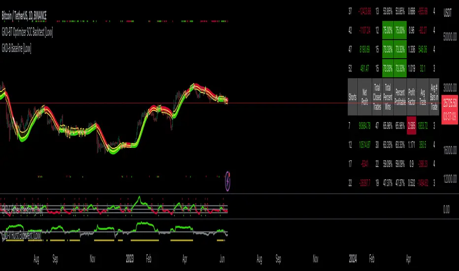
GKD-BT Optimizer SCS Backtest [Loxx]The Giga Kaleidoscope GKD-BT Optimizer SCS Backtest is a backtesting module included in Loxx's "Giga Kaleidoscope Modularized Trading System."
█ Giga Kaleidoscope GKD-BT Optimizer SCS Backtest
The Optimizer SCS Backtest is a Solo Confirmation Simple backtest that allows traders to test single GKD-C confirmation indicators across 10 varying inputs. The purpose of this backtest is to enable traders to optimize a GKD-C indicator given varying inputs.
The backtest module supports testing with 1 take profit and 1 stop loss. It also offers the option to limit testing to a specific date range, allowing simulated forward testing using historical data. This backtest module only includes standard long and short signals. Additionally, users can choose to display or hide a trading panel that provides relevant information about the backtest, statistics, and the current trade. Traders can also select a highlighting treshold for Total Percent Wins and Percent Profitable, and Profit Factor.
To use this indicator:
1. Import a GKD-C indicator "Input into NEW GKD-BT Optimizer Backtest Signals" into the GKD-C Indicator Signals dropdown
1. Import a GKD-C indicator "Input into NEW GKD-BT Optimizer Backtest Start" into the GKD-C Indicator Start dropdown
1. Import a GKD-C indicator "Input into NEW GKD-BT Optimizer Backtest Skip" into the GKD-C Indicator Skip dropdown
This backtest includes the following metrics:
1. Net profit: Overall profit or loss achieved.
2. Total Closed Trades: Total number of closed trades, both winning and losing.
3. Total Percent Wins: Total wins, whether long or short, for the selected time interval regardless of commissions and other profit-modifying addons.
4. Percent Profitable: Total wins, whether long or short, that are also profitable, taking commissions into account.
5. Profit Factor: The ratio of gross profits to gross losses, indicating how much money the strategy made for every unit of money it lost.
6. Average Profit per Trade: The average gain or loss per trade, calculated by dividing the net profit by the total number of closed trades.
7. Average Number of Bars in Trade: The average number of bars that elapsed during trades for all closed trades.
Summary of notable settings:
Input Tickers separated by commas: Allows the user to input tickers separated by commas, specifying the symbols or tickers of financial instruments used in the backtest. The tickers should follow the format "EXCHANGE:TICKER" (e.g., "NASDAQ:AAPL, NYSE:MSFT").
Import GKD-B Baseline: Imports the "GKD-B Multi-Ticker Baseline" indicator.
Import GKD-V Volatility/Volume: Imports the "GKD-V Volatility/Volume" indicator.
Import GKD-C Confirmation: Imports the "GKD-C Confirmation" indicator.
Import GKD-C Continuation: Imports the "GKD-C Continuation" indicator.
Initial Capital: Represents the starting account balance for the backtest, denominated in the base currency of the trading account.
Order Size: Determines the quantity of contracts traded in each trade.
Order Type: Specifies the type of order used in the backtest, either "Contracts" or "% Equity."
Commission: Represents the commission per order or transaction cost incurred in each trade.
**the backtest data rendered to the chart above uses $5 commission per trade and 10% equity per trade with $1 million initial capital. Each backtest result for each ticker assumes these same inputs. The results are NOT cumulative, they are separate and isolate per ticker and trading side, long or short**
█ Volatility Types included
The GKD system utilizes volatility-based take profits and stop losses. Each take profit and stop loss is calculated as a multiple of volatility. You can change the values of the multipliers in the settings as well.
This module includes 17 types of volatility:
Close-to-Close
Parkinson
Garman-Klass
Rogers-Satchell
Yang-Zhang
Garman-Klass-Yang-Zhang
Exponential Weighted Moving Average
Standard Deviation of Log Returns
Pseudo GARCH(2,2)
Average True Range
True Range Double
Standard Deviation
Adaptive Deviation
Median Absolute Deviation
Efficiency-Ratio Adaptive ATR
Mean Absolute Deviation
Static Percent
Various volatility estimators and indicators that investors and traders can use to measure the dispersion or volatility of a financial instrument's price. Each estimator has its strengths and weaknesses, and the choice of estimator should depend on the specific needs and circumstances of the user.
Close-to-Close
Close-to-Close volatility is a classic and widely used volatility measure, sometimes referred to as historical volatility.
Volatility is an indicator of the speed of a stock price change. A stock with high volatility is one where the price changes rapidly and with a larger amplitude. The more volatile a stock is, the riskier it is.
Close-to-close historical volatility is calculated using only a stock's closing prices. It is the simplest volatility estimator. However, in many cases, it is not precise enough. Stock prices could jump significantly during a trading session and return to the opening value at the end. That means that a considerable amount of price information is not taken into account by close-to-close volatility.
Despite its drawbacks, Close-to-Close volatility is still useful in cases where the instrument doesn't have intraday prices. For example, mutual funds calculate their net asset values daily or weekly, and thus their prices are not suitable for more sophisticated volatility estimators.
Parkinson
Parkinson volatility is a volatility measure that uses the stock’s high and low price of the day.
The main difference between regular volatility and Parkinson volatility is that the latter uses high and low prices for a day, rather than only the closing price. This is useful as close-to-close prices could show little difference while large price movements could have occurred during the day. Thus, Parkinson's volatility is considered more precise and requires less data for calculation than close-to-close volatility.
One drawback of this estimator is that it doesn't take into account price movements after the market closes. Hence, it systematically undervalues volatility. This drawback is addressed in the Garman-Klass volatility estimator.
Garman-Klass
Garman-Klass is a volatility estimator that incorporates open, low, high, and close prices of a security.
Garman-Klass volatility extends Parkinson's volatility by taking into account the opening and closing prices. As markets are most active during the opening and closing of a trading session, it makes volatility estimation more accurate.
Garman and Klass also assumed that the process of price change follows a continuous diffusion process (Geometric Brownian motion). However, this assumption has several drawbacks. The method is not robust for opening jumps in price and trend movements.
Despite its drawbacks, the Garman-Klass estimator is still more effective than the basic formula since it takes into account not only the price at the beginning and end of the time interval but also intraday price extremes.
Researchers Rogers and Satchell have proposed a more efficient method for assessing historical volatility that takes into account price trends. See Rogers-Satchell Volatility for more detail.
Rogers-Satchell
Rogers-Satchell is an estimator for measuring the volatility of securities with an average return not equal to zero.
Unlike Parkinson and Garman-Klass estimators, Rogers-Satchell incorporates a drift term (mean return not equal to zero). As a result, it provides better volatility estimation when the underlying is trending.
The main disadvantage of this method is that it does not take into account price movements between trading sessions. This leads to an underestimation of volatility since price jumps periodically occur in the market precisely at the moments between sessions.
A more comprehensive estimator that also considers the gaps between sessions was developed based on the Rogers-Satchel formula in the 2000s by Yang-Zhang. See Yang Zhang Volatility for more detail.
Yang-Zhang
Yang Zhang is a historical volatility estimator that handles both opening jumps and the drift and has a minimum estimation error.
Yang-Zhang volatility can be thought of as a combination of the overnight (close-to-open volatility) and a weighted average of the Rogers-Satchell volatility and the day’s open-to-close volatility. It is considered to be 14 times more efficient than the close-to-close estimator.
Garman-Klass-Yang-Zhang
Garman-Klass-Yang-Zhang (GKYZ) volatility estimator incorporates the returns of open, high, low, and closing prices in its calculation.
GKYZ volatility estimator takes into account overnight jumps but not the trend, i.e., it assumes that the underlying asset follows a Geometric Brownian Motion (GBM) process with zero drift. Therefore, the GKYZ volatility estimator tends to overestimate the volatility when the drift is different from zero. However, for a GBM process, this estimator is eight times more efficient than the close-to-close volatility estimator.
Exponential Weighted Moving Average
The Exponentially Weighted Moving Average (EWMA) is a quantitative or statistical measure used to model or describe a time series. The EWMA is widely used in finance, with the main applications being technical analysis and volatility modeling.
The moving average is designed such that older observations are given lower weights. The weights decrease exponentially as the data point gets older – hence the name exponentially weighted.
The only decision a user of the EWMA must make is the parameter lambda. The parameter decides how important the current observation is in the calculation of the EWMA. The higher the value of lambda, the more closely the EWMA tracks the original time series.
Standard Deviation of Log Returns
This is the simplest calculation of volatility. It's the standard deviation of ln(close/close(1)).
Pseudo GARCH(2,2)
This is calculated using a short- and long-run mean of variance multiplied by ?.
?avg(var;M) + (1 ? ?) avg(var;N) = 2?var/(M+1-(M-1)L) + 2(1-?)var/(M+1-(M-1)L)
Solving for ? can be done by minimizing the mean squared error of estimation; that is, regressing L^-1var - avg(var; N) against avg(var; M) - avg(var; N) and using the resulting beta estimate as ?.
Average True Range
The average true range (ATR) is a technical analysis indicator, introduced by market technician J. Welles Wilder Jr. in his book New Concepts in Technical Trading Systems, that measures market volatility by decomposing the entire range of an asset price for that period.
The true range indicator is taken as the greatest of the following: current high less the current low; the absolute value of the current high less the previous close; and the absolute value of the current low less the previous close. The ATR is then a moving average, generally using 14 days, of the true ranges.
True Range Double
A special case of ATR that attempts to correct for volatility skew.
Standard Deviation
Standard deviation is a statistic that measures the dispersion of a dataset relative to its mean and is calculated as the square root of the variance. The standard deviation is calculated as the square root of variance by determining each data point's deviation relative to the mean. If the data points are further from the mean, there is a higher deviation within the data set; thus, the more spread out the data, the higher the standard deviation.
Adaptive Deviation
By definition, the Standard Deviation (STD, also represented by the Greek letter sigma ? or the Latin letter s) is a measure that is used to quantify the amount of variation or dispersion of a set of data values. In technical analysis, we usually use it to measure the level of current volatility.
Standard Deviation is based on Simple Moving Average calculation for mean value. This version of standard deviation uses the properties of EMA to calculate what can be called a new type of deviation, and since it is based on EMA, we can call it EMA deviation. Additionally, Perry Kaufman's efficiency ratio is used to make it adaptive (since all EMA type calculations are nearly perfect for adapting).
The difference when compared to the standard is significant--not just because of EMA usage, but the efficiency ratio makes it a "bit more logical" in very volatile market conditions.
Median Absolute Deviation
The median absolute deviation is a measure of statistical dispersion. Moreover, the MAD is a robust statistic, being more resilient to outliers in a data set than the standard deviation. In the standard deviation, the distances from the mean are squared, so large deviations are weighted more heavily, and thus outliers can heavily influence it. In the MAD, the deviations of a small number of outliers are irrelevant.
Because the MAD is a more robust estimator of scale than the sample variance or standard deviation, it works better with distributions without a mean or variance, such as the Cauchy distribution.
For this indicator, a manual recreation of the quantile function in Pine Script is used. This is so users have a full inside view into how this is calculated.
Efficiency-Ratio Adaptive ATR
Average True Range (ATR) is a widely used indicator for many occasions in technical analysis. It is calculated as the RMA of the true range. This version adds a "twist": it uses Perry Kaufman's Efficiency Ratio to calculate adaptive true range.
Mean Absolute Deviation
The mean absolute deviation (MAD) is a measure of variability that indicates the average distance between observations and their mean. MAD uses the original units of the data, which simplifies interpretation. Larger values signify that the data points spread out further from the average. Conversely, lower values correspond to data points bunching closer to it. The mean absolute deviation is also known as the mean deviation and average absolute deviation.
This definition of the mean absolute deviation sounds similar to the standard deviation (SD). While both measure variability, they have different calculations. In recent years, some proponents of MAD have suggested that it replace the SD as the primary measure because it is a simpler concept that better fits real life.
█ Giga Kaleidoscope Modularized Trading System
Core components of an NNFX algorithmic trading strategy
The NNFX algorithm is built on the principles of trend, momentum, and volatility. There are six core components in the NNFX trading algorithm:
1. Volatility - price volatility; e.g., Average True Range, True Range Double, Close-to-Close, etc.
2. Baseline - a moving average to identify price trend
3. Confirmation 1 - a technical indicator used to identify trends
4. Confirmation 2 - a technical indicator used to identify trends
5. Continuation - a technical indicator used to identify trends
6. Volatility/Volume - a technical indicator used to identify volatility/volume breakouts/breakdown
7. Exit - a technical indicator used to determine when a trend is exhausted
8. Metamorphosis - a technical indicator that produces a compound signal from the combination of other GKD indicators*
*(not part of the NNFX algorithm)
What is Volatility in the NNFX trading system?
In the NNFX (No Nonsense Forex) trading system, ATR (Average True Range) is typically used to measure the volatility of an asset. It is used as a part of the system to help determine the appropriate stop loss and take profit levels for a trade. ATR is calculated by taking the average of the true range values over a specified period.
True range is calculated as the maximum of the following values:
-Current high minus the current low
-Absolute value of the current high minus the previous close
-Absolute value of the current low minus the previous close
ATR is a dynamic indicator that changes with changes in volatility. As volatility increases, the value of ATR increases, and as volatility decreases, the value of ATR decreases. By using ATR in NNFX system, traders can adjust their stop loss and take profit levels according to the volatility of the asset being traded. This helps to ensure that the trade is given enough room to move, while also minimizing potential losses.
Other types of volatility include True Range Double (TRD), Close-to-Close, and Garman-Klass
What is a Baseline indicator?
The baseline is essentially a moving average, and is used to determine the overall direction of the market.
The baseline in the NNFX system is used to filter out trades that are not in line with the long-term trend of the market. The baseline is plotted on the chart along with other indicators, such as the Moving Average (MA), the Relative Strength Index (RSI), and the Average True Range (ATR).
Trades are only taken when the price is in the same direction as the baseline. For example, if the baseline is sloping upwards, only long trades are taken, and if the baseline is sloping downwards, only short trades are taken. This approach helps to ensure that trades are in line with the overall trend of the market, and reduces the risk of entering trades that are likely to fail.
By using a baseline in the NNFX system, traders can have a clear reference point for determining the overall trend of the market, and can make more informed trading decisions. The baseline helps to filter out noise and false signals, and ensures that trades are taken in the direction of the long-term trend.
What is a Confirmation indicator?
Confirmation indicators are technical indicators that are used to confirm the signals generated by primary indicators. Primary indicators are the core indicators used in the NNFX system, such as the Average True Range (ATR), the Moving Average (MA), and the Relative Strength Index (RSI).
The purpose of the confirmation indicators is to reduce false signals and improve the accuracy of the trading system. They are designed to confirm the signals generated by the primary indicators by providing additional information about the strength and direction of the trend.
Some examples of confirmation indicators that may be used in the NNFX system include the Bollinger Bands, the MACD (Moving Average Convergence Divergence), and the MACD Oscillator. These indicators can provide information about the volatility, momentum, and trend strength of the market, and can be used to confirm the signals generated by the primary indicators.
In the NNFX system, confirmation indicators are used in combination with primary indicators and other filters to create a trading system that is robust and reliable. By using multiple indicators to confirm trading signals, the system aims to reduce the risk of false signals and improve the overall profitability of the trades.
What is a Continuation indicator?
In the NNFX (No Nonsense Forex) trading system, a continuation indicator is a technical indicator that is used to confirm a current trend and predict that the trend is likely to continue in the same direction. A continuation indicator is typically used in conjunction with other indicators in the system, such as a baseline indicator, to provide a comprehensive trading strategy.
What is a Volatility/Volume indicator?
Volume indicators, such as the On Balance Volume (OBV), the Chaikin Money Flow (CMF), or the Volume Price Trend (VPT), are used to measure the amount of buying and selling activity in a market. They are based on the trading volume of the market, and can provide information about the strength of the trend. In the NNFX system, volume indicators are used to confirm trading signals generated by the Moving Average and the Relative Strength Index. Volatility indicators include Average Direction Index, Waddah Attar, and Volatility Ratio. In the NNFX trading system, volatility is a proxy for volume and vice versa.
By using volume indicators as confirmation tools, the NNFX trading system aims to reduce the risk of false signals and improve the overall profitability of trades. These indicators can provide additional information about the market that is not captured by the primary indicators, and can help traders to make more informed trading decisions. In addition, volume indicators can be used to identify potential changes in market trends and to confirm the strength of price movements.
What is an Exit indicator?
The exit indicator is used in conjunction with other indicators in the system, such as the Moving Average (MA), the Relative Strength Index (RSI), and the Average True Range (ATR), to provide a comprehensive trading strategy.
The exit indicator in the NNFX system can be any technical indicator that is deemed effective at identifying optimal exit points. Examples of exit indicators that are commonly used include the Parabolic SAR, the Average Directional Index (ADX), and the Chandelier Exit.
The purpose of the exit indicator is to identify when a trend is likely to reverse or when the market conditions have changed, signaling the need to exit a trade. By using an exit indicator, traders can manage their risk and prevent significant losses.
In the NNFX system, the exit indicator is used in conjunction with a stop loss and a take profit order to maximize profits and minimize losses. The stop loss order is used to limit the amount of loss that can be incurred if the trade goes against the trader, while the take profit order is used to lock in profits when the trade is moving in the trader's favor.
Overall, the use of an exit indicator in the NNFX trading system is an important component of a comprehensive trading strategy. It allows traders to manage their risk effectively and improve the profitability of their trades by exiting at the right time.
What is an Metamorphosis indicator?
The concept of a metamorphosis indicator involves the integration of two or more GKD indicators to generate a compound signal. This is achieved by evaluating the accuracy of each indicator and selecting the signal from the indicator with the highest accuracy. As an illustration, let's consider a scenario where we calculate the accuracy of 10 indicators and choose the signal from the indicator that demonstrates the highest accuracy.
The resulting output from the metamorphosis indicator can then be utilized in a GKD-BT backtest by occupying a slot that aligns with the purpose of the metamorphosis indicator. The slot can be a GKD-B, GKD-C, or GKD-E slot, depending on the specific requirements and objectives of the indicator. This allows for seamless integration and utilization of the compound signal within the GKD-BT framework.
How does Loxx's GKD (Giga Kaleidoscope Modularized Trading System) implement the NNFX algorithm outlined above?
Loxx's GKD v2.0 system has five types of modules (indicators/strategies). These modules are:
1. GKD-BT - Backtesting module (Volatility, Number 1 in the NNFX algorithm)
2. GKD-B - Baseline module (Baseline and Volatility/Volume, Numbers 1 and 2 in the NNFX algorithm)
3. GKD-C - Confirmation 1/2 and Continuation module (Confirmation 1/2 and Continuation, Numbers 3, 4, and 5 in the NNFX algorithm)
4. GKD-V - Volatility/Volume module (Confirmation 1/2, Number 6 in the NNFX algorithm)
5. GKD-E - Exit module (Exit, Number 7 in the NNFX algorithm)
6. GKD-M - Metamorphosis module (Metamorphosis, Number 8 in the NNFX algorithm, but not part of the NNFX algorithm)
(additional module types will added in future releases)
Each module interacts with every module by passing data to A backtest module wherein the various components of the GKD system are combined to create a trading signal.
That is, the Baseline indicator passes its data to Volatility/Volume. The Volatility/Volume indicator passes its values to the Confirmation 1 indicator. The Confirmation 1 indicator passes its values to the Confirmation 2 indicator. The Confirmation 2 indicator passes its values to the Continuation indicator. The Continuation indicator passes its values to the Exit indicator, and finally, the Exit indicator passes its values to the Backtest strategy.
This chaining of indicators requires that each module conform to Loxx's GKD protocol, therefore allowing for the testing of every possible combination of technical indicators that make up the six components of the NNFX algorithm.
What does the application of the GKD trading system look like?
Example trading system:
Backtest: Optimizer Full GKD Backtest as shown on the chart above
Baseline: Hull Moving Average
Volatility/Volume: Hurst Exponent
Confirmation 1: Fisher Transofrm as shown on the chart above
Confirmation 2: uf2018
Continuation: Coppock Curve
Exit: Rex Oscillator
Metamorphosis: Baseline Optimizer
Each GKD indicator is denoted with a module identifier of either: GKD-BT, GKD-B, GKD-C, GKD-V, GKD-M, or GKD-E. This allows traders to understand to which module each indicator belongs and where each indicator fits into the GKD system.
█ Giga Kaleidoscope Modularized Trading System Signals
Standard Entry
1. GKD-C Confirmation gives signal
2. Baseline agrees
3. Price inside Goldie Locks Zone Minimum
4. Price inside Goldie Locks Zone Maximum
5. Confirmation 2 agrees
6. Volatility/Volume agrees
1-Candle Standard Entry
1a. GKD-C Confirmation gives signal
2a. Baseline agrees
3a. Price inside Goldie Locks Zone Minimum
4a. Price inside Goldie Locks Zone Maximum
Next Candle
1b. Price retraced
2b. Baseline agrees
3b. Confirmation 1 agrees
4b. Confirmation 2 agrees
5b. Volatility/Volume agrees
Baseline Entry
1. GKD-B Baseline gives signal
2. Confirmation 1 agrees
3. Price inside Goldie Locks Zone Minimum
4. Price inside Goldie Locks Zone Maximum
5. Confirmation 2 agrees
6. Volatility/Volume agrees
7. Confirmation 1 signal was less than 'Maximum Allowable PSBC Bars Back' prior
1-Candle Baseline Entry
1a. GKD-B Baseline gives signal
2a. Confirmation 1 agrees
3a. Price inside Goldie Locks Zone Minimum
4a. Price inside Goldie Locks Zone Maximum
5a. Confirmation 1 signal was less than 'Maximum Allowable PSBC Bars Back' prior
Next Candle
1b. Price retraced
2b. Baseline agrees
3b. Confirmation 1 agrees
4b. Confirmation 2 agrees
5b. Volatility/Volume agrees
Volatility/Volume Entry
1. GKD-V Volatility/Volume gives signal
2. Confirmation 1 agrees
3. Price inside Goldie Locks Zone Minimum
4. Price inside Goldie Locks Zone Maximum
5. Confirmation 2 agrees
6. Baseline agrees
7. Confirmation 1 signal was less than 7 candles prior
1-Candle Volatility/Volume Entry
1a. GKD-V Volatility/Volume gives signal
2a. Confirmation 1 agrees
3a. Price inside Goldie Locks Zone Minimum
4a. Price inside Goldie Locks Zone Maximum
5a. Confirmation 1 signal was less than 'Maximum Allowable PSVVC Bars Back' prior
Next Candle
1b. Price retraced
2b. Volatility/Volume agrees
3b. Confirmation 1 agrees
4b. Confirmation 2 agrees
5b. Baseline agrees
Confirmation 2 Entry
1. GKD-C Confirmation 2 gives signal
2. Confirmation 1 agrees
3. Price inside Goldie Locks Zone Minimum
4. Price inside Goldie Locks Zone Maximum
5. Volatility/Volume agrees
6. Baseline agrees
7. Confirmation 1 signal was less than 7 candles prior
1-Candle Confirmation 2 Entry
1a. GKD-C Confirmation 2 gives signal
2a. Confirmation 1 agrees
3a. Price inside Goldie Locks Zone Minimum
4a. Price inside Goldie Locks Zone Maximum
5a. Confirmation 1 signal was less than 'Maximum Allowable PSC2C Bars Back' prior
Next Candle
1b. Price retraced
2b. Confirmation 2 agrees
3b. Confirmation 1 agrees
4b. Volatility/Volume agrees
5b. Baseline agrees
PullBack Entry
1a. GKD-B Baseline gives signal
2a. Confirmation 1 agrees
3a. Price is beyond 1.0x Volatility of Baseline
Next Candle
1b. Price inside Goldie Locks Zone Minimum
2b. Price inside Goldie Locks Zone Maximum
3b. Confirmation 1 agrees
4b. Confirmation 2 agrees
5b. Volatility/Volume agrees
Continuation Entry
1. Standard Entry, 1-Candle Standard Entry, Baseline Entry, 1-Candle Baseline Entry, Volatility/Volume Entry, 1-Candle Volatility/Volume Entry, Confirmation 2 Entry, 1-Candle Confirmation 2 Entry, or Pullback entry triggered previously
2. Baseline hasn't crossed since entry signal trigger
4. Confirmation 1 agrees
5. Baseline agrees
6. Confirmation 2 agrees
█ Connecting to Backtests
All GKD indicators are chained indicators meaning you export the value of the indicators to specialized backtest to creat your GKD trading system. Each indicator contains a proprietary signal generation algo that will only work with GKD backtests. You can find these backtests using the links below.
GKD-BT Giga Confirmation Stack Backtest
GKD-BT Giga Stacks Backtest
GKD-BT Full Giga Kaleidoscope Backtest
GKD-BT Solo Confirmation Super Complex Backtest
GKD-BT Solo Confirmation Complex Backtest
GKD-BT Solo Confirmation Simple Backtest
GKD-M Baseline Optimizer
GKD-M Accuracy Alchemist
GKD-BT Optimizer SCC Backtest
GKD-BT Optimizer SCS Backtest
GKD-BT Optimizer SCS Backtest
GKD-C GKD-BT Optimizer Full GKD Backtest
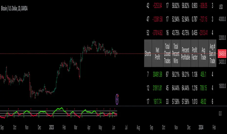
GKD-BT Multi-Ticker Full GKD Backtest [Loxx]The Giga Kaleidoscope GKD-BT Multi-Ticker Full GKD Backtest is a backtesting module included in Loxx's "Giga Kaleidoscope Modularized Trading System."
█ Giga Kaleidoscope GKD-BT Multi-Ticker Full GKD Backtest
The Multi-Ticker Full GKD Backtest is a Full GKD backtest that allows traders to test single GKD-C Confirmation indicator filtered by a GKD-B Multi-Ticker Baseline, GKD-V Volatility/Volume, and GKD-C Confirmation 2 indicator across 1-10 tickers. In addition. this module adds on various other long and short signls that fall outside the normal GKD standard long and short signals. These additional signals are formed using the GKD-B Multi-Ticker Baseline, GKD-V Volatility/Volume, GKD-C Confirmation 2, and GKD-C Continuation indicators. The purpose of this backtest is to enable traders to quickly evaluate a Baseline, Volatility/Volume, Confirmation 2, and Continuation indicators filtered GKD-C Confirmation 1 indicator across hundreds of tickers within 30-60 minutes.
The backtest module supports testing with 1 take profit and 1 stop loss. It also offers the option to limit testing to a specific date range, allowing simulated forward testing using historical data. This backtest module only includes standard long and short signals. Additionally, users can choose to display or hide a trading panel that provides relevant information about the backtest, statistics, and the current trade. Traders can also select a highlighting threshold for Total Percent Wins and Percent Profitable, and Profit Factor.
To use this indicator:
1. Import 1-10 tickers into the GKD-B Multi-Ticker Baseline indicator
2. Import the value "Input into NEW GKD-BT Multi-ticker Backtest" from the GKD-B Multi-Ticker Baseline indicator into the GKD-BT Multi-Ticker Full GKD Backtest.
3. Select the "Multi-ticker" option in the GKD-V Volatility/Volume indicator
4. Import 1-10 tickers into the GKD-V Volatility/Volume indicator
5. Import the value "Input into NEW GKD-BT Multi-ticker Backtest" from the GKD-V Volatility/Volume indicator into the GKD-BT Multi-Ticker Full GKD Backtest.
6. Select the "Multi-ticker" option in the GKD-C Confirmation 1 indicator.
7. Import 1-10 tickers into the GKD-C Confirmation 1 indicator.
8. Import the same 1-10 indicators into the GKD-BT Multi-Ticker Full GKD Backtest.
9. Import the value "Input into NEW GKD-BT Multi-ticker Backtest" from the GKD-C Confirmation 1 indicator into the GKD-BT Multi-Ticker Full GKD Backtest.
10. Import 1-10 tickers into the GKD-C Confirmation 2 indicator.
11. Import the same 1-10 indicators into the GKD-BT Multi-Ticker Full GKD Backtest.
12. Import the value "Input into NEW GKD-BT Multi-ticker Backtest" from the GKD-C Confirmation 2 indicator into the GKD-BT Multi-Ticker Full GKD Backtest.
13. Import 1-10 tickers into the GKD-C Continuation indicator.
14. Import the same 1-10 indicators into the GKD-BT Multi-Ticker Full GKD Backtest.
15. Import the value "Input into NEW GKD-BT Multi-ticker Backtest" from the GKD-C Continuation indicator into the GKD-BT Multi-Ticker Full GKD Backtest.
16. When importing tickers, ensure that you import the same type of tickers for all 1-10 tickers. For example, test only FX or Cryptocurrency or Stocks. Do not combine different tradable asset types.
17. Make sure that your chart is set to a ticker that corresponds to the tradable asset type. For cryptocurrency testing, set the chart to BTCUSDT. For Forex testing, set the chart to EURUSD.
This backtest includes the following metrics:
1. Net profit: Overall profit or loss achieved.
2. Total Closed Trades: Total number of closed trades, both winning and losing.
3. Total Percent Wins: Total wins, whether long or short, for the selected time interval regardless of commissions and other profit-modifying addons.
4. Percent Profitable: Total wins, whether long or short, that are also profitable, taking commissions into account.
5. Profit Factor: The ratio of gross profits to gross losses, indicating how much money the strategy made for every unit of money it lost.
6. Average Profit per Trade: The average gain or loss per trade, calculated by dividing the net profit by the total number of closed trades.
7. Average Number of Bars in Trade: The average number of bars that elapsed during trades for all closed trades.
Summary of notable settings:
Input Tickers separated by commas: Allows the user to input tickers separated by commas, specifying the symbols or tickers of financial instruments used in the backtest. The tickers should follow the format "EXCHANGE:TICKER" (e.g., "NASDAQ:AAPL, NYSE:MSFT").
Import GKD-B Baseline: Imports the "GKD-B Multi-Ticker Baseline" indicator.
Import GKD-V Volatility/Volume: Imports the "GKD-V Volatility/Volume" indicator.
Import GKD-C Confirmation: Imports the "GKD-C" indicator.
Activate Baseline: Activates the GKD-B Multi-Ticker Baseline.
Activate Goldie Locks Zone Minimum Threshold: Activates the inner Goldie Locks Zone from the GKD-B Multi-Ticker Baseline
Activate Goldie Locks Zone Maximum Threshold: Activates the outer Goldie Locks Zone from the GKD-B Multi-Ticker Baseline
Activate Volatility/Volume: Activates the GKD-V Volatility/Volume indicator.
Initial Capital: Represents the starting account balance for the backtest, denominated in the base currency of the trading account.
Order Size: Determines the quantity of contracts traded in each trade.
Order Type: Specifies the type of order used in the backtest, either "Contracts" or "% Equity."
Commission: Represents the commission per order or transaction cost incurred in each trade.
**the backtest data rendered to the chart above uses $5 commission per trade and 10% equity per trade with $1 million initial capital. Each backtest result for each ticker assumes these same inputs. The results are NOT cumulative, they are separate and isolate per ticker and trading side, long or short**
█ Volatility Types included
The GKD system utilizes volatility-based take profits and stop losses. Each take profit and stop loss is calculated as a multiple of volatility. You can change the values of the multipliers in the settings as well.
This module includes 17 types of volatility:
Close-to-Close
Parkinson
Garman-Klass
Rogers-Satchell
Yang-Zhang
Garman-Klass-Yang-Zhang
Exponential Weighted Moving Average
Standard Deviation of Log Returns
Pseudo GARCH(2,2)
Average True Range
True Range Double
Standard Deviation
Adaptive Deviation
Median Absolute Deviation
Efficiency-Ratio Adaptive ATR
Mean Absolute Deviation
Static Percent
Various volatility estimators and indicators that investors and traders can use to measure the dispersion or volatility of a financial instrument's price. Each estimator has its strengths and weaknesses, and the choice of estimator should depend on the specific needs and circumstances of the user.
Close-to-Close
Close-to-Close volatility is a classic and widely used volatility measure, sometimes referred to as historical volatility.
Volatility is an indicator of the speed of a stock price change. A stock with high volatility is one where the price changes rapidly and with a larger amplitude. The more volatile a stock is, the riskier it is.
Close-to-close historical volatility is calculated using only a stock's closing prices. It is the simplest volatility estimator. However, in many cases, it is not precise enough. Stock prices could jump significantly during a trading session and return to the opening value at the end. That means that a considerable amount of price information is not taken into account by close-to-close volatility.
Despite its drawbacks, Close-to-Close volatility is still useful in cases where the instrument doesn't have intraday prices. For example, mutual funds calculate their net asset values daily or weekly, and thus their prices are not suitable for more sophisticated volatility estimators.
Parkinson
Parkinson volatility is a volatility measure that uses the stock’s high and low price of the day.
The main difference between regular volatility and Parkinson volatility is that the latter uses high and low prices for a day, rather than only the closing price. This is useful as close-to-close prices could show little difference while large price movements could have occurred during the day. Thus, Parkinson's volatility is considered more precise and requires less data for calculation than close-to-close volatility.
One drawback of this estimator is that it doesn't take into account price movements after the market closes. Hence, it systematically undervalues volatility. This drawback is addressed in the Garman-Klass volatility estimator.
Garman-Klass
Garman-Klass is a volatility estimator that incorporates open, low, high, and close prices of a security.
Garman-Klass volatility extends Parkinson's volatility by taking into account the opening and closing prices. As markets are most active during the opening and closing of a trading session, it makes volatility estimation more accurate.
Garman and Klass also assumed that the process of price change follows a continuous diffusion process (Geometric Brownian motion). However, this assumption has several drawbacks. The method is not robust for opening jumps in price and trend movements.
Despite its drawbacks, the Garman-Klass estimator is still more effective than the basic formula since it takes into account not only the price at the beginning and end of the time interval but also intraday price extremes.
Researchers Rogers and Satchell have proposed a more efficient method for assessing historical volatility that takes into account price trends. See Rogers-Satchell Volatility for more detail.
Rogers-Satchell
Rogers-Satchell is an estimator for measuring the volatility of securities with an average return not equal to zero.
Unlike Parkinson and Garman-Klass estimators, Rogers-Satchell incorporates a drift term (mean return not equal to zero). As a result, it provides better volatility estimation when the underlying is trending.
The main disadvantage of this method is that it does not take into account price movements between trading sessions. This leads to an underestimation of volatility since price jumps periodically occur in the market precisely at the moments between sessions.
A more comprehensive estimator that also considers the gaps between sessions was developed based on the Rogers-Satchel formula in the 2000s by Yang-Zhang. See Yang Zhang Volatility for more detail.
Yang-Zhang
Yang Zhang is a historical volatility estimator that handles both opening jumps and the drift and has a minimum estimation error.
Yang-Zhang volatility can be thought of as a combination of the overnight (close-to-open volatility) and a weighted average of the Rogers-Satchell volatility and the day’s open-to-close volatility. It is considered to be 14 times more efficient than the close-to-close estimator.
Garman-Klass-Yang-Zhang
Garman-Klass-Yang-Zhang (GKYZ) volatility estimator incorporates the returns of open, high, low, and closing prices in its calculation.
GKYZ volatility estimator takes into account overnight jumps but not the trend, i.e., it assumes that the underlying asset follows a Geometric Brownian Motion (GBM) process with zero drift. Therefore, the GKYZ volatility estimator tends to overestimate the volatility when the drift is different from zero. However, for a GBM process, this estimator is eight times more efficient than the close-to-close volatility estimator.
Exponential Weighted Moving Average
The Exponentially Weighted Moving Average (EWMA) is a quantitative or statistical measure used to model or describe a time series. The EWMA is widely used in finance, with the main applications being technical analysis and volatility modeling.
The moving average is designed such that older observations are given lower weights. The weights decrease exponentially as the data point gets older – hence the name exponentially weighted.
The only decision a user of the EWMA must make is the parameter lambda. The parameter decides how important the current observation is in the calculation of the EWMA. The higher the value of lambda, the more closely the EWMA tracks the original time series.
Standard Deviation of Log Returns
This is the simplest calculation of volatility. It's the standard deviation of ln(close/close(1)).
Pseudo GARCH(2,2)
This is calculated using a short- and long-run mean of variance multiplied by ?.
?avg(var;M) + (1 ? ?) avg(var;N) = 2?var/(M+1-(M-1)L) + 2(1-?)var/(M+1-(M-1)L)
Solving for ? can be done by minimizing the mean squared error of estimation; that is, regressing L^-1var - avg(var; N) against avg(var; M) - avg(var; N) and using the resulting beta estimate as ?.
Average True Range
The average true range (ATR) is a technical analysis indicator, introduced by market technician J. Welles Wilder Jr. in his book New Concepts in Technical Trading Systems, that measures market volatility by decomposing the entire range of an asset price for that period.
The true range indicator is taken as the greatest of the following: current high less the current low; the absolute value of the current high less the previous close; and the absolute value of the current low less the previous close. The ATR is then a moving average, generally using 14 days, of the true ranges.
True Range Double
A special case of ATR that attempts to correct for volatility skew.
Standard Deviation
Standard deviation is a statistic that measures the dispersion of a dataset relative to its mean and is calculated as the square root of the variance. The standard deviation is calculated as the square root of variance by determining each data point's deviation relative to the mean. If the data points are further from the mean, there is a higher deviation within the data set; thus, the more spread out the data, the higher the standard deviation.
Adaptive Deviation
By definition, the Standard Deviation (STD, also represented by the Greek letter sigma ? or the Latin letter s) is a measure that is used to quantify the amount of variation or dispersion of a set of data values. In technical analysis, we usually use it to measure the level of current volatility.
Standard Deviation is based on Simple Moving Average calculation for mean value. This version of standard deviation uses the properties of EMA to calculate what can be called a new type of deviation, and since it is based on EMA, we can call it EMA deviation. Additionally, Perry Kaufman's efficiency ratio is used to make it adaptive (since all EMA type calculations are nearly perfect for adapting).
The difference when compared to the standard is significant--not just because of EMA usage, but the efficiency ratio makes it a "bit more logical" in very volatile market conditions.
Median Absolute Deviation
The median absolute deviation is a measure of statistical dispersion. Moreover, the MAD is a robust statistic, being more resilient to outliers in a data set than the standard deviation. In the standard deviation, the distances from the mean are squared, so large deviations are weighted more heavily, and thus outliers can heavily influence it. In the MAD, the deviations of a small number of outliers are irrelevant.
Because the MAD is a more robust estimator of scale than the sample variance or standard deviation, it works better with distributions without a mean or variance, such as the Cauchy distribution.
For this indicator, a manual recreation of the quantile function in Pine Script is used. This is so users have a full inside view into how this is calculated.
Efficiency-Ratio Adaptive ATR
Average True Range (ATR) is a widely used indicator for many occasions in technical analysis. It is calculated as the RMA of the true range. This version adds a "twist": it uses Perry Kaufman's Efficiency Ratio to calculate adaptive true range.
Mean Absolute Deviation
The mean absolute deviation (MAD) is a measure of variability that indicates the average distance between observations and their mean. MAD uses the original units of the data, which simplifies interpretation. Larger values signify that the data points spread out further from the average. Conversely, lower values correspond to data points bunching closer to it. The mean absolute deviation is also known as the mean deviation and average absolute deviation.
This definition of the mean absolute deviation sounds similar to the standard deviation (SD). While both measure variability, they have different calculations. In recent years, some proponents of MAD have suggested that it replace the SD as the primary measure because it is a simpler concept that better fits real life.
█ Giga Kaleidoscope Modularized Trading System
Core components of an NNFX algorithmic trading strategy
The NNFX algorithm is built on the principles of trend, momentum, and volatility. There are six core components in the NNFX trading algorithm:
1. Volatility - price volatility; e.g., Average True Range, True Range Double, Close-to-Close, etc.
2. Baseline - a moving average to identify price trend
3. Confirmation 1 - a technical indicator used to identify trends
4. Confirmation 2 - a technical indicator used to identify trends
5. Continuation - a technical indicator used to identify trends
6. Volatility/Volume - a technical indicator used to identify volatility/volume breakouts/breakdown
7. Exit - a technical indicator used to determine when a trend is exhausted
8. Metamorphosis - a technical indicator that produces a compound signal from the combination of other GKD indicators*
*(not part of the NNFX algorithm)
What is Volatility in the NNFX trading system?
In the NNFX (No Nonsense Forex) trading system, ATR (Average True Range) is typically used to measure the volatility of an asset. It is used as a part of the system to help determine the appropriate stop loss and take profit levels for a trade. ATR is calculated by taking the average of the true range values over a specified period.
True range is calculated as the maximum of the following values:
-Current high minus the current low
-Absolute value of the current high minus the previous close
-Absolute value of the current low minus the previous close
ATR is a dynamic indicator that changes with changes in volatility. As volatility increases, the value of ATR increases, and as volatility decreases, the value of ATR decreases. By using ATR in NNFX system, traders can adjust their stop loss and take profit levels according to the volatility of the asset being traded. This helps to ensure that the trade is given enough room to move, while also minimizing potential losses.
Other types of volatility include True Range Double (TRD), Close-to-Close, and Garman-Klass
What is a Baseline indicator?
The baseline is essentially a moving average, and is used to determine the overall direction of the market.
The baseline in the NNFX system is used to filter out trades that are not in line with the long-term trend of the market. The baseline is plotted on the chart along with other indicators, such as the Moving Average (MA), the Relative Strength Index (RSI), and the Average True Range (ATR).
Trades are only taken when the price is in the same direction as the baseline. For example, if the baseline is sloping upwards, only long trades are taken, and if the baseline is sloping downwards, only short trades are taken. This approach helps to ensure that trades are in line with the overall trend of the market, and reduces the risk of entering trades that are likely to fail.
By using a baseline in the NNFX system, traders can have a clear reference point for determining the overall trend of the market, and can make more informed trading decisions. The baseline helps to filter out noise and false signals, and ensures that trades are taken in the direction of the long-term trend.
What is a Confirmation indicator?
Confirmation indicators are technical indicators that are used to confirm the signals generated by primary indicators. Primary indicators are the core indicators used in the NNFX system, such as the Average True Range (ATR), the Moving Average (MA), and the Relative Strength Index (RSI).
The purpose of the confirmation indicators is to reduce false signals and improve the accuracy of the trading system. They are designed to confirm the signals generated by the primary indicators by providing additional information about the strength and direction of the trend.
Some examples of confirmation indicators that may be used in the NNFX system include the Bollinger Bands, the MACD (Moving Average Convergence Divergence), and the MACD Oscillator. These indicators can provide information about the volatility, momentum, and trend strength of the market, and can be used to confirm the signals generated by the primary indicators.
In the NNFX system, confirmation indicators are used in combination with primary indicators and other filters to create a trading system that is robust and reliable. By using multiple indicators to confirm trading signals, the system aims to reduce the risk of false signals and improve the overall profitability of the trades.
What is a Continuation indicator?
In the NNFX (No Nonsense Forex) trading system, a continuation indicator is a technical indicator that is used to confirm a current trend and predict that the trend is likely to continue in the same direction. A continuation indicator is typically used in conjunction with other indicators in the system, such as a baseline indicator, to provide a comprehensive trading strategy.
What is a Volatility/Volume indicator?
Volume indicators, such as the On Balance Volume (OBV), the Chaikin Money Flow (CMF), or the Volume Price Trend (VPT), are used to measure the amount of buying and selling activity in a market. They are based on the trading volume of the market, and can provide information about the strength of the trend. In the NNFX system, volume indicators are used to confirm trading signals generated by the Moving Average and the Relative Strength Index. Volatility indicators include Average Direction Index, Waddah Attar, and Volatility Ratio. In the NNFX trading system, volatility is a proxy for volume and vice versa.
By using volume indicators as confirmation tools, the NNFX trading system aims to reduce the risk of false signals and improve the overall profitability of trades. These indicators can provide additional information about the market that is not captured by the primary indicators, and can help traders to make more informed trading decisions. In addition, volume indicators can be used to identify potential changes in market trends and to confirm the strength of price movements.
What is an Exit indicator?
The exit indicator is used in conjunction with other indicators in the system, such as the Moving Average (MA), the Relative Strength Index (RSI), and the Average True Range (ATR), to provide a comprehensive trading strategy.
The exit indicator in the NNFX system can be any technical indicator that is deemed effective at identifying optimal exit points. Examples of exit indicators that are commonly used include the Parabolic SAR, the Average Directional Index (ADX), and the Chandelier Exit.
The purpose of the exit indicator is to identify when a trend is likely to reverse or when the market conditions have changed, signaling the need to exit a trade. By using an exit indicator, traders can manage their risk and prevent significant losses.
In the NNFX system, the exit indicator is used in conjunction with a stop loss and a take profit order to maximize profits and minimize losses. The stop loss order is used to limit the amount of loss that can be incurred if the trade goes against the trader, while the take profit order is used to lock in profits when the trade is moving in the trader's favor.
Overall, the use of an exit indicator in the NNFX trading system is an important component of a comprehensive trading strategy. It allows traders to manage their risk effectively and improve the profitability of their trades by exiting at the right time.
What is an Metamorphosis indicator?
The concept of a metamorphosis indicator involves the integration of two or more GKD indicators to generate a compound signal. This is achieved by evaluating the accuracy of each indicator and selecting the signal from the indicator with the highest accuracy. As an illustration, let's consider a scenario where we calculate the accuracy of 10 indicators and choose the signal from the indicator that demonstrates the highest accuracy.
The resulting output from the metamorphosis indicator can then be utilized in a GKD-BT backtest by occupying a slot that aligns with the purpose of the metamorphosis indicator. The slot can be a GKD-B, GKD-C, or GKD-E slot, depending on the specific requirements and objectives of the indicator. This allows for seamless integration and utilization of the compound signal within the GKD-BT framework.
How does Loxx's GKD (Giga Kaleidoscope Modularized Trading System) implement the NNFX algorithm outlined above?
Loxx's GKD v2.0 system has five types of modules (indicators/strategies). These modules are:
1. GKD-BT - Backtesting module (Volatility, Number 1 in the NNFX algorithm)
2. GKD-B - Baseline module (Baseline and Volatility/Volume, Numbers 1 and 2 in the NNFX algorithm)
3. GKD-C - Confirmation 1/2 and Continuation module (Confirmation 1/2 and Continuation, Numbers 3, 4, and 5 in the NNFX algorithm)
4. GKD-V - Volatility/Volume module (Confirmation 1/2, Number 6 in the NNFX algorithm)
5. GKD-E - Exit module (Exit, Number 7 in the NNFX algorithm)
6. GKD-M - Metamorphosis module (Metamorphosis, Number 8 in the NNFX algorithm, but not part of the NNFX algorithm)
(additional module types will added in future releases)
Each module interacts with every module by passing data to A backtest module wherein the various components of the GKD system are combined to create a trading signal.
That is, the Baseline indicator passes its data to Volatility/Volume. The Volatility/Volume indicator passes its values to the Confirmation 1 indicator. The Confirmation 1 indicator passes its values to the Confirmation 2 indicator. The Confirmation 2 indicator passes its values to the Continuation indicator. The Continuation indicator passes its values to the Exit indicator, and finally, the Exit indicator passes its values to the Backtest strategy.
This chaining of indicators requires that each module conform to Loxx's GKD protocol, therefore allowing for the testing of every possible combination of technical indicators that make up the six components of the NNFX algorithm.
What does the application of the GKD trading system look like?
Example trading system:
Backtest: Multi-Ticker Full GKD Backtest as shown on the chart above
Baseline: Hull Moving Average as shown on the chart above
Volatility/Volume: Hurst Exponent as shown on the chart above
Confirmation 1: Fisher Transform as shown on the chart above
Confirmation 2: uf2018 as shown on the chart above
Continuation: Coppock Curve as shown on the chart above
Exit: Rex Oscillator
Metamorphosis: Baseline Optimizer
Each GKD indicator is denoted with a module identifier of either: GKD-BT, GKD-B, GKD-C, GKD-V, GKD-M, or GKD-E. This allows traders to understand to which module each indicator belongs and where each indicator fits into the GKD system.
█ Giga Kaleidoscope Modularized Trading System Signals
Standard Entry
1. GKD-C Confirmation gives signal
2. Baseline agrees
3. Price inside Goldie Locks Zone Minimum
4. Price inside Goldie Locks Zone Maximum
5. Confirmation 2 agrees
6. Volatility/Volume agrees
1-Candle Standard Entry
1a. GKD-C Confirmation gives signal
2a. Baseline agrees
3a. Price inside Goldie Locks Zone Minimum
4a. Price inside Goldie Locks Zone Maximum
Next Candle
1b. Price retraced
2b. Baseline agrees
3b. Confirmation 1 agrees
4b. Confirmation 2 agrees
5b. Volatility/Volume agrees
Baseline Entry
1. GKD-B Basline gives signal
2. Confirmation 1 agrees
3. Price inside Goldie Locks Zone Minimum
4. Price inside Goldie Locks Zone Maximum
5. Confirmation 2 agrees
6. Volatility/Volume agrees
7. Confirmation 1 signal was less than 'Maximum Allowable PSBC Bars Back' prior
1-Candle Baseline Entry
1a. GKD-B Baseline gives signal
2a. Confirmation 1 agrees
3a. Price inside Goldie Locks Zone Minimum
4a. Price inside Goldie Locks Zone Maximum
5a. Confirmation 1 signal was less than 'Maximum Allowable PSBC Bars Back' prior
Next Candle
1b. Price retraced
2b. Baseline agrees
3b. Confirmation 1 agrees
4b. Confirmation 2 agrees
5b. Volatility/Volume agrees
Volatility/Volume Entry
1. GKD-V Volatility/Volume gives signal
2. Confirmation 1 agrees
3. Price inside Goldie Locks Zone Minimum
4. Price inside Goldie Locks Zone Maximum
5. Confirmation 2 agrees
6. Baseline agrees
7. Confirmation 1 signal was less than 7 candles prior
1-Candle Volatility/Volume Entry
1a. GKD-V Volatility/Volume gives signal
2a. Confirmation 1 agrees
3a. Price inside Goldie Locks Zone Minimum
4a. Price inside Goldie Locks Zone Maximum
5a. Confirmation 1 signal was less than 'Maximum Allowable PSVVC Bars Back' prior
Next Candle
1b. Price retraced
2b. Volatility/Volume agrees
3b. Confirmation 1 agrees
4b. Confirmation 2 agrees
5b. Baseline agrees
Confirmation 2 Entry
1. GKD-C Confirmation 2 gives signal
2. Confirmation 1 agrees
3. Price inside Goldie Locks Zone Minimum
4. Price inside Goldie Locks Zone Maximum
5. Volatility/Volume agrees
6. Baseline agrees
7. Confirmation 1 signal was less than 7 candles prior
1-Candle Confirmation 2 Entry
1a. GKD-C Confirmation 2 gives signal
2a. Confirmation 1 agrees
3a. Price inside Goldie Locks Zone Minimum
4a. Price inside Goldie Locks Zone Maximum
5a. Confirmation 1 signal was less than 'Maximum Allowable PSC2C Bars Back' prior
Next Candle
1b. Price retraced
2b. Confirmation 2 agrees
3b. Confirmation 1 agrees
4b. Volatility/Volume agrees
5b. Baseline agrees
PullBack Entry
1a. GKD-B Baseline gives signal
2a. Confirmation 1 agrees
3a. Price is beyond 1.0x Volatility of Baseline
Next Candle
1b. Price inside Goldie Locks Zone Minimum
2b. Price inside Goldie Locks Zone Maximum
3b. Confirmation 1 agrees
4b. Confirmation 2 agrees
5b. Volatility/Volume agrees
Continuation Entry
1. Standard Entry, 1-Candle Standard Entry, Baseline Entry, 1-Candle Baseline Entry, Volatility/Volume Entry, 1-Candle Volatility/Volume Entry, Confirmation 2 Entry, 1-Candle Confirmation 2 Entry, or Pullback entry triggered previously
2. Baseline hasn't crossed since entry signal trigger
4. Confirmation 1 agrees
5. Baseline agrees
6. Confirmation 2 agrees
█ Connecting to Backtests
All GKD indicators are chained indicators meaning you export the value of the indicators to specialized backtest to creat your GKD trading system. Each indicator contains a proprietary signal generation algo that will only work with GKD backtests. You can find these backtests using the links below.
GKD-BT Giga Confirmation Stack Backtest
GKD-BT Giga Stacks Backtest
GKD-BT Full Giga Kaleidoscope Backtest
GKD-BT Solo Confirmation Super Complex Backtest
GKD-BT Solo Confirmation Complex Backtest
GKD-BT Solo Confirmation Simple Backtest
GKD-M Baseline Optimizer
GKD-M Accuracy Alchemist
GKD-BT Multi-Ticker SCC Backtest
GKD-BT Multi-Ticker SCS Backtest
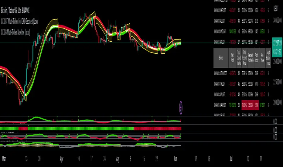
GKD-BT Multi-Ticker SCSC Backtest [Loxx]The Giga Kaleidoscope GKD-BT Multi-Ticker SCSC Backtest is a backtesting module included in Loxx's "Giga Kaleidoscope Modularized Trading System."
█ Giga Kaleidoscope GKD-BT Multi-Ticker SCSC Backtest
The Multi-Ticker SCSC Backtest is a Solo Confirmation Super Complex backtest that allows traders to test single GKD-C Confirmation indicator filtered by both a GKD-B Multi-Ticker Baseline and GKD-V Volatility/Volume indicator across 1-10 tickers. In addition. this module adds on various other long and short signls that fall outside the normal GKD standard long and short signals. These additional signals are formed using the GKD-B Multi-Ticker Baseline, GKD-V Volatility/Volume, and GKD-C Continuation indicators. The purpose of this backtest is to enable traders to quickly evaluate a Baseline, Volatility/Volume, and Continuation indicators filtered GKD-C Confirmation 1 indicator across hundreds of tickers within 30-60 minutes.
The backtest module supports testing with 1 take profit and 1 stop loss. It also offers the option to limit testing to a specific date range, allowing simulated forward testing using historical data. This backtest module only includes standard long and short signals. Additionally, users can choose to display or hide a trading panel that provides relevant information about the backtest, statistics, and the current trade. Traders can also select a highlighting threshold for Total Percent Wins and Percent Profitable, and Profit Factor.
To use this indicator:
1. Import 1-10 tickers into the GKD-B Multi-Ticker Baseline indicator
2. Import the value "Input into NEW GKD-BT Multi-ticker Backtest" from the GKD-B Multi-Ticker Baseline indicator into the GKD-BT Multi-Ticker SCSC Backtest.
3. Select the "Multi-ticker" option in the GKD-V Volatility/Volume indicator
4. Import 1-10 tickers into the GKD-V Volatility/Volume indicator
5. Import the value "Input into NEW GKD-BT Multi-ticker Backtest" from the GKD-V Volatility/Volume indicator into the GKD-BT Multi-Ticker SCSC Backtest.
6. Select the "Multi-ticker" option in the GKD-C Confirmation indicator.
7. Import 1-10 tickers into the GKD-C Confirmation indicator.
8. Import the same 1-10 indicators into the GKD-BT Multi-Ticker SCSC Backtest.
9. Import the value "Input into NEW GKD-BT Multi-ticker Backtest" from the GKD-C Confirmation indicator into the GKD-BT Multi-Ticker SCSC Backtest.
10. Import 1-10 tickers into the GKD-C Continuation indicator.
11. Import the same 1-10 indicators into the GKD-BT Multi-Ticker SCSC Backtest.
12. Import the value "Input into NEW GKD-BT Multi-ticker Backtest" from the GKD-C Continuation indicator into the GKD-BT Multi-Ticker SCSC Backtest.
13. When importing tickers, ensure that you import the same type of tickers for all 1-10 tickers. For example, test only FX or Cryptocurrency or Stocks. Do not combine different tradable asset types.
14. Make sure that your chart is set to a ticker that corresponds to the tradable asset type. For cryptocurrency testing, set the chart to BTCUSDT. For Forex testing, set the chart to EURUSD.
This backtest includes the following metrics:
1. Net profit: Overall profit or loss achieved.
2. Total Closed Trades: Total number of closed trades, both winning and losing.
3. Total Percent Wins: Total wins, whether long or short, for the selected time interval regardless of commissions and other profit-modifying addons.
4. Percent Profitable: Total wins, whether long or short, that are also profitable, taking commissions into account.
5. Profit Factor: The ratio of gross profits to gross losses, indicating how much money the strategy made for every unit of money it lost.
6. Average Profit per Trade: The average gain or loss per trade, calculated by dividing the net profit by the total number of closed trades.
7. Average Number of Bars in Trade: The average number of bars that elapsed during trades for all closed trades.
Summary of notable settings:
Input Tickers separated by commas: Allows the user to input tickers separated by commas, specifying the symbols or tickers of financial instruments used in the backtest. The tickers should follow the format "EXCHANGE:TICKER" (e.g., "NASDAQ:AAPL, NYSE:MSFT").
Import GKD-B Baseline: Imports the "GKD-B Multi-Ticker Baseline" indicator.
Import GKD-V Volatility/Volume: Imports the "GKD-V Volatility/Volume" indicator.
Import GKD-C Confirmation: Imports the "GKD-C Confirmation" indicator.
Import GKD-C Continuation: Imports the "GKD-C Continuation" indicator.
Initial Capital: Represents the starting account balance for the backtest, denominated in the base currency of the trading account.
Order Size: Determines the quantity of contracts traded in each trade.
Order Type: Specifies the type of order used in the backtest, either "Contracts" or "% Equity."
Commission: Represents the commission per order or transaction cost incurred in each trade.
**the backtest data rendered to the chart above uses $5 commission per trade and 10% equity per trade with $1 million initial capital. Each backtest result for each ticker assumes these same inputs. The results are NOT cumulative, they are separate and isolate per ticker and trading side, long or short**
█ Volatility Types included
The GKD system utilizes volatility-based take profits and stop losses. Each take profit and stop loss is calculated as a multiple of volatility. You can change the values of the multipliers in the settings as well.
This module includes 17 types of volatility:
Close-to-Close
Parkinson
Garman-Klass
Rogers-Satchell
Yang-Zhang
Garman-Klass-Yang-Zhang
Exponential Weighted Moving Average
Standard Deviation of Log Returns
Pseudo GARCH(2,2)
Average True Range
True Range Double
Standard Deviation
Adaptive Deviation
Median Absolute Deviation
Efficiency-Ratio Adaptive ATR
Mean Absolute Deviation
Static Percent
Various volatility estimators and indicators that investors and traders can use to measure the dispersion or volatility of a financial instrument's price. Each estimator has its strengths and weaknesses, and the choice of estimator should depend on the specific needs and circumstances of the user.
Close-to-Close
Close-to-Close volatility is a classic and widely used volatility measure, sometimes referred to as historical volatility.
Volatility is an indicator of the speed of a stock price change. A stock with high volatility is one where the price changes rapidly and with a larger amplitude. The more volatile a stock is, the riskier it is.
Close-to-close historical volatility is calculated using only a stock's closing prices. It is the simplest volatility estimator. However, in many cases, it is not precise enough. Stock prices could jump significantly during a trading session and return to the opening value at the end. That means that a considerable amount of price information is not taken into account by close-to-close volatility.
Despite its drawbacks, Close-to-Close volatility is still useful in cases where the instrument doesn't have intraday prices. For example, mutual funds calculate their net asset values daily or weekly, and thus their prices are not suitable for more sophisticated volatility estimators.
Parkinson
Parkinson volatility is a volatility measure that uses the stock’s high and low price of the day.
The main difference between regular volatility and Parkinson volatility is that the latter uses high and low prices for a day, rather than only the closing price. This is useful as close-to-close prices could show little difference while large price movements could have occurred during the day. Thus, Parkinson's volatility is considered more precise and requires less data for calculation than close-to-close volatility.
One drawback of this estimator is that it doesn't take into account price movements after the market closes. Hence, it systematically undervalues volatility. This drawback is addressed in the Garman-Klass volatility estimator.
Garman-Klass
Garman-Klass is a volatility estimator that incorporates open, low, high, and close prices of a security.
Garman-Klass volatility extends Parkinson's volatility by taking into account the opening and closing prices. As markets are most active during the opening and closing of a trading session, it makes volatility estimation more accurate.
Garman and Klass also assumed that the process of price change follows a continuous diffusion process (Geometric Brownian motion). However, this assumption has several drawbacks. The method is not robust for opening jumps in price and trend movements.
Despite its drawbacks, the Garman-Klass estimator is still more effective than the basic formula since it takes into account not only the price at the beginning and end of the time interval but also intraday price extremes.
Researchers Rogers and Satchell have proposed a more efficient method for assessing historical volatility that takes into account price trends. See Rogers-Satchell Volatility for more detail.
Rogers-Satchell
Rogers-Satchell is an estimator for measuring the volatility of securities with an average return not equal to zero.
Unlike Parkinson and Garman-Klass estimators, Rogers-Satchell incorporates a drift term (mean return not equal to zero). As a result, it provides better volatility estimation when the underlying is trending.
The main disadvantage of this method is that it does not take into account price movements between trading sessions. This leads to an underestimation of volatility since price jumps periodically occur in the market precisely at the moments between sessions.
A more comprehensive estimator that also considers the gaps between sessions was developed based on the Rogers-Satchel formula in the 2000s by Yang-Zhang. See Yang Zhang Volatility for more detail.
Yang-Zhang
Yang Zhang is a historical volatility estimator that handles both opening jumps and the drift and has a minimum estimation error.
Yang-Zhang volatility can be thought of as a combination of the overnight (close-to-open volatility) and a weighted average of the Rogers-Satchell volatility and the day’s open-to-close volatility. It is considered to be 14 times more efficient than the close-to-close estimator.
Garman-Klass-Yang-Zhang
Garman-Klass-Yang-Zhang (GKYZ) volatility estimator incorporates the returns of open, high, low, and closing prices in its calculation.
GKYZ volatility estimator takes into account overnight jumps but not the trend, i.e., it assumes that the underlying asset follows a Geometric Brownian Motion (GBM) process with zero drift. Therefore, the GKYZ volatility estimator tends to overestimate the volatility when the drift is different from zero. However, for a GBM process, this estimator is eight times more efficient than the close-to-close volatility estimator.
Exponential Weighted Moving Average
The Exponentially Weighted Moving Average (EWMA) is a quantitative or statistical measure used to model or describe a time series. The EWMA is widely used in finance, with the main applications being technical analysis and volatility modeling.
The moving average is designed such that older observations are given lower weights. The weights decrease exponentially as the data point gets older – hence the name exponentially weighted.
The only decision a user of the EWMA must make is the parameter lambda. The parameter decides how important the current observation is in the calculation of the EWMA. The higher the value of lambda, the more closely the EWMA tracks the original time series.
Standard Deviation of Log Returns
This is the simplest calculation of volatility. It's the standard deviation of ln(close/close(1)).
Pseudo GARCH(2,2)
This is calculated using a short- and long-run mean of variance multiplied by ?.
?avg(var;M) + (1 ? ?) avg(var;N) = 2?var/(M+1-(M-1)L) + 2(1-?)var/(M+1-(M-1)L)
Solving for ? can be done by minimizing the mean squared error of estimation; that is, regressing L^-1var - avg(var; N) against avg(var; M) - avg(var; N) and using the resulting beta estimate as ?.
Average True Range
The average true range (ATR) is a technical analysis indicator, introduced by market technician J. Welles Wilder Jr. in his book New Concepts in Technical Trading Systems, that measures market volatility by decomposing the entire range of an asset price for that period.
The true range indicator is taken as the greatest of the following: current high less the current low; the absolute value of the current high less the previous close; and the absolute value of the current low less the previous close. The ATR is then a moving average, generally using 14 days, of the true ranges.
True Range Double
A special case of ATR that attempts to correct for volatility skew.
Standard Deviation
Standard deviation is a statistic that measures the dispersion of a dataset relative to its mean and is calculated as the square root of the variance. The standard deviation is calculated as the square root of variance by determining each data point's deviation relative to the mean. If the data points are further from the mean, there is a higher deviation within the data set; thus, the more spread out the data, the higher the standard deviation.
Adaptive Deviation
By definition, the Standard Deviation (STD, also represented by the Greek letter sigma ? or the Latin letter s) is a measure that is used to quantify the amount of variation or dispersion of a set of data values. In technical analysis, we usually use it to measure the level of current volatility.
Standard Deviation is based on Simple Moving Average calculation for mean value. This version of standard deviation uses the properties of EMA to calculate what can be called a new type of deviation, and since it is based on EMA, we can call it EMA deviation. Additionally, Perry Kaufman's efficiency ratio is used to make it adaptive (since all EMA type calculations are nearly perfect for adapting).
The difference when compared to the standard is significant--not just because of EMA usage, but the efficiency ratio makes it a "bit more logical" in very volatile market conditions.
Median Absolute Deviation
The median absolute deviation is a measure of statistical dispersion. Moreover, the MAD is a robust statistic, being more resilient to outliers in a data set than the standard deviation. In the standard deviation, the distances from the mean are squared, so large deviations are weighted more heavily, and thus outliers can heavily influence it. In the MAD, the deviations of a small number of outliers are irrelevant.
Because the MAD is a more robust estimator of scale than the sample variance or standard deviation, it works better with distributions without a mean or variance, such as the Cauchy distribution.
For this indicator, a manual recreation of the quantile function in Pine Script is used. This is so users have a full inside view into how this is calculated.
Efficiency-Ratio Adaptive ATR
Average True Range (ATR) is a widely used indicator for many occasions in technical analysis. It is calculated as the RMA of the true range. This version adds a "twist": it uses Perry Kaufman's Efficiency Ratio to calculate adaptive true range.
Mean Absolute Deviation
The mean absolute deviation (MAD) is a measure of variability that indicates the average distance between observations and their mean. MAD uses the original units of the data, which simplifies interpretation. Larger values signify that the data points spread out further from the average. Conversely, lower values correspond to data points bunching closer to it. The mean absolute deviation is also known as the mean deviation and average absolute deviation.
This definition of the mean absolute deviation sounds similar to the standard deviation (SD). While both measure variability, they have different calculations. In recent years, some proponents of MAD have suggested that it replace the SD as the primary measure because it is a simpler concept that better fits real life.
█ Giga Kaleidoscope Modularized Trading System
Core components of an NNFX algorithmic trading strategy
The NNFX algorithm is built on the principles of trend, momentum, and volatility. There are six core components in the NNFX trading algorithm:
1. Volatility - price volatility; e.g., Average True Range, True Range Double, Close-to-Close, etc.
2. Baseline - a moving average to identify price trend
3. Confirmation 1 - a technical indicator used to identify trends
4. Confirmation 2 - a technical indicator used to identify trends
5. Continuation - a technical indicator used to identify trends
6. Volatility/Volume - a technical indicator used to identify volatility/volume breakouts/breakdown
7. Exit - a technical indicator used to determine when a trend is exhausted
8. Metamorphosis - a technical indicator that produces a compound signal from the combination of other GKD indicators*
*(not part of the NNFX algorithm)
What is Volatility in the NNFX trading system?
In the NNFX (No Nonsense Forex) trading system, ATR (Average True Range) is typically used to measure the volatility of an asset. It is used as a part of the system to help determine the appropriate stop loss and take profit levels for a trade. ATR is calculated by taking the average of the true range values over a specified period.
True range is calculated as the maximum of the following values:
-Current high minus the current low
-Absolute value of the current high minus the previous close
-Absolute value of the current low minus the previous close
ATR is a dynamic indicator that changes with changes in volatility. As volatility increases, the value of ATR increases, and as volatility decreases, the value of ATR decreases. By using ATR in NNFX system, traders can adjust their stop loss and take profit levels according to the volatility of the asset being traded. This helps to ensure that the trade is given enough room to move, while also minimizing potential losses.
Other types of volatility include True Range Double (TRD), Close-to-Close, and Garman-Klass
What is a Baseline indicator?
The baseline is essentially a moving average, and is used to determine the overall direction of the market.
The baseline in the NNFX system is used to filter out trades that are not in line with the long-term trend of the market. The baseline is plotted on the chart along with other indicators, such as the Moving Average (MA), the Relative Strength Index (RSI), and the Average True Range (ATR).
Trades are only taken when the price is in the same direction as the baseline. For example, if the baseline is sloping upwards, only long trades are taken, and if the baseline is sloping downwards, only short trades are taken. This approach helps to ensure that trades are in line with the overall trend of the market, and reduces the risk of entering trades that are likely to fail.
By using a baseline in the NNFX system, traders can have a clear reference point for determining the overall trend of the market, and can make more informed trading decisions. The baseline helps to filter out noise and false signals, and ensures that trades are taken in the direction of the long-term trend.
What is a Confirmation indicator?
Confirmation indicators are technical indicators that are used to confirm the signals generated by primary indicators. Primary indicators are the core indicators used in the NNFX system, such as the Average True Range (ATR), the Moving Average (MA), and the Relative Strength Index (RSI).
The purpose of the confirmation indicators is to reduce false signals and improve the accuracy of the trading system. They are designed to confirm the signals generated by the primary indicators by providing additional information about the strength and direction of the trend.
Some examples of confirmation indicators that may be used in the NNFX system include the Bollinger Bands, the MACD (Moving Average Convergence Divergence), and the MACD Oscillator. These indicators can provide information about the volatility, momentum, and trend strength of the market, and can be used to confirm the signals generated by the primary indicators.
In the NNFX system, confirmation indicators are used in combination with primary indicators and other filters to create a trading system that is robust and reliable. By using multiple indicators to confirm trading signals, the system aims to reduce the risk of false signals and improve the overall profitability of the trades.
What is a Continuation indicator?
In the NNFX (No Nonsense Forex) trading system, a continuation indicator is a technical indicator that is used to confirm a current trend and predict that the trend is likely to continue in the same direction. A continuation indicator is typically used in conjunction with other indicators in the system, such as a baseline indicator, to provide a comprehensive trading strategy.
What is a Volatility/Volume indicator?
Volume indicators, such as the On Balance Volume (OBV), the Chaikin Money Flow (CMF), or the Volume Price Trend (VPT), are used to measure the amount of buying and selling activity in a market. They are based on the trading volume of the market, and can provide information about the strength of the trend. In the NNFX system, volume indicators are used to confirm trading signals generated by the Moving Average and the Relative Strength Index. Volatility indicators include Average Direction Index, Waddah Attar, and Volatility Ratio. In the NNFX trading system, volatility is a proxy for volume and vice versa.
By using volume indicators as confirmation tools, the NNFX trading system aims to reduce the risk of false signals and improve the overall profitability of trades. These indicators can provide additional information about the market that is not captured by the primary indicators, and can help traders to make more informed trading decisions. In addition, volume indicators can be used to identify potential changes in market trends and to confirm the strength of price movements.
What is an Exit indicator?
The exit indicator is used in conjunction with other indicators in the system, such as the Moving Average (MA), the Relative Strength Index (RSI), and the Average True Range (ATR), to provide a comprehensive trading strategy.
The exit indicator in the NNFX system can be any technical indicator that is deemed effective at identifying optimal exit points. Examples of exit indicators that are commonly used include the Parabolic SAR, the Average Directional Index (ADX), and the Chandelier Exit.
The purpose of the exit indicator is to identify when a trend is likely to reverse or when the market conditions have changed, signaling the need to exit a trade. By using an exit indicator, traders can manage their risk and prevent significant losses.
In the NNFX system, the exit indicator is used in conjunction with a stop loss and a take profit order to maximize profits and minimize losses. The stop loss order is used to limit the amount of loss that can be incurred if the trade goes against the trader, while the take profit order is used to lock in profits when the trade is moving in the trader's favor.
Overall, the use of an exit indicator in the NNFX trading system is an important component of a comprehensive trading strategy. It allows traders to manage their risk effectively and improve the profitability of their trades by exiting at the right time.
What is an Metamorphosis indicator?
The concept of a metamorphosis indicator involves the integration of two or more GKD indicators to generate a compound signal. This is achieved by evaluating the accuracy of each indicator and selecting the signal from the indicator with the highest accuracy. As an illustration, let's consider a scenario where we calculate the accuracy of 10 indicators and choose the signal from the indicator that demonstrates the highest accuracy.
The resulting output from the metamorphosis indicator can then be utilized in a GKD-BT backtest by occupying a slot that aligns with the purpose of the metamorphosis indicator. The slot can be a GKD-B, GKD-C, or GKD-E slot, depending on the specific requirements and objectives of the indicator. This allows for seamless integration and utilization of the compound signal within the GKD-BT framework.
How does Loxx's GKD (Giga Kaleidoscope Modularized Trading System) implement the NNFX algorithm outlined above?
Loxx's GKD v2.0 system has five types of modules (indicators/strategies). These modules are:
1. GKD-BT - Backtesting module (Volatility, Number 1 in the NNFX algorithm)
2. GKD-B - Baseline module (Baseline and Volatility/Volume, Numbers 1 and 2 in the NNFX algorithm)
3. GKD-C - Confirmation 1/2 and Continuation module (Confirmation 1/2 and Continuation, Numbers 3, 4, and 5 in the NNFX algorithm)
4. GKD-V - Volatility/Volume module (Confirmation 1/2, Number 6 in the NNFX algorithm)
5. GKD-E - Exit module (Exit, Number 7 in the NNFX algorithm)
6. GKD-M - Metamorphosis module (Metamorphosis, Number 8 in the NNFX algorithm, but not part of the NNFX algorithm)
(additional module types will added in future releases)
Each module interacts with every module by passing data to A backtest module wherein the various components of the GKD system are combined to create a trading signal.
That is, the Baseline indicator passes its data to Volatility/Volume. The Volatility/Volume indicator passes its values to the Confirmation 1 indicator. The Confirmation 1 indicator passes its values to the Confirmation 2 indicator. The Confirmation 2 indicator passes its values to the Continuation indicator. The Continuation indicator passes its values to the Exit indicator, and finally, the Exit indicator passes its values to the Backtest strategy.
This chaining of indicators requires that each module conform to Loxx's GKD protocol, therefore allowing for the testing of every possible combination of technical indicators that make up the six components of the NNFX algorithm.
What does the application of the GKD trading system look like?
Example trading system:
Backtest: Multi-Ticker SCSC Backtest as shown on the chart above
Baseline: Hull Moving Average as shown on the chart above
Volatility/Volume: Hurst Exponent as shown on the chart above
Confirmation 1: Fisher Transform as shown on the chart above
Confirmation 2: uf2018
Continuation: Coppock Curve as shown on the chart above
Exit: Rex Oscillator
Metamorphosis: Baseline Optimizer
Each GKD indicator is denoted with a module identifier of either: GKD-BT, GKD-B, GKD-C, GKD-V, GKD-M, or GKD-E. This allows traders to understand to which module each indicator belongs and where each indicator fits into the GKD system.
█ Giga Kaleidoscope Modularized Trading System Signals
Standard Entry
1. GKD-C Confirmation gives signal
2. Baseline agrees
3. Price inside Goldie Locks Zone Minimum
4. Price inside Goldie Locks Zone Maximum
5. Confirmation 2 agrees
6. Volatility/Volume agrees
1-Candle Standard Entry
1a. GKD-C Confirmation gives signal
2a. Baseline agrees
3a. Price inside Goldie Locks Zone Minimum
4a. Price inside Goldie Locks Zone Maximum
Next Candle
1b. Price retraced
2b. Baseline agrees
3b. Confirmation 1 agrees
4b. Confirmation 2 agrees
5b. Volatility/Volume agrees
Baseline Entry
1. GKD-B Basline gives signal
2. Confirmation 1 agrees
3. Price inside Goldie Locks Zone Minimum
4. Price inside Goldie Locks Zone Maximum
5. Confirmation 2 agrees
6. Volatility/Volume agrees
7. Confirmation 1 signal was less than 'Maximum Allowable PSBC Bars Back' prior
1-Candle Baseline Entry
1a. GKD-B Baseline gives signal
2a. Confirmation 1 agrees
3a. Price inside Goldie Locks Zone Minimum
4a. Price inside Goldie Locks Zone Maximum
5a. Confirmation 1 signal was less than 'Maximum Allowable PSBC Bars Back' prior
Next Candle
1b. Price retraced
2b. Baseline agrees
3b. Confirmation 1 agrees
4b. Confirmation 2 agrees
5b. Volatility/Volume agrees
Volatility/Volume Entry
1. GKD-V Volatility/Volume gives signal
2. Confirmation 1 agrees
3. Price inside Goldie Locks Zone Minimum
4. Price inside Goldie Locks Zone Maximum
5. Confirmation 2 agrees
6. Baseline agrees
7. Confirmation 1 signal was less than 7 candles prior
1-Candle Volatility/Volume Entry
1a. GKD-V Volatility/Volume gives signal
2a. Confirmation 1 agrees
3a. Price inside Goldie Locks Zone Minimum
4a. Price inside Goldie Locks Zone Maximum
5a. Confirmation 1 signal was less than 'Maximum Allowable PSVVC Bars Back' prior
Next Candle
1b. Price retraced
2b. Volatility/Volume agrees
3b. Confirmation 1 agrees
4b. Confirmation 2 agrees
5b. Baseline agrees
Confirmation 2 Entry
1. GKD-C Confirmation 2 gives signal
2. Confirmation 1 agrees
3. Price inside Goldie Locks Zone Minimum
4. Price inside Goldie Locks Zone Maximum
5. Volatility/Volume agrees
6. Baseline agrees
7. Confirmation 1 signal was less than 7 candles prior
1-Candle Confirmation 2 Entry
1a. GKD-C Confirmation 2 gives signal
2a. Confirmation 1 agrees
3a. Price inside Goldie Locks Zone Minimum
4a. Price inside Goldie Locks Zone Maximum
5a. Confirmation 1 signal was less than 'Maximum Allowable PSC2C Bars Back' prior
Next Candle
1b. Price retraced
2b. Confirmation 2 agrees
3b. Confirmation 1 agrees
4b. Volatility/Volume agrees
5b. Baseline agrees
PullBack Entry
1a. GKD-B Baseline gives signal
2a. Confirmation 1 agrees
3a. Price is beyond 1.0x Volatility of Baseline
Next Candle
1b. Price inside Goldie Locks Zone Minimum
2b. Price inside Goldie Locks Zone Maximum
3b. Confirmation 1 agrees
4b. Confirmation 2 agrees
5b. Volatility/Volume agrees
Continuation Entry
1. Standard Entry, 1-Candle Standard Entry, Baseline Entry, 1-Candle Baseline Entry, Volatility/Volume Entry, 1-Candle Volatility/Volume Entry, Confirmation 2 Entry, 1-Candle Confirmation 2 Entry, or Pullback entry triggered previously
2. Baseline hasn't crossed since entry signal trigger
4. Confirmation 1 agrees
5. Baseline agrees
6. Confirmation 2 agrees
█ Connecting to Backtests
All GKD indicators are chained indicators meaning you export the value of the indicators to specialized backtest to creat your GKD trading system. Each indicator contains a proprietary signal generation algo that will only work with GKD backtests. You can find these backtests using the links below.
GKD-BT Giga Confirmation Stack Backtest
GKD-BT Giga Stacks Backtest
GKD-BT Full Giga Kaleidoscope Backtest
GKD-BT Solo Confirmation Super Complex Backtest
GKD-BT Solo Confirmation Complex Backtest
GKD-BT Solo Confirmation Simple Backtest
GKD-M Baseline Optimizer
GKD-M Accuracy Alchemist
GKD-BT Multi-Ticker SCC Backtest
GKD-BT Multi-Ticker SCS Backtest

GKD-BT Multi-Ticker SCC Backtest [Loxx]The Giga Kaleidoscope GKD-BT Multi-Ticker SCC Backtest is a backtesting module included in Loxx's "Giga Kaleidoscope Modularized Trading System."
The Multi-Ticker SCC Backtest is a Solo Confirmation Complex backtest that allows traders to test single GKD-C confirmation indicator filtered by both a GKD-B Multi-Ticker Baseline and GKD-V Volatility/Volume indicator across 1-10 tickers. The purpose of this backtest is to enable traders to quickly evaluate a Baseline and Volatility/Volume filtered GKD-C Confirmation indicator across hundreds of tickers within 30-60 minutes.
The backtest module supports testing with 1 take profit and 1 stop loss. It also offers the option to limit testing to a specific date range, allowing simulated forward testing using historical data. This backtest module only includes standard long and short signals. Additionally, users can choose to display or hide a trading panel that provides relevant information about the backtest, statistics, and the current trade. Traders can also select a highlighting threshold for Total Percent Wins and Percent Profitable, and Profit Factor.
To use this indicator:
1. Import 1-10 tickers into the GKD-B Multi-Ticker Baseline indicator
2. Import the value "Input into NEW GKD-BT Multi-ticker Backtest" from the GKD-B Multi-Ticker Baseline indicator into the GKD-BT Multi-Ticker SCC Backtest.
3. Select the "Multi-ticker" option in the GKD-V Volatility/Volume indicator
4. Import 1-10 tickers into the GKD-V Volatility/Volume indicator
5. Import the value "Input into NEW GKD-BT Multi-ticker Backtest" from the GKD-V Volatility/Volume indicator into the GKD-BT Multi-Ticker SCC Backtest.
6. Select the "Multi-ticker" option in the GKD-C Confirmation indicator.
7. Import 1-10 tickers into the GKD-C Confirmation indicator.
8. Import the same 1-10 indicators into the GKD-BT Multi-Ticker SCC Backtest.
9. Import the value "Input into NEW GKD-BT Multi-ticker Backtest" from the GKD-C Confirmation indicator into the GKD-BT Multi-Ticker SCC Backtest.
10. When importing tickers, ensure that you import the same type of tickers for all 1-10 tickers. For example, test only FX or Cryptocurrency or Stocks. Do not combine different tradable asset types.
11. Make sure that your chart is set to a ticker that corresponds to the tradable asset type. For cryptocurrency testing, set the chart to BTCUSDT. For Forex testing, set the chart to EURUSD.
This backtest includes the following metrics:
1. Net profit: Overall profit or loss achieved.
2. Total Closed Trades: Total number of closed trades, both winning and losing.
3. Total Percent Wins: Total wins, whether long or short, for the selected time interval regardless of commissions and other profit-modifying addons.
4. Percent Profitable: Total wins, whether long or short, that are also profitable, taking commissions into account.
5. Profit Factor: The ratio of gross profits to gross losses, indicating how much money the strategy made for every unit of money it lost.
6. Average Profit per Trade: The average gain or loss per trade, calculated by dividing the net profit by the total number of closed trades.
7. Average Number of Bars in Trade: The average number of bars that elapsed during trades for all closed trades.
Summary of notable settings:
Input Tickers separated by commas: Allows the user to input tickers separated by commas, specifying the symbols or tickers of financial instruments used in the backtest. The tickers should follow the format "EXCHANGE:TICKER" (e.g., "NASDAQ:AAPL, NYSE:MSFT").
Import GKD-B Baseline: Imports the "GKD-B Multi-Ticker Baseline" indicator.
Import GKD-V Volatility/Volume: Imports the "GKD-V Volatility/Volume" indicator.
Import GKD-C Confirmation: Imports the "GKD-C" indicator.
Activate Baseline: Activates the GKD-B Multi-Ticker Baseline.
Activate Goldie Locks Zone Minimum Threshold: Activates the inner Goldie Locks Zone from the GKD-B Multi-Ticker Baseline
Activate Goldie Locks Zone Maximum Threshold: Activates the outer Goldie Locks Zone from the GKD-B Multi-Ticker Baseline
Activate Volatility/Volume: Activates the GKD-V Volatility/Volume indicator.
Initial Capital: Represents the starting account balance for the backtest, denominated in the base currency of the trading account.
Order Size: Determines the quantity of contracts traded in each trade.
Order Type: Specifies the type of order used in the backtest, either "Contracts" or "% Equity."
Commission: Represents the commission per order or transaction cost incurred in each trade.
**the backtest data rendered to the chart above uses $5 commission per trade and 10% equity per trade with $1 million initial capital. Each backtest result for each ticker assumes these same inputs. The results are NOT cumulative, they are separate and isolate per ticker and trading side, long or short**
Volatility Types included
The GKD system utilizes volatility-based take profits and stop losses. Each take profit and stop loss is calculated as a multiple of volatility. You can change the values of the multipliers in the settings as well.
This module includes 17 types of volatility:
Close-to-Close
Parkinson
Garman-Klass
Rogers-Satchell
Yang-Zhang
Garman-Klass-Yang-Zhang
Exponential Weighted Moving Average
Standard Deviation of Log Returns
Pseudo GARCH(2,2)
Average True Range
True Range Double
Standard Deviation
Adaptive Deviation
Median Absolute Deviation
Efficiency-Ratio Adaptive ATR
Mean Absolute Deviation
Static Percent
Various volatility estimators and indicators that investors and traders can use to measure the dispersion or volatility of a financial instrument's price. Each estimator has its strengths and weaknesses, and the choice of estimator should depend on the specific needs and circumstances of the user.
Close-to-Close
Close-to-Close volatility is a classic and widely used volatility measure, sometimes referred to as historical volatility.
Volatility is an indicator of the speed of a stock price change. A stock with high volatility is one where the price changes rapidly and with a larger amplitude. The more volatile a stock is, the riskier it is.
Close-to-close historical volatility is calculated using only a stock's closing prices. It is the simplest volatility estimator. However, in many cases, it is not precise enough. Stock prices could jump significantly during a trading session and return to the opening value at the end. That means that a considerable amount of price information is not taken into account by close-to-close volatility.
Despite its drawbacks, Close-to-Close volatility is still useful in cases where the instrument doesn't have intraday prices. For example, mutual funds calculate their net asset values daily or weekly, and thus their prices are not suitable for more sophisticated volatility estimators.
Parkinson
Parkinson volatility is a volatility measure that uses the stock’s high and low price of the day.
The main difference between regular volatility and Parkinson volatility is that the latter uses high and low prices for a day, rather than only the closing price. This is useful as close-to-close prices could show little difference while large price movements could have occurred during the day. Thus, Parkinson's volatility is considered more precise and requires less data for calculation than close-to-close volatility.
One drawback of this estimator is that it doesn't take into account price movements after the market closes. Hence, it systematically undervalues volatility. This drawback is addressed in the Garman-Klass volatility estimator.
Garman-Klass
Garman-Klass is a volatility estimator that incorporates open, low, high, and close prices of a security.
Garman-Klass volatility extends Parkinson's volatility by taking into account the opening and closing prices. As markets are most active during the opening and closing of a trading session, it makes volatility estimation more accurate.
Garman and Klass also assumed that the process of price change follows a continuous diffusion process (Geometric Brownian motion). However, this assumption has several drawbacks. The method is not robust for opening jumps in price and trend movements.
Despite its drawbacks, the Garman-Klass estimator is still more effective than the basic formula since it takes into account not only the price at the beginning and end of the time interval but also intraday price extremes.
Researchers Rogers and Satchell have proposed a more efficient method for assessing historical volatility that takes into account price trends. See Rogers-Satchell Volatility for more detail.
Rogers-Satchell
Rogers-Satchell is an estimator for measuring the volatility of securities with an average return not equal to zero.
Unlike Parkinson and Garman-Klass estimators, Rogers-Satchell incorporates a drift term (mean return not equal to zero). As a result, it provides better volatility estimation when the underlying is trending.
The main disadvantage of this method is that it does not take into account price movements between trading sessions. This leads to an underestimation of volatility since price jumps periodically occur in the market precisely at the moments between sessions.
A more comprehensive estimator that also considers the gaps between sessions was developed based on the Rogers-Satchel formula in the 2000s by Yang-Zhang. See Yang Zhang Volatility for more detail.
Yang-Zhang
Yang Zhang is a historical volatility estimator that handles both opening jumps and the drift and has a minimum estimation error.
Yang-Zhang volatility can be thought of as a combination of the overnight (close-to-open volatility) and a weighted average of the Rogers-Satchell volatility and the day’s open-to-close volatility. It is considered to be 14 times more efficient than the close-to-close estimator.
Garman-Klass-Yang-Zhang
Garman-Klass-Yang-Zhang (GKYZ) volatility estimator incorporates the returns of open, high, low, and closing prices in its calculation.
GKYZ volatility estimator takes into account overnight jumps but not the trend, i.e., it assumes that the underlying asset follows a Geometric Brownian Motion (GBM) process with zero drift. Therefore, the GKYZ volatility estimator tends to overestimate the volatility when the drift is different from zero. However, for a GBM process, this estimator is eight times more efficient than the close-to-close volatility estimator.
Exponential Weighted Moving Average
The Exponentially Weighted Moving Average (EWMA) is a quantitative or statistical measure used to model or describe a time series. The EWMA is widely used in finance, with the main applications being technical analysis and volatility modeling.
The moving average is designed such that older observations are given lower weights. The weights decrease exponentially as the data point gets older – hence the name exponentially weighted.
The only decision a user of the EWMA must make is the parameter lambda. The parameter decides how important the current observation is in the calculation of the EWMA. The higher the value of lambda, the more closely the EWMA tracks the original time series.
Standard Deviation of Log Returns
This is the simplest calculation of volatility. It's the standard deviation of ln(close/close(1)).
Pseudo GARCH(2,2)
This is calculated using a short- and long-run mean of variance multiplied by ?.
?avg(var;M) + (1 ? ?) avg(var;N) = 2?var/(M+1-(M-1)L) + 2(1-?)var/(M+1-(M-1)L)
Solving for ? can be done by minimizing the mean squared error of estimation; that is, regressing L^-1var - avg(var; N) against avg(var; M) - avg(var; N) and using the resulting beta estimate as ?.
Average True Range
The average true range (ATR) is a technical analysis indicator, introduced by market technician J. Welles Wilder Jr. in his book New Concepts in Technical Trading Systems, that measures market volatility by decomposing the entire range of an asset price for that period.
The true range indicator is taken as the greatest of the following: current high less the current low; the absolute value of the current high less the previous close; and the absolute value of the current low less the previous close. The ATR is then a moving average, generally using 14 days, of the true ranges.
True Range Double
A special case of ATR that attempts to correct for volatility skew.
Standard Deviation
Standard deviation is a statistic that measures the dispersion of a dataset relative to its mean and is calculated as the square root of the variance. The standard deviation is calculated as the square root of variance by determining each data point's deviation relative to the mean. If the data points are further from the mean, there is a higher deviation within the data set; thus, the more spread out the data, the higher the standard deviation.
Adaptive Deviation
By definition, the Standard Deviation (STD, also represented by the Greek letter sigma ? or the Latin letter s) is a measure that is used to quantify the amount of variation or dispersion of a set of data values. In technical analysis, we usually use it to measure the level of current volatility.
Standard Deviation is based on Simple Moving Average calculation for mean value. This version of standard deviation uses the properties of EMA to calculate what can be called a new type of deviation, and since it is based on EMA, we can call it EMA deviation. Additionally, Perry Kaufman's efficiency ratio is used to make it adaptive (since all EMA type calculations are nearly perfect for adapting).
The difference when compared to the standard is significant--not just because of EMA usage, but the efficiency ratio makes it a "bit more logical" in very volatile market conditions.
Median Absolute Deviation
The median absolute deviation is a measure of statistical dispersion. Moreover, the MAD is a robust statistic, being more resilient to outliers in a data set than the standard deviation. In the standard deviation, the distances from the mean are squared, so large deviations are weighted more heavily, and thus outliers can heavily influence it. In the MAD, the deviations of a small number of outliers are irrelevant.
Because the MAD is a more robust estimator of scale than the sample variance or standard deviation, it works better with distributions without a mean or variance, such as the Cauchy distribution.
For this indicator, a manual recreation of the quantile function in Pine Script is used. This is so users have a full inside view into how this is calculated.
Efficiency-Ratio Adaptive ATR
Average True Range (ATR) is a widely used indicator for many occasions in technical analysis. It is calculated as the RMA of the true range. This version adds a "twist": it uses Perry Kaufman's Efficiency Ratio to calculate adaptive true range.
Mean Absolute Deviation
The mean absolute deviation (MAD) is a measure of variability that indicates the average distance between observations and their mean. MAD uses the original units of the data, which simplifies interpretation. Larger values signify that the data points spread out further from the average. Conversely, lower values correspond to data points bunching closer to it. The mean absolute deviation is also known as the mean deviation and average absolute deviation.
This definition of the mean absolute deviation sounds similar to the standard deviation (SD). While both measure variability, they have different calculations. In recent years, some proponents of MAD have suggested that it replace the SD as the primary measure because it is a simpler concept that better fits real life.
█ Giga Kaleidoscope Modularized Trading System
Core components of an NNFX algorithmic trading strategy
The NNFX algorithm is built on the principles of trend, momentum, and volatility. There are six core components in the NNFX trading algorithm:
1. Volatility - price volatility; e.g., Average True Range, True Range Double, Close-to-Close, etc.
2. Baseline - a moving average to identify price trend
3. Confirmation 1 - a technical indicator used to identify trends
4. Confirmation 2 - a technical indicator used to identify trends
5. Continuation - a technical indicator used to identify trends
6. Volatility/Volume - a technical indicator used to identify volatility/volume breakouts/breakdown
7. Exit - a technical indicator used to determine when a trend is exhausted
8. Metamorphosis - a technical indicator that produces a compound signal from the combination of other GKD indicators*
*(not part of the NNFX algorithm)
What is Volatility in the NNFX trading system?
In the NNFX (No Nonsense Forex) trading system, ATR (Average True Range) is typically used to measure the volatility of an asset. It is used as a part of the system to help determine the appropriate stop loss and take profit levels for a trade. ATR is calculated by taking the average of the true range values over a specified period.
True range is calculated as the maximum of the following values:
-Current high minus the current low
-Absolute value of the current high minus the previous close
-Absolute value of the current low minus the previous close
ATR is a dynamic indicator that changes with changes in volatility. As volatility increases, the value of ATR increases, and as volatility decreases, the value of ATR decreases. By using ATR in NNFX system, traders can adjust their stop loss and take profit levels according to the volatility of the asset being traded. This helps to ensure that the trade is given enough room to move, while also minimizing potential losses.
Other types of volatility include True Range Double (TRD), Close-to-Close, and Garman-Klass
What is a Baseline indicator?
The baseline is essentially a moving average, and is used to determine the overall direction of the market.
The baseline in the NNFX system is used to filter out trades that are not in line with the long-term trend of the market. The baseline is plotted on the chart along with other indicators, such as the Moving Average (MA), the Relative Strength Index (RSI), and the Average True Range (ATR).
Trades are only taken when the price is in the same direction as the baseline. For example, if the baseline is sloping upwards, only long trades are taken, and if the baseline is sloping downwards, only short trades are taken. This approach helps to ensure that trades are in line with the overall trend of the market, and reduces the risk of entering trades that are likely to fail.
By using a baseline in the NNFX system, traders can have a clear reference point for determining the overall trend of the market, and can make more informed trading decisions. The baseline helps to filter out noise and false signals, and ensures that trades are taken in the direction of the long-term trend.
What is a Confirmation indicator?
Confirmation indicators are technical indicators that are used to confirm the signals generated by primary indicators. Primary indicators are the core indicators used in the NNFX system, such as the Average True Range (ATR), the Moving Average (MA), and the Relative Strength Index (RSI).
The purpose of the confirmation indicators is to reduce false signals and improve the accuracy of the trading system. They are designed to confirm the signals generated by the primary indicators by providing additional information about the strength and direction of the trend.
Some examples of confirmation indicators that may be used in the NNFX system include the Bollinger Bands, the MACD (Moving Average Convergence Divergence), and the MACD Oscillator. These indicators can provide information about the volatility, momentum, and trend strength of the market, and can be used to confirm the signals generated by the primary indicators.
In the NNFX system, confirmation indicators are used in combination with primary indicators and other filters to create a trading system that is robust and reliable. By using multiple indicators to confirm trading signals, the system aims to reduce the risk of false signals and improve the overall profitability of the trades.
What is a Continuation indicator?
In the NNFX (No Nonsense Forex) trading system, a continuation indicator is a technical indicator that is used to confirm a current trend and predict that the trend is likely to continue in the same direction. A continuation indicator is typically used in conjunction with other indicators in the system, such as a baseline indicator, to provide a comprehensive trading strategy.
What is a Volatility/Volume indicator?
Volume indicators, such as the On Balance Volume (OBV), the Chaikin Money Flow (CMF), or the Volume Price Trend (VPT), are used to measure the amount of buying and selling activity in a market. They are based on the trading volume of the market, and can provide information about the strength of the trend. In the NNFX system, volume indicators are used to confirm trading signals generated by the Moving Average and the Relative Strength Index. Volatility indicators include Average Direction Index, Waddah Attar, and Volatility Ratio. In the NNFX trading system, volatility is a proxy for volume and vice versa.
By using volume indicators as confirmation tools, the NNFX trading system aims to reduce the risk of false signals and improve the overall profitability of trades. These indicators can provide additional information about the market that is not captured by the primary indicators, and can help traders to make more informed trading decisions. In addition, volume indicators can be used to identify potential changes in market trends and to confirm the strength of price movements.
What is an Exit indicator?
The exit indicator is used in conjunction with other indicators in the system, such as the Moving Average (MA), the Relative Strength Index (RSI), and the Average True Range (ATR), to provide a comprehensive trading strategy.
The exit indicator in the NNFX system can be any technical indicator that is deemed effective at identifying optimal exit points. Examples of exit indicators that are commonly used include the Parabolic SAR, the Average Directional Index (ADX), and the Chandelier Exit.
The purpose of the exit indicator is to identify when a trend is likely to reverse or when the market conditions have changed, signaling the need to exit a trade. By using an exit indicator, traders can manage their risk and prevent significant losses.
In the NNFX system, the exit indicator is used in conjunction with a stop loss and a take profit order to maximize profits and minimize losses. The stop loss order is used to limit the amount of loss that can be incurred if the trade goes against the trader, while the take profit order is used to lock in profits when the trade is moving in the trader's favor.
Overall, the use of an exit indicator in the NNFX trading system is an important component of a comprehensive trading strategy. It allows traders to manage their risk effectively and improve the profitability of their trades by exiting at the right time.
What is an Metamorphosis indicator?
The concept of a metamorphosis indicator involves the integration of two or more GKD indicators to generate a compound signal. This is achieved by evaluating the accuracy of each indicator and selecting the signal from the indicator with the highest accuracy. As an illustration, let's consider a scenario where we calculate the accuracy of 10 indicators and choose the signal from the indicator that demonstrates the highest accuracy.
The resulting output from the metamorphosis indicator can then be utilized in a GKD-BT backtest by occupying a slot that aligns with the purpose of the metamorphosis indicator. The slot can be a GKD-B, GKD-C, or GKD-E slot, depending on the specific requirements and objectives of the indicator. This allows for seamless integration and utilization of the compound signal within the GKD-BT framework.
How does Loxx's GKD (Giga Kaleidoscope Modularized Trading System) implement the NNFX algorithm outlined above?
Loxx's GKD v2.0 system has five types of modules (indicators/strategies). These modules are:
1. GKD-BT - Backtesting module (Volatility, Number 1 in the NNFX algorithm)
2. GKD-B - Baseline module (Baseline and Volatility/Volume, Numbers 1 and 2 in the NNFX algorithm)
3. GKD-C - Confirmation 1/2 and Continuation module (Confirmation 1/2 and Continuation, Numbers 3, 4, and 5 in the NNFX algorithm)
4. GKD-V - Volatility/Volume module (Confirmation 1/2, Number 6 in the NNFX algorithm)
5. GKD-E - Exit module (Exit, Number 7 in the NNFX algorithm)
6. GKD-M - Metamorphosis module (Metamorphosis, Number 8 in the NNFX algorithm, but not part of the NNFX algorithm)
(additional module types will added in future releases)
Each module interacts with every module by passing data to A backtest module wherein the various components of the GKD system are combined to create a trading signal.
That is, the Baseline indicator passes its data to Volatility/Volume. The Volatility/Volume indicator passes its values to the Confirmation 1 indicator. The Confirmation 1 indicator passes its values to the Confirmation 2 indicator. The Confirmation 2 indicator passes its values to the Continuation indicator. The Continuation indicator passes its values to the Exit indicator, and finally, the Exit indicator passes its values to the Backtest strategy.
This chaining of indicators requires that each module conform to Loxx's GKD protocol, therefore allowing for the testing of every possible combination of technical indicators that make up the six components of the NNFX algorithm.
What does the application of the GKD trading system look like?
Example trading system:
Backtest: Multi-Ticker SCC Backtest as shown on the chart above
Baseline: Hull Moving Average as shown on the chart above
Volatility/Volume: Hurst Exponent as shown on the chart above
Confirmation 1: Fisher Trasnform as shown on the chart above
Confirmation 2: uf2018
Continuation: Vortex
Exit: Rex Oscillator
Metamorphosis: Baseline Optimizer
Each GKD indicator is denoted with a module identifier of either: GKD-BT, GKD-B, GKD-C, GKD-V, GKD-M, or GKD-E. This allows traders to understand to which module each indicator belongs and where each indicator fits into the GKD system.
█ Giga Kaleidoscope Modularized Trading System Signals
Standard Entry
1. GKD-C Confirmation gives signal
2. Baseline agrees
3. Price inside Goldie Locks Zone Minimum
4. Price inside Goldie Locks Zone Maximum
5. Confirmation 2 agrees
6. Volatility/Volume agrees
1-Candle Standard Entry
1a. GKD-C Confirmation gives signal
2a. Baseline agrees
3a. Price inside Goldie Locks Zone Minimum
4a. Price inside Goldie Locks Zone Maximum
Next Candle
1b. Price retraced
2b. Baseline agrees
3b. Confirmation 1 agrees
4b. Confirmation 2 agrees
5b. Volatility/Volume agrees
Baseline Entry
1. GKD-B Basline gives signal
2. Confirmation 1 agrees
3. Price inside Goldie Locks Zone Minimum
4. Price inside Goldie Locks Zone Maximum
5. Confirmation 2 agrees
6. Volatility/Volume agrees
7. Confirmation 1 signal was less than 'Maximum Allowable PSBC Bars Back' prior
1-Candle Baseline Entry
1a. GKD-B Baseline gives signal
2a. Confirmation 1 agrees
3a. Price inside Goldie Locks Zone Minimum
4a. Price inside Goldie Locks Zone Maximum
5a. Confirmation 1 signal was less than 'Maximum Allowable PSBC Bars Back' prior
Next Candle
1b. Price retraced
2b. Baseline agrees
3b. Confirmation 1 agrees
4b. Confirmation 2 agrees
5b. Volatility/Volume agrees
Volatility/Volume Entry
1. GKD-V Volatility/Volume gives signal
2. Confirmation 1 agrees
3. Price inside Goldie Locks Zone Minimum
4. Price inside Goldie Locks Zone Maximum
5. Confirmation 2 agrees
6. Baseline agrees
7. Confirmation 1 signal was less than 7 candles prior
1-Candle Volatility/Volume Entry
1a. GKD-V Volatility/Volume gives signal
2a. Confirmation 1 agrees
3a. Price inside Goldie Locks Zone Minimum
4a. Price inside Goldie Locks Zone Maximum
5a. Confirmation 1 signal was less than 'Maximum Allowable PSVVC Bars Back' prior
Next Candle
1b. Price retraced
2b. Volatility/Volume agrees
3b. Confirmation 1 agrees
4b. Confirmation 2 agrees
5b. Baseline agrees
Confirmation 2 Entry
1. GKD-C Confirmation 2 gives signal
2. Confirmation 1 agrees
3. Price inside Goldie Locks Zone Minimum
4. Price inside Goldie Locks Zone Maximum
5. Volatility/Volume agrees
6. Baseline agrees
7. Confirmation 1 signal was less than 7 candles prior
1-Candle Confirmation 2 Entry
1a. GKD-C Confirmation 2 gives signal
2a. Confirmation 1 agrees
3a. Price inside Goldie Locks Zone Minimum
4a. Price inside Goldie Locks Zone Maximum
5a. Confirmation 1 signal was less than 'Maximum Allowable PSC2C Bars Back' prior
Next Candle
1b. Price retraced
2b. Confirmation 2 agrees
3b. Confirmation 1 agrees
4b. Volatility/Volume agrees
5b. Baseline agrees
PullBack Entry
1a. GKD-B Baseline gives signal
2a. Confirmation 1 agrees
3a. Price is beyond 1.0x Volatility of Baseline
Next Candle
1b. Price inside Goldie Locks Zone Minimum
2b. Price inside Goldie Locks Zone Maximum
3b. Confirmation 1 agrees
4b. Confirmation 2 agrees
5b. Volatility/Volume agrees
Continuation Entry
1. Standard Entry, 1-Candle Standard Entry, Baseline Entry, 1-Candle Baseline Entry, Volatility/Volume Entry, 1-Candle Volatility/Volume Entry, Confirmation 2 Entry, 1-Candle Confirmation 2 Entry, or Pullback entry triggered previously
2. Baseline hasn't crossed since entry signal trigger
4. Confirmation 1 agrees
5. Baseline agrees
6. Confirmation 2 agrees
█ Connecting to Backtests
All GKD indicators are chained indicators meaning you export the value of the indicators to specialized backtest to creat your GKD trading system. Each indicator contains a proprietary signal generation algo that will only work with GKD backtests. You can find these backtests using the links below.
GKD-BT Giga Confirmation Stack Backtest
GKD-BT Giga Stacks Backtest
GKD-BT Full Giga Kaleidoscope Backtest
GKD-BT Solo Confirmation Super Complex Backtest
GKD-BT Solo Confirmation Complex Backtest
GKD-BT Solo Confirmation Simple Backtest
GKD-M Baseline Optimizer
GKD-M Accuracy Alchemist
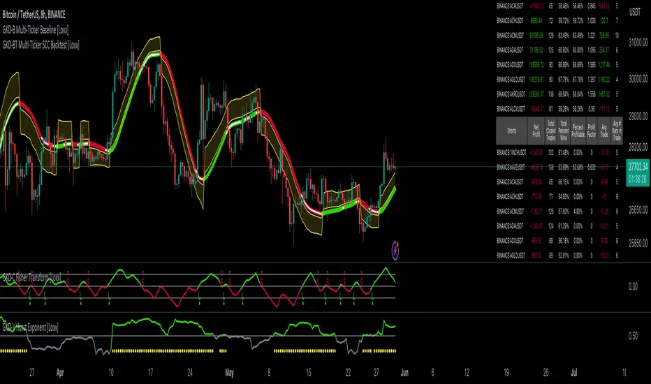
GKD-BT Multi-Ticker SCS Backtest [Loxx]The Giga Kaleidoscope GKD-BT Multi-Ticker SCS Backtest is a backtesting module included in Loxx's "Giga Kaleidoscope Modularized Trading System."
The Multi-Ticker SCS Backtest is a Solo Confirmation Simple backtest that allows traders to test single GKD-C confirmation indicators across 1-10 tickers. The purpose of this backtest is to enable traders to quickly evaluate GKD-C across hundreds of tickers within 30-60 minutes.
The backtest module supports testing with 1 take profit and 1 stop loss. It also offers the option to limit testing to a specific date range, allowing simulated forward testing using historical data. This backtest module only includes standard long and short signals. Additionally, users can choose to display or hide a trading panel that provides relevant information about the backtest, statistics, and the current trade. Traders can also select a highlighting treshold for Total Percent Wins and Percent Profitable, and Profit Factor.
To use this indicator:
1. Select the "Multi-ticker" option in the GKD-C Confirmation indicator.
2. Import 1-10 tickers into the GKD-C Confirmation indicator.
3. Import the same 1-10 indicators into the GKD-BT Multi-Ticker SCS Backtest.
4. Import the value "Input into NEW GKD-BT Multi-ticker Backtest" from the GKD-C Confirmation indicator into the GKD-BT Multi-Ticker SCS Backtest.
5. When importing tickers, ensure that you import the same type of tickers for all 1-10 tickers. For example, test only FX or Cryptocurrency or Stocks. Do not combine different tradable asset types.
6. Make sure that your chart is set to a ticker that corresponds to the tradable asset type. For cryptocurrency testing, set the chart to BTCUSDT. For Forex testing, set the chart to EURUSD.
This backtest includes the following metrics:
1. Net profit: Overall profit or loss achieved.
2. Total Closed Trades: Total number of closed trades, both winning and losing.
3. Total Percent Wins: Total wins, whether long or short, for the selected time interval regardless of commissions and other profit-modifying addons.
4. Percent Profitable: Total wins, whether long or short, that are also profitable, taking commissions into account.
5. Profit Factor: The ratio of gross profits to gross losses, indicating how much money the strategy made for every unit of money it lost.
6. Average Profit per Trade: The average gain or loss per trade, calculated by dividing the net profit by the total number of closed trades.
7. Average Number of Bars in Trade: The average number of bars that elapsed during trades for all closed trades.
Summary of notable settings:
Input Tickers separated by commas: Allows the user to input tickers separated by commas, specifying the symbols or tickers of financial instruments used in the backtest. The tickers should follow the format "EXCHANGE:TICKER" (e.g., "NASDAQ:AAPL, NYSE:MSFT").
Import GKD-C: Imports the "GKD-C" source, which provides signals or data for the backtest.
Initial Capital: Represents the starting account balance for the backtest, denominated in the base currency of the trading account.
Order Size: Determines the quantity of contracts traded in each trade.
Order Type: Specifies the type of order used in the backtest, either "Contracts" or "% Equity."
Commission: Represents the commission per order or transaction cost incurred in each trade.
**the backtest data rendered to the chart above uses $5 commission per trade and 10% equity per trade with $1 million initial capital. Each backtest result for each ticker assumes these same inputs. The results are NOT cumulative, they are separate and isolate per ticker and trading side, long or short**
Volatility Types included
The GKD system utilizes volatility-based take profits and stop losses. Each take profit and stop loss is calculated as a multiple of volatility. You can change the values of the multipliers in the settings as well.
This module includes 17 types of volatility:
Close-to-Close
Parkinson
Garman-Klass
Rogers-Satchell
Yang-Zhang
Garman-Klass-Yang-Zhang
Exponential Weighted Moving Average
Standard Deviation of Log Returns
Pseudo GARCH(2,2)
Average True Range
True Range Double
Standard Deviation
Adaptive Deviation
Median Absolute Deviation
Efficiency-Ratio Adaptive ATR
Mean Absolute Deviation
Static Percent
Various volatility estimators and indicators that investors and traders can use to measure the dispersion or volatility of a financial instrument's price. Each estimator has its strengths and weaknesses, and the choice of estimator should depend on the specific needs and circumstances of the user.
Close-to-Close
Close-to-Close volatility is a classic and widely used volatility measure, sometimes referred to as historical volatility.
Volatility is an indicator of the speed of a stock price change. A stock with high volatility is one where the price changes rapidly and with a larger amplitude. The more volatile a stock is, the riskier it is.
Close-to-close historical volatility is calculated using only a stock's closing prices. It is the simplest volatility estimator. However, in many cases, it is not precise enough. Stock prices could jump significantly during a trading session and return to the opening value at the end. That means that a considerable amount of price information is not taken into account by close-to-close volatility.
Despite its drawbacks, Close-to-Close volatility is still useful in cases where the instrument doesn't have intraday prices. For example, mutual funds calculate their net asset values daily or weekly, and thus their prices are not suitable for more sophisticated volatility estimators.
Parkinson
Parkinson volatility is a volatility measure that uses the stock’s high and low price of the day.
The main difference between regular volatility and Parkinson volatility is that the latter uses high and low prices for a day, rather than only the closing price. This is useful as close-to-close prices could show little difference while large price movements could have occurred during the day. Thus, Parkinson's volatility is considered more precise and requires less data for calculation than close-to-close volatility.
One drawback of this estimator is that it doesn't take into account price movements after the market closes. Hence, it systematically undervalues volatility. This drawback is addressed in the Garman-Klass volatility estimator.
Garman-Klass
Garman-Klass is a volatility estimator that incorporates open, low, high, and close prices of a security.
Garman-Klass volatility extends Parkinson's volatility by taking into account the opening and closing prices. As markets are most active during the opening and closing of a trading session, it makes volatility estimation more accurate.
Garman and Klass also assumed that the process of price change follows a continuous diffusion process (Geometric Brownian motion). However, this assumption has several drawbacks. The method is not robust for opening jumps in price and trend movements.
Despite its drawbacks, the Garman-Klass estimator is still more effective than the basic formula since it takes into account not only the price at the beginning and end of the time interval but also intraday price extremes.
Researchers Rogers and Satchell have proposed a more efficient method for assessing historical volatility that takes into account price trends. See Rogers-Satchell Volatility for more detail.
Rogers-Satchell
Rogers-Satchell is an estimator for measuring the volatility of securities with an average return not equal to zero.
Unlike Parkinson and Garman-Klass estimators, Rogers-Satchell incorporates a drift term (mean return not equal to zero). As a result, it provides better volatility estimation when the underlying is trending.
The main disadvantage of this method is that it does not take into account price movements between trading sessions. This leads to an underestimation of volatility since price jumps periodically occur in the market precisely at the moments between sessions.
A more comprehensive estimator that also considers the gaps between sessions was developed based on the Rogers-Satchel formula in the 2000s by Yang-Zhang. See Yang Zhang Volatility for more detail.
Yang-Zhang
Yang Zhang is a historical volatility estimator that handles both opening jumps and the drift and has a minimum estimation error.
Yang-Zhang volatility can be thought of as a combination of the overnight (close-to-open volatility) and a weighted average of the Rogers-Satchell volatility and the day’s open-to-close volatility. It is considered to be 14 times more efficient than the close-to-close estimator.
Garman-Klass-Yang-Zhang
Garman-Klass-Yang-Zhang (GKYZ) volatility estimator incorporates the returns of open, high, low, and closing prices in its calculation.
GKYZ volatility estimator takes into account overnight jumps but not the trend, i.e., it assumes that the underlying asset follows a Geometric Brownian Motion (GBM) process with zero drift. Therefore, the GKYZ volatility estimator tends to overestimate the volatility when the drift is different from zero. However, for a GBM process, this estimator is eight times more efficient than the close-to-close volatility estimator.
Exponential Weighted Moving Average
The Exponentially Weighted Moving Average (EWMA) is a quantitative or statistical measure used to model or describe a time series. The EWMA is widely used in finance, with the main applications being technical analysis and volatility modeling.
The moving average is designed such that older observations are given lower weights. The weights decrease exponentially as the data point gets older – hence the name exponentially weighted.
The only decision a user of the EWMA must make is the parameter lambda. The parameter decides how important the current observation is in the calculation of the EWMA. The higher the value of lambda, the more closely the EWMA tracks the original time series.
Standard Deviation of Log Returns
This is the simplest calculation of volatility. It's the standard deviation of ln(close/close(1)).
Pseudo GARCH(2,2)
This is calculated using a short- and long-run mean of variance multiplied by ?.
?avg(var;M) + (1 ? ?) avg(var;N) = 2?var/(M+1-(M-1)L) + 2(1-?)var/(M+1-(M-1)L)
Solving for ? can be done by minimizing the mean squared error of estimation; that is, regressing L^-1var - avg(var; N) against avg(var; M) - avg(var; N) and using the resulting beta estimate as ?.
Average True Range
The average true range (ATR) is a technical analysis indicator, introduced by market technician J. Welles Wilder Jr. in his book New Concepts in Technical Trading Systems, that measures market volatility by decomposing the entire range of an asset price for that period.
The true range indicator is taken as the greatest of the following: current high less the current low; the absolute value of the current high less the previous close; and the absolute value of the current low less the previous close. The ATR is then a moving average, generally using 14 days, of the true ranges.
True Range Double
A special case of ATR that attempts to correct for volatility skew.
Standard Deviation
Standard deviation is a statistic that measures the dispersion of a dataset relative to its mean and is calculated as the square root of the variance. The standard deviation is calculated as the square root of variance by determining each data point's deviation relative to the mean. If the data points are further from the mean, there is a higher deviation within the data set; thus, the more spread out the data, the higher the standard deviation.
Adaptive Deviation
By definition, the Standard Deviation (STD, also represented by the Greek letter sigma ? or the Latin letter s) is a measure that is used to quantify the amount of variation or dispersion of a set of data values. In technical analysis, we usually use it to measure the level of current volatility.
Standard Deviation is based on Simple Moving Average calculation for mean value. This version of standard deviation uses the properties of EMA to calculate what can be called a new type of deviation, and since it is based on EMA, we can call it EMA deviation. Additionally, Perry Kaufman's efficiency ratio is used to make it adaptive (since all EMA type calculations are nearly perfect for adapting).
The difference when compared to the standard is significant--not just because of EMA usage, but the efficiency ratio makes it a "bit more logical" in very volatile market conditions.
Median Absolute Deviation
The median absolute deviation is a measure of statistical dispersion. Moreover, the MAD is a robust statistic, being more resilient to outliers in a data set than the standard deviation. In the standard deviation, the distances from the mean are squared, so large deviations are weighted more heavily, and thus outliers can heavily influence it. In the MAD, the deviations of a small number of outliers are irrelevant.
Because the MAD is a more robust estimator of scale than the sample variance or standard deviation, it works better with distributions without a mean or variance, such as the Cauchy distribution.
For this indicator, a manual recreation of the quantile function in Pine Script is used. This is so users have a full inside view into how this is calculated.
Efficiency-Ratio Adaptive ATR
Average True Range (ATR) is a widely used indicator for many occasions in technical analysis. It is calculated as the RMA of the true range. This version adds a "twist": it uses Perry Kaufman's Efficiency Ratio to calculate adaptive true range.
Mean Absolute Deviation
The mean absolute deviation (MAD) is a measure of variability that indicates the average distance between observations and their mean. MAD uses the original units of the data, which simplifies interpretation. Larger values signify that the data points spread out further from the average. Conversely, lower values correspond to data points bunching closer to it. The mean absolute deviation is also known as the mean deviation and average absolute deviation.
This definition of the mean absolute deviation sounds similar to the standard deviation (SD). While both measure variability, they have different calculations. In recent years, some proponents of MAD have suggested that it replace the SD as the primary measure because it is a simpler concept that better fits real life.
█ Giga Kaleidoscope Modularized Trading System
Core components of an NNFX algorithmic trading strategy
The NNFX algorithm is built on the principles of trend, momentum, and volatility. There are six core components in the NNFX trading algorithm:
1. Volatility - price volatility; e.g., Average True Range, True Range Double, Close-to-Close, etc.
2. Baseline - a moving average to identify price trend
3. Confirmation 1 - a technical indicator used to identify trends
4. Confirmation 2 - a technical indicator used to identify trends
5. Continuation - a technical indicator used to identify trends
6. Volatility/Volume - a technical indicator used to identify volatility/volume breakouts/breakdown
7. Exit - a technical indicator used to determine when a trend is exhausted
8. Metamorphosis - a technical indicator that produces a compound signal from the combination of other GKD indicators*
*(not part of the NNFX algorithm)
What is Volatility in the NNFX trading system?
In the NNFX (No Nonsense Forex) trading system, ATR (Average True Range) is typically used to measure the volatility of an asset. It is used as a part of the system to help determine the appropriate stop loss and take profit levels for a trade. ATR is calculated by taking the average of the true range values over a specified period.
True range is calculated as the maximum of the following values:
-Current high minus the current low
-Absolute value of the current high minus the previous close
-Absolute value of the current low minus the previous close
ATR is a dynamic indicator that changes with changes in volatility. As volatility increases, the value of ATR increases, and as volatility decreases, the value of ATR decreases. By using ATR in NNFX system, traders can adjust their stop loss and take profit levels according to the volatility of the asset being traded. This helps to ensure that the trade is given enough room to move, while also minimizing potential losses.
Other types of volatility include True Range Double (TRD), Close-to-Close, and Garman-Klass
What is a Baseline indicator?
The baseline is essentially a moving average, and is used to determine the overall direction of the market.
The baseline in the NNFX system is used to filter out trades that are not in line with the long-term trend of the market. The baseline is plotted on the chart along with other indicators, such as the Moving Average (MA), the Relative Strength Index (RSI), and the Average True Range (ATR).
Trades are only taken when the price is in the same direction as the baseline. For example, if the baseline is sloping upwards, only long trades are taken, and if the baseline is sloping downwards, only short trades are taken. This approach helps to ensure that trades are in line with the overall trend of the market, and reduces the risk of entering trades that are likely to fail.
By using a baseline in the NNFX system, traders can have a clear reference point for determining the overall trend of the market, and can make more informed trading decisions. The baseline helps to filter out noise and false signals, and ensures that trades are taken in the direction of the long-term trend.
What is a Confirmation indicator?
Confirmation indicators are technical indicators that are used to confirm the signals generated by primary indicators. Primary indicators are the core indicators used in the NNFX system, such as the Average True Range (ATR), the Moving Average (MA), and the Relative Strength Index (RSI).
The purpose of the confirmation indicators is to reduce false signals and improve the accuracy of the trading system. They are designed to confirm the signals generated by the primary indicators by providing additional information about the strength and direction of the trend.
Some examples of confirmation indicators that may be used in the NNFX system include the Bollinger Bands, the MACD (Moving Average Convergence Divergence), and the MACD Oscillator. These indicators can provide information about the volatility, momentum, and trend strength of the market, and can be used to confirm the signals generated by the primary indicators.
In the NNFX system, confirmation indicators are used in combination with primary indicators and other filters to create a trading system that is robust and reliable. By using multiple indicators to confirm trading signals, the system aims to reduce the risk of false signals and improve the overall profitability of the trades.
What is a Continuation indicator?
In the NNFX (No Nonsense Forex) trading system, a continuation indicator is a technical indicator that is used to confirm a current trend and predict that the trend is likely to continue in the same direction. A continuation indicator is typically used in conjunction with other indicators in the system, such as a baseline indicator, to provide a comprehensive trading strategy.
What is a Volatility/Volume indicator?
Volume indicators, such as the On Balance Volume (OBV), the Chaikin Money Flow (CMF), or the Volume Price Trend (VPT), are used to measure the amount of buying and selling activity in a market. They are based on the trading volume of the market, and can provide information about the strength of the trend. In the NNFX system, volume indicators are used to confirm trading signals generated by the Moving Average and the Relative Strength Index. Volatility indicators include Average Direction Index, Waddah Attar, and Volatility Ratio. In the NNFX trading system, volatility is a proxy for volume and vice versa.
By using volume indicators as confirmation tools, the NNFX trading system aims to reduce the risk of false signals and improve the overall profitability of trades. These indicators can provide additional information about the market that is not captured by the primary indicators, and can help traders to make more informed trading decisions. In addition, volume indicators can be used to identify potential changes in market trends and to confirm the strength of price movements.
What is an Exit indicator?
The exit indicator is used in conjunction with other indicators in the system, such as the Moving Average (MA), the Relative Strength Index (RSI), and the Average True Range (ATR), to provide a comprehensive trading strategy.
The exit indicator in the NNFX system can be any technical indicator that is deemed effective at identifying optimal exit points. Examples of exit indicators that are commonly used include the Parabolic SAR, the Average Directional Index (ADX), and the Chandelier Exit.
The purpose of the exit indicator is to identify when a trend is likely to reverse or when the market conditions have changed, signaling the need to exit a trade. By using an exit indicator, traders can manage their risk and prevent significant losses.
In the NNFX system, the exit indicator is used in conjunction with a stop loss and a take profit order to maximize profits and minimize losses. The stop loss order is used to limit the amount of loss that can be incurred if the trade goes against the trader, while the take profit order is used to lock in profits when the trade is moving in the trader's favor.
Overall, the use of an exit indicator in the NNFX trading system is an important component of a comprehensive trading strategy. It allows traders to manage their risk effectively and improve the profitability of their trades by exiting at the right time.
What is an Metamorphosis indicator?
The concept of a metamorphosis indicator involves the integration of two or more GKD indicators to generate a compound signal. This is achieved by evaluating the accuracy of each indicator and selecting the signal from the indicator with the highest accuracy. As an illustration, let's consider a scenario where we calculate the accuracy of 10 indicators and choose the signal from the indicator that demonstrates the highest accuracy.
The resulting output from the metamorphosis indicator can then be utilized in a GKD-BT backtest by occupying a slot that aligns with the purpose of the metamorphosis indicator. The slot can be a GKD-B, GKD-C, or GKD-E slot, depending on the specific requirements and objectives of the indicator. This allows for seamless integration and utilization of the compound signal within the GKD-BT framework.
How does Loxx's GKD (Giga Kaleidoscope Modularized Trading System) implement the NNFX algorithm outlined above?
Loxx's GKD v2.0 system has five types of modules (indicators/strategies). These modules are:
1. GKD-BT - Backtesting module (Volatility, Number 1 in the NNFX algorithm)
2. GKD-B - Baseline module (Baseline and Volatility/Volume, Numbers 1 and 2 in the NNFX algorithm)
3. GKD-C - Confirmation 1/2 and Continuation module (Confirmation 1/2 and Continuation, Numbers 3, 4, and 5 in the NNFX algorithm)
4. GKD-V - Volatility/Volume module (Confirmation 1/2, Number 6 in the NNFX algorithm)
5. GKD-E - Exit module (Exit, Number 7 in the NNFX algorithm)
6. GKD-M - Metamorphosis module (Metamorphosis, Number 8 in the NNFX algorithm, but not part of the NNFX algorithm)
(additional module types will added in future releases)
Each module interacts with every module by passing data to A backtest module wherein the various components of the GKD system are combined to create a trading signal.
That is, the Baseline indicator passes its data to Volatility/Volume. The Volatility/Volume indicator passes its values to the Confirmation 1 indicator. The Confirmation 1 indicator passes its values to the Confirmation 2 indicator. The Confirmation 2 indicator passes its values to the Continuation indicator. The Continuation indicator passes its values to the Exit indicator, and finally, the Exit indicator passes its values to the Backtest strategy.
This chaining of indicators requires that each module conform to Loxx's GKD protocol, therefore allowing for the testing of every possible combination of technical indicators that make up the six components of the NNFX algorithm.
What does the application of the GKD trading system look like?
Example trading system:
Backtest: Multi-Ticker SCS Backtest
Baseline: Hull Moving Average
Volatility/Volume: Hurst Exponent
Confirmation 1: Kase Peak Oscillator
Confirmation 2: uf2018
Continuation: Vortex
Exit: Rex Oscillator
Metamorphosis: Baseline Optimizer
Each GKD indicator is denoted with a module identifier of either: GKD-BT, GKD-B, GKD-C, GKD-V, GKD-M, or GKD-E. This allows traders to understand to which module each indicator belongs and where each indicator fits into the GKD system.
█ Giga Kaleidoscope Modularized Trading System Signals
Standard Entry
1. GKD-C Confirmation gives signal
2. Baseline agrees
3. Price inside Goldie Locks Zone Minimum
4. Price inside Goldie Locks Zone Maximum
5. Confirmation 2 agrees
6. Volatility/Volume agrees
1-Candle Standard Entry
1a. GKD-C Confirmation gives signal
2a. Baseline agrees
3a. Price inside Goldie Locks Zone Minimum
4a. Price inside Goldie Locks Zone Maximum
Next Candle
1b. Price retraced
2b. Baseline agrees
3b. Confirmation 1 agrees
4b. Confirmation 2 agrees
5b. Volatility/Volume agrees
Baseline Entry
1. GKD-B Basline gives signal
2. Confirmation 1 agrees
3. Price inside Goldie Locks Zone Minimum
4. Price inside Goldie Locks Zone Maximum
5. Confirmation 2 agrees
6. Volatility/Volume agrees
7. Confirmation 1 signal was less than 'Maximum Allowable PSBC Bars Back' prior
1-Candle Baseline Entry
1a. GKD-B Baseline gives signal
2a. Confirmation 1 agrees
3a. Price inside Goldie Locks Zone Minimum
4a. Price inside Goldie Locks Zone Maximum
5a. Confirmation 1 signal was less than 'Maximum Allowable PSBC Bars Back' prior
Next Candle
1b. Price retraced
2b. Baseline agrees
3b. Confirmation 1 agrees
4b. Confirmation 2 agrees
5b. Volatility/Volume agrees
Volatility/Volume Entry
1. GKD-V Volatility/Volume gives signal
2. Confirmation 1 agrees
3. Price inside Goldie Locks Zone Minimum
4. Price inside Goldie Locks Zone Maximum
5. Confirmation 2 agrees
6. Baseline agrees
7. Confirmation 1 signal was less than 7 candles prior
1-Candle Volatility/Volume Entry
1a. GKD-V Volatility/Volume gives signal
2a. Confirmation 1 agrees
3a. Price inside Goldie Locks Zone Minimum
4a. Price inside Goldie Locks Zone Maximum
5a. Confirmation 1 signal was less than 'Maximum Allowable PSVVC Bars Back' prior
Next Candle
1b. Price retraced
2b. Volatility/Volume agrees
3b. Confirmation 1 agrees
4b. Confirmation 2 agrees
5b. Baseline agrees
Confirmation 2 Entry
1. GKD-C Confirmation 2 gives signal
2. Confirmation 1 agrees
3. Price inside Goldie Locks Zone Minimum
4. Price inside Goldie Locks Zone Maximum
5. Volatility/Volume agrees
6. Baseline agrees
7. Confirmation 1 signal was less than 7 candles prior
1-Candle Confirmation 2 Entry
1a. GKD-C Confirmation 2 gives signal
2a. Confirmation 1 agrees
3a. Price inside Goldie Locks Zone Minimum
4a. Price inside Goldie Locks Zone Maximum
5a. Confirmation 1 signal was less than 'Maximum Allowable PSC2C Bars Back' prior
Next Candle
1b. Price retraced
2b. Confirmation 2 agrees
3b. Confirmation 1 agrees
4b. Volatility/Volume agrees
5b. Baseline agrees
PullBack Entry
1a. GKD-B Baseline gives signal
2a. Confirmation 1 agrees
3a. Price is beyond 1.0x Volatility of Baseline
Next Candle
1b. Price inside Goldie Locks Zone Minimum
2b. Price inside Goldie Locks Zone Maximum
3b. Confirmation 1 agrees
4b. Confirmation 2 agrees
5b. Volatility/Volume agrees
Continuation Entry
1. Standard Entry, 1-Candle Standard Entry, Baseline Entry, 1-Candle Baseline Entry, Volatility/Volume Entry, 1-Candle Volatility/Volume Entry, Confirmation 2 Entry, 1-Candle Confirmation 2 Entry, or Pullback entry triggered previously
2. Baseline hasn't crossed since entry signal trigger
4. Confirmation 1 agrees
5. Baseline agrees
6. Confirmation 2 agrees
█ Connecting to Backtests
All GKD indicators are chained indicators meaning you export the value of the indicators to specialized backtest to creat your GKD trading system. Each indicator contains a proprietary signal generation algo that will only work with GKD backtests. You can find these backtests using the links below.
GKD-BT Giga Confirmation Stack Backtest
GKD-BT Giga Stacks Backtest
GKD-BT Full Giga Kaleidoscope Backtest
GKD-BT Solo Confirmation Super Complex Backtest
GKD-BT Solo Confirmation Complex Backtest
GKD-BT Solo Confirmation Simple Backtest
GKD-M Baseline Optimizer
GKD-M Accuracy Alchemist
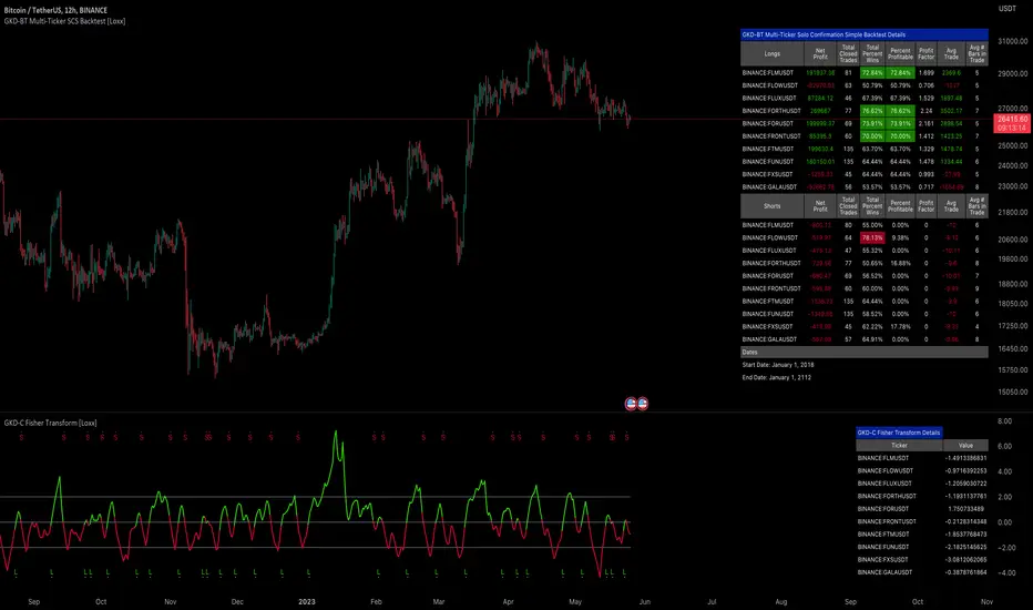
GKD-M Baseline Optimizer [Loxx]Giga Kaleidoscope GKD-M Baseline Optimizer is a Metamorphosis module included in Loxx's "Giga Kaleidoscope Modularized Trading System".
The Baseline Optimizer enables traders to backtest over 60 moving averages using variable period inputs. It then exports the baseline with the highest cumulative win rate per candle to any baseline-enabled GKD backtest. To perform the backtesting, the trader selects an initial period input (default is 60) and a skip value that increments the initial period input up to seven times. For instance, if a skip value of 5 is chosen, the Baseline Optimizer will run the backtest for the selected moving average on periods such as 60, 65, 70, 75, and so on, up to 90. If the user selects an initial period input of 45 and a skip value of 2, the Baseline Optimizer will conduct backtests for the chosen moving average on periods like 45, 47, 49, 51, and so forth, up to 57.
The Baseline Optimizer provides a table displaying the output of the backtests for a specified date range. The table output represents the cumulative win rate for the given date range.
On the Metamorphosis side of the Baseline Optimizer, a cumulative backtest is calculated for each candle within the date range. This means that each candle may exhibit a different distribution of period inputs with the highest win rate for a particular moving average. The Baseline Optimizer identifies the period input combination with the highest win rates for long and short positions and creates a win-rate adaptive long and short moving average chart. The moving average used for shorts differs from the moving average used for longs, and the moving average for each candle may vary from any other candle. This customized baseline can then be exported to all baseline-enabled GKD backtests.
The backtest employed in the Baseline Optimizer is a Solo Confirmation Simple, allowing only one take profit and one stop loss to be set.
Lastly, the Baseline Optimizer incorporates Goldie Locks Zone filtering, which can be utilized for signal generation in advanced GKD backtests.
█ Moving Averages included in the Baseline Optimizer
Adaptive Moving Average - AMA
ADXvma - Average Directional Volatility Moving Average
Ahrens Moving Average
Alexander Moving Average - ALXMA
Deviation Scaled Moving Average - DSMA
Donchian
Double Exponential Moving Average - DEMA
Double Smoothed Exponential Moving Average - DSEMA
Double Smoothed FEMA - DSFEMA
Double Smoothed Range Weighted EMA - DSRWEMA
Double Smoothed Wilders EMA - DSWEMA
Double Weighted Moving Average - DWMA
Exponential Moving Average - EMA
Fast Exponential Moving Average - FEMA
Fractal Adaptive Moving Average - FRAMA
Generalized DEMA - GDEMA
Generalized Double DEMA - GDDEMA
Hull Moving Average (Type 1) - HMA1
Hull Moving Average (Type 2) - HMA2
Hull Moving Average (Type 3) - HMA3
Hull Moving Average (Type 4) - HMA4
IE /2 - Early T3 by Tim Tilson
Integral of Linear Regression Slope - ILRS
Kaufman Adaptive Moving Average - KAMA
Leader Exponential Moving Average
Linear Regression Value - LSMA ( Least Squares Moving Average )
Linear Weighted Moving Average - LWMA
McGinley Dynamic
McNicholl EMA
Non-Lag Moving Average
Ocean NMA Moving Average - ONMAMA
One More Moving Average - OMA
Parabolic Weighted Moving Average
Probability Density Function Moving Average - PDFMA
Quadratic Regression Moving Average - QRMA
Regularized EMA - REMA
Range Weighted EMA - RWEMA
Recursive Moving Trendline
Simple Decycler - SDEC
Simple Jurik Moving Average - SJMA
Simple Moving Average - SMA
Sine Weighted Moving Average
Smoothed LWMA - SLWMA
Smoothed Moving Average - SMMA
Smoother
Super Smoother
T3
Three-pole Ehlers Butterworth
Three-pole Ehlers Smoother
Triangular Moving Average - TMA
Triple Exponential Moving Average - TEMA
Two-pole Ehlers Butterworth
Two-pole Ehlers smoother
Variable Index Dynamic Average - VIDYA
Variable Moving Average - VMA
Volume Weighted EMA - VEMA
Volume Weighted Moving Average - VWMA
Zero-Lag DEMA - Zero Lag Exponential Moving Average
Zero-Lag Moving Average
Zero Lag TEMA - Zero Lag Triple Exponential Moving Average
Adaptive Moving Average - AMA
The Adaptive Moving Average (AMA) is a moving average that changes its sensitivity to price moves depending on the calculated volatility. It becomes more sensitive during periods when the price is moving smoothly in a certain direction and becomes less sensitive when the price is volatile.
ADXvma - Average Directional Volatility Moving Average
Linnsoft's ADXvma formula is a volatility-based moving average, with the volatility being determined by the value of the ADX indicator.
The ADXvma has the SMA in Chande's CMO replaced with an EMA , it then uses a few more layers of EMA smoothing before the "Volatility Index" is calculated.
A side effect is, those additional layers slow down the ADXvma when you compare it to Chande's Variable Index Dynamic Average VIDYA .
The ADXVMA provides support during uptrends and resistance during downtrends and will stay flat for longer, but will create some of the most accurate market signals when it decides to move.
Ahrens Moving Average
Richard D. Ahrens's Moving Average promises "Smoother Data" that isn't influenced by the occasional price spike. It works by using the Open and the Close in his formula so that the only time the Ahrens Moving Average will change is when the candlestick is either making new highs or new lows.
Alexander Moving Average - ALXMA
This Moving Average uses an elaborate smoothing formula and utilizes a 7 period Moving Average. It corresponds to fitting a second-order polynomial to seven consecutive observations. This moving average is rarely used in trading but is interesting as this Moving Average has been applied to diffusion indexes that tend to be very volatile.
Deviation Scaled Moving Average - DSMA
The Deviation-Scaled Moving Average is a data smoothing technique that acts like an exponential moving average with a dynamic smoothing coefficient. The smoothing coefficient is automatically updated based on the magnitude of price changes. In the Deviation-Scaled Moving Average, the standard deviation from the mean is chosen to be the measure of this magnitude. The resulting indicator provides substantial smoothing of the data even when price changes are small while quickly adapting to these changes.
Donchian
Donchian Channels are three lines generated by moving average calculations that comprise an indicator formed by upper and lower bands around a midrange or median band. The upper band marks the highest price of a security over N periods while the lower band marks the lowest price of a security over N periods.
Double Exponential Moving Average - DEMA
The Double Exponential Moving Average ( DEMA ) combines a smoothed EMA and a single EMA to provide a low-lag indicator. It's primary purpose is to reduce the amount of "lagging entry" opportunities, and like all Moving Averages, the DEMA confirms uptrends whenever price crosses on top of it and closes above it, and confirms downtrends when the price crosses under it and closes below it - but with significantly less lag.
Double Smoothed Exponential Moving Average - DSEMA
The Double Smoothed Exponential Moving Average is a lot less laggy compared to a traditional EMA . It's also considered a leading indicator compared to the EMA , and is best utilized whenever smoothness and speed of reaction to market changes are required.
Double Smoothed FEMA - DSFEMA
Same as the Double Exponential Moving Average (DEMA), but uses a faster version of EMA for its calculation.
Double Smoothed Range Weighted EMA - DSRWEMA
Range weighted exponential moving average (EMA) is, unlike the "regular" range weighted average calculated in a different way. Even though the basis - the range weighting - is the same, the way how it is calculated is completely different. By definition this type of EMA is calculated as a ratio of EMA of price*weight / EMA of weight. And the results are very different and the two should be considered as completely different types of averages. The higher than EMA to price changes responsiveness when the ranges increase remains in this EMA too and in those cases this EMA is clearly leading the "regular" EMA. This version includes double smoothing.
Double Smoothed Wilders EMA - DSWEMA
Welles Wilder was frequently using one "special" case of EMA (Exponential Moving Average) that is due to that fact (that he used it) sometimes called Wilder's EMA. This version is adding double smoothing to Wilder's EMA in order to make it "faster" (it is more responsive to market prices than the original) and is still keeping very smooth values.
Double Weighted Moving Average - DWMA
Double weighted moving average is an LWMA (Linear Weighted Moving Average). Instead of doing one cycle for calculating the LWMA, the indicator is made to cycle the loop 2 times. That produces a smoother values than the original LWMA
Exponential Moving Average - EMA
The EMA places more significance on recent data points and moves closer to price than the SMA ( Simple Moving Average ). It reacts faster to volatility due to its emphasis on recent data and is known for its ability to give greater weight to recent and more relevant data. The EMA is therefore seen as an enhancement over the SMA .
Fast Exponential Moving Average - FEMA
An Exponential Moving Average with a short look-back period.
Fractal Adaptive Moving Average - FRAMA
The Fractal Adaptive Moving Average by John Ehlers is an intelligent adaptive Moving Average which takes the importance of price changes into account and follows price closely enough to display significant moves whilst remaining flat if price ranges. The FRAMA does this by dynamically adjusting the look-back period based on the market's fractal geometry.
Generalized DEMA - GDEMA
The double exponential moving average (DEMA), was developed by Patrick Mulloy in an attempt to reduce the amount of lag time found in traditional moving averages. It was first introduced in the February 1994 issue of the magazine Technical Analysis of Stocks & Commodities in Mulloy's article "Smoothing Data with Faster Moving Averages.". Instead of using fixed multiplication factor in the final DEMA formula, the generalized version allows you to change it. By varying the "volume factor" form 0 to 1 you apply different multiplications and thus producing DEMA with different "speed" - the higher the volume factor is the "faster" the DEMA will be (but also the slope of it will be less smooth). The volume factor is limited in the calculation to 1 since any volume factor that is larger than 1 is increasing the overshooting to the extent that some volume factors usage makes the indicator unusable.
Generalized Double DEMA - GDDEMA
The double exponential moving average (DEMA), was developed by Patrick Mulloy in an attempt to reduce the amount of lag time found in traditional moving averages. It was first introduced in the February 1994 issue of the magazine Technical Analysis of Stocks & Commodities in Mulloy's article "Smoothing Data with Faster Moving Averages''. This is an extension of the Generalized DEMA using Tim Tillsons (the inventor of T3) idea, and is using GDEMA of GDEMA for calculation (which is the "middle step" of T3 calculation). Since there are no versions showing that middle step, this version covers that too. The result is smoother than Generalized DEMA, but is less smooth than T3 - one has to do some experimenting in order to find the optimal way to use it, but in any case, since it is "faster" than the T3 (Tim Tillson T3) and still smooth, it looks like a good compromise between speed and smoothness.
Hull Moving Average (Type 1) - HMA1
Alan Hull's HMA makes use of weighted moving averages to prioritize recent values and greatly reduce lag whilst maintaining the smoothness of a traditional Moving Average. For this reason, it's seen as a well-suited Moving Average for identifying entry points. This version uses SMA for smoothing.
Hull Moving Average (Type 2) - HMA2
Alan Hull's HMA makes use of weighted moving averages to prioritize recent values and greatly reduce lag whilst maintaining the smoothness of a traditional Moving Average. For this reason, it's seen as a well-suited Moving Average for identifying entry points. This version uses EMA for smoothing.
Hull Moving Average (Type 3) - HMA3
Alan Hull's HMA makes use of weighted moving averages to prioritize recent values and greatly reduce lag whilst maintaining the smoothness of a traditional Moving Average. For this reason, it's seen as a well-suited Moving Average for identifying entry points. This version uses LWMA for smoothing.
Hull Moving Average (Type 4) - HMA4
Alan Hull's HMA makes use of weighted moving averages to prioritize recent values and greatly reduce lag whilst maintaining the smoothness of a traditional Moving Average. For this reason, it's seen as a well-suited Moving Average for identifying entry points. This version uses SMMA for smoothing.
IE /2 - Early T3 by Tim Tilson and T3 new
The T3 moving average is a type of technical indicator used in financial analysis to identify trends in price movements. It is similar to the Exponential Moving Average (EMA) and the Double Exponential Moving Average (DEMA), but uses a different smoothing algorithm.
The T3 moving average is calculated using a series of exponential moving averages that are designed to filter out noise and smooth the data. The resulting smoothed data is then weighted with a non-linear function to produce a final output that is more responsive to changes in trend direction.
The T3 moving average can be customized by adjusting the length of the moving average, as well as the weighting function used to smooth the data. It is commonly used in conjunction with other technical indicators as part of a larger trading strategy.
Integral of Linear Regression Slope - ILRS
A Moving Average where the slope of a linear regression line is simply integrated as it is fitted in a moving window of length N (natural numbers in maths) across the data. The derivative of ILRS is the linear regression slope. ILRS is not the same as a SMA ( Simple Moving Average ) of length N, which is actually the midpoint of the linear regression line as it moves across the data.
Kaufman Adaptive Moving Average - KAMA
Developed by Perry Kaufman, Kaufman's Adaptive Moving Average (KAMA) is a moving average designed to account for market noise or volatility. KAMA will closely follow prices when the price swings are relatively small and the noise is low.
Leader Exponential Moving Average
The Leader EMA was created by Giorgos E. Siligardos who created a Moving Average which was able to eliminate lag altogether whilst maintaining some smoothness. It was first described during his research paper "MACD Leader" where he applied this to the MACD to improve its signals and remove its lagging issue. This filter uses his leading MACD's "modified EMA" and can be used as a zero lag filter.
Linear Regression Value - LSMA ( Least Squares Moving Average )
LSMA as a Moving Average is based on plotting the end point of the linear regression line. It compares the current value to the prior value and a determination is made of a possible trend, eg. the linear regression line is pointing up or down.
Linear Weighted Moving Average - LWMA
LWMA reacts to price quicker than the SMA and EMA . Although it's similar to the Simple Moving Average , the difference is that a weight coefficient is multiplied to the price which means the most recent price has the highest weighting, and each prior price has progressively less weight. The weights drop in a linear fashion.
McGinley Dynamic
John McGinley created this Moving Average to track prices better than traditional Moving Averages. It does this by incorporating an automatic adjustment factor into its formula, which speeds (or slows) the indicator in trending, or ranging, markets.
McNicholl EMA
Dennis McNicholl developed this Moving Average to use as his center line for his "Better Bollinger Bands" indicator and was successful because it responded better to volatility changes over the standard SMA and managed to avoid common whipsaws.
Non-lag moving average
The Non Lag Moving average follows price closely and gives very quick signals as well as early signals of price change. As a standalone Moving Average, it should not be used on its own, but as an additional confluence tool for early signals.
Ocean NMA Moving Average - ONMAMA
Created by Jim Sloman, the NMA is a moving average that automatically adjusts to volatility without being programmed to do so. For more info, read his guide "Ocean Theory, an Introduction"
One More Moving Average (OMA)
The One More Moving Average (OMA) is a technical indicator that calculates a series of Jurik-style moving averages in order to reduce noise and provide smoother price data. It uses six exponential moving averages to generate the final value, with the length of the moving averages determined by an adaptive algorithm that adjusts to the current market conditions. The algorithm calculates the average period by comparing the signal to noise ratio and using this value to determine the length of the moving averages. The resulting values are used to generate the final value of the OMA, which can be used to identify trends and potential changes in trend direction.
Parabolic Weighted Moving Average
The Parabolic Weighted Moving Average is a variation of the Linear Weighted Moving Average . The Linear Weighted Moving Average calculates the average by assigning different weights to each element in its calculation. The Parabolic Weighted Moving Average is a variation that allows weights to be changed to form a parabolic curve. It is done simply by using the Power parameter of this indicator.
Probability Density Function Moving Average - PDFMA
Probability density function based MA is a sort of weighted moving average that uses probability density function to calculate the weights. By its nature it is similar to a lot of digital filters.
Quadratic Regression Moving Average - QRMA
A quadratic regression is the process of finding the equation of the parabola that best fits a set of data. This moving average is an obscure concept that was posted to Forex forums in around 2008.
Regularized EMA - REMA
The regularized exponential moving average (REMA) by Chris Satchwell is a variation on the EMA (see Exponential Moving Average) designed to be smoother but not introduce too much extra lag.
Range Weighted EMA - RWEMA
This indicator is a variation of the range weighted EMA. The variation comes from a possible need to make that indicator a bit less "noisy" when it comes to slope changes. The method used for calculating this variation is the method described by Lee Leibfarth in his article "Trading With An Adaptive Price Zone".
Recursive Moving Trendline
Dennis Meyers's Recursive Moving Trendline uses a recursive (repeated application of a rule) polynomial fit, a technique that uses a small number of past values estimations of price and today's price to predict tomorrow's price.
Simple Decycler - SDEC
The Ehlers Simple Decycler study is a virtually zero-lag technical indicator proposed by John F. Ehlers. The original idea behind this study (and several others created by John F. Ehlers) is that market data can be considered a continuum of cycle periods with different cycle amplitudes. Thus, trending periods can be considered segments of longer cycles, or, in other words, low-frequency segments. Applying the right filter might help identify these segments.
Simple Loxx Moving Average - SLMA
A three stage moving average combining an adaptive EMA, a Kalman Filter, and a Kauffman adaptive filter.
Simple Moving Average - SMA
The SMA calculates the average of a range of prices by adding recent prices and then dividing that figure by the number of time periods in the calculation average. It is the most basic Moving Average which is seen as a reliable tool for starting off with Moving Average studies. As reliable as it may be, the basic moving average will work better when it's enhanced into an EMA .
Sine Weighted Moving Average
The Sine Weighted Moving Average assigns the most weight at the middle of the data set. It does this by weighting from the first half of a Sine Wave Cycle and the most weighting is given to the data in the middle of that data set. The Sine WMA closely resembles the TMA (Triangular Moving Average).
Smoothed LWMA - SLWMA
A smoothed version of the LWMA
Smoothed Moving Average - SMMA
The Smoothed Moving Average is similar to the Simple Moving Average ( SMA ), but aims to reduce noise rather than reduce lag. SMMA takes all prices into account and uses a long lookback period. Due to this, it's seen as an accurate yet laggy Moving Average.
Smoother
The Smoother filter is a faster-reacting smoothing technique which generates considerably less lag than the SMMA ( Smoothed Moving Average ). It gives earlier signals but can also create false signals due to its earlier reactions. This filter is sometimes wrongly mistaken for the superior Jurik Smoothing algorithm.
Super Smoother
The Super Smoother filter uses John Ehlers’s “Super Smoother” which consists of a Two pole Butterworth filter combined with a 2-bar SMA ( Simple Moving Average ) that suppresses the 22050 Hz Nyquist frequency: A characteristic of a sampler, which converts a continuous function or signal into a discrete sequence.
Three-pole Ehlers Butterworth
The 3 pole Ehlers Butterworth (as well as the Two pole Butterworth) are both superior alternatives to the EMA and SMA . They aim at producing less lag whilst maintaining accuracy. The 2 pole filter will give you a better approximation for price, whereas the 3 pole filter has superior smoothing.
Three-pole Ehlers smoother
The 3 pole Ehlers smoother works almost as close to price as the above mentioned 3 Pole Ehlers Butterworth. It acts as a strong baseline for signals but removes some noise. Side by side, it hardly differs from the Three Pole Ehlers Butterworth but when examined closely, it has better overshoot reduction compared to the 3 pole Ehlers Butterworth.
Triangular Moving Average - TMA
The TMA is similar to the EMA but uses a different weighting scheme. Exponential and weighted Moving Averages will assign weight to the most recent price data. Simple moving averages will assign the weight equally across all the price data. With a TMA (Triangular Moving Average), it is double smoother (averaged twice) so the majority of the weight is assigned to the middle portion of the data.
Triple Exponential Moving Average - TEMA
The TEMA uses multiple EMA calculations as well as subtracting lag to create a tool which can be used for scalping pullbacks. As it follows price closely, its signals are considered very noisy and should only be used in extremely fast-paced trading conditions.
Two-pole Ehlers Butterworth
The 2 pole Ehlers Butterworth (as well as the three pole Butterworth mentioned above) is another filter that cuts out the noise and follows the price closely. The 2 pole is seen as a faster, leading filter over the 3 pole and follows price a bit more closely. Analysts will utilize both a 2 pole and a 3 pole Butterworth on the same chart using the same period, but having both on chart allows its crosses to be traded.
Two-pole Ehlers smoother
A smoother version of the Two pole Ehlers Butterworth. This filter is the faster version out of the 3 pole Ehlers Butterworth. It does a decent job at cutting out market noise whilst emphasizing a closer following to price over the 3 pole Ehlers .
Variable Index Dynamic Average - VIDYA
Variable Index Dynamic Average Technical Indicator ( VIDYA ) was developed by Tushar Chande. It is an original method of calculating the Exponential Moving Average ( EMA ) with the dynamically changing period of averaging.
Variable Moving Average - VMA
The Variable Moving Average (VMA) is a study that uses an Exponential Moving Average being able to automatically adjust its smoothing factor according to the market volatility.
Volume Weighted EMA - VEMA
An EMA that uses a volume and price weighted calculation instead of the standard price input.
Volume Weighted Moving Average - VWMA
A Volume Weighted Moving Average is a moving average where more weight is given to bars with heavy volume than with light volume. Thus the value of the moving average will be closer to where most trading actually happened than it otherwise would be without being volume weighted.
Zero-Lag DEMA - Zero Lag Double Exponential Moving Average
John Ehlers's Zero Lag DEMA's aim is to eliminate the inherent lag associated with all trend following indicators which average a price over time. Because this is a Double Exponential Moving Average with Zero Lag, it has a tendency to overshoot and create a lot of false signals for swing trading. It can however be used for quick scalping or as a secondary indicator for confluence.
Zero-Lag Moving Average
The Zero Lag Moving Average is described by its creator, John Ehlers , as a Moving Average with absolutely no delay. And it's for this reason that this filter will cause a lot of abrupt signals which will not be ideal for medium to long-term traders. This filter is designed to follow price as close as possible whilst de-lagging data instead of basing it on regular data. The way this is done is by attempting to remove the cumulative effect of the Moving Average.
Zero-Lag TEMA - Zero Lag Triple Exponential Moving Average
Just like the Zero Lag DEMA , this filter will give you the fastest signals out of all the Zero Lag Moving Averages. This is useful for scalping but dangerous for medium to long-term traders, especially during market Volatility and news events. Having no lag, this filter also has no smoothing in its signals and can cause some very bizarre behavior when applied to certain indicators.
█ Volatility Goldie Locks Zone
The Goldie Locks Zone volatility filter is the standard first-pass filter used in all advanced GKD backtests (Complex, Super Complex, and Full GKd). This filter requires the price to fall within a range determined by multiples of volatility. The Goldie Locks Zone is separate from the core Baseline and utilizes its own moving average with Loxx's Exotic Source Types you can read about below.
On the chart, you will find green and red dots positioned at the top, indicating whether a candle qualifies for a long or short trade respectively. Additionally, green and red triangles are located at the bottom of the chart, signifying whether the trigger has crossed up or down and qualifies within the Goldie Locks zone. The Goldie Locks zone is represented by a white color on the mean line, indicating low volatility levels that are not suitable for trading.
█ Volatility Types Included in the Baseline Optimizer
The GKD system utilizes volatility-based take profits and stop losses. Each take profit and stop loss is calculated as a multiple of volatility. Users can also adjust the multiplier values in the settings.
This module includes 17 types of volatility:
Close-to-Close
Parkinson
Garman-Klass
Rogers-Satchell
Yang-Zhang
Garman-Klass-Yang-Zhang
Exponential Weighted Moving Average
Standard Deviation of Log Returns
Pseudo GARCH(2,2)
Average True Range
True Range Double
Standard Deviation
Adaptive Deviation
Median Absolute Deviation
Efficiency-Ratio Adaptive ATR
Mean Absolute Deviation
Static Percent
Various volatility estimators and indicators that investors and traders can use to measure the dispersion or volatility of a financial instrument's price. Each estimator has its strengths and weaknesses, and the choice of estimator should depend on the specific needs and circumstances of the user.
Close-to-Close
Close-to-Close volatility is a classic and widely used volatility measure, sometimes referred to as historical volatility.
Volatility is an indicator of the speed of a stock price change. A stock with high volatility is one where the price changes rapidly and with a larger amplitude. The more volatile a stock is, the riskier it is.
Close-to-close historical volatility is calculated using only a stock's closing prices. It is the simplest volatility estimator. However, in many cases, it is not precise enough. Stock prices could jump significantly during a trading session and return to the opening value at the end. That means that a considerable amount of price information is not taken into account by close-to-close volatility.
Despite its drawbacks, Close-to-Close volatility is still useful in cases where the instrument doesn't have intraday prices. For example, mutual funds calculate their net asset values daily or weekly, and thus their prices are not suitable for more sophisticated volatility estimators.
Parkinson
Parkinson volatility is a volatility measure that uses the stock’s high and low price of the day.
The main difference between regular volatility and Parkinson volatility is that the latter uses high and low prices for a day, rather than only the closing price. This is useful as close-to-close prices could show little difference while large price movements could have occurred during the day. Thus, Parkinson's volatility is considered more precise and requires less data for calculation than close-to-close volatility.
One drawback of this estimator is that it doesn't take into account price movements after the market closes. Hence, it systematically undervalues volatility. This drawback is addressed in the Garman-Klass volatility estimator.
Garman-Klass
Garman-Klass is a volatility estimator that incorporates open, low, high, and close prices of a security.
Garman-Klass volatility extends Parkinson's volatility by taking into account the opening and closing prices. As markets are most active during the opening and closing of a trading session, it makes volatility estimation more accurate.
Garman and Klass also assumed that the process of price change follows a continuous diffusion process (Geometric Brownian motion). However, this assumption has several drawbacks. The method is not robust for opening jumps in price and trend movements.
Despite its drawbacks, the Garman-Klass estimator is still more effective than the basic formula since it takes into account not only the price at the beginning and end of the time interval but also intraday price extremes.
Researchers Rogers and Satchell have proposed a more efficient method for assessing historical volatility that takes into account price trends. See Rogers-Satchell Volatility for more detail.
Rogers-Satchell
Rogers-Satchell is an estimator for measuring the volatility of securities with an average return not equal to zero.
Unlike Parkinson and Garman-Klass estimators, Rogers-Satchell incorporates a drift term (mean return not equal to zero). As a result, it provides better volatility estimation when the underlying is trending.
The main disadvantage of this method is that it does not take into account price movements between trading sessions. This leads to an underestimation of volatility since price jumps periodically occur in the market precisely at the moments between sessions.
A more comprehensive estimator that also considers the gaps between sessions was developed based on the Rogers-Satchel formula in the 2000s by Yang-Zhang. See Yang Zhang Volatility for more detail.
Yang-Zhang
Yang Zhang is a historical volatility estimator that handles both opening jumps and the drift and has a minimum estimation error.
Yang-Zhang volatility can be thought of as a combination of the overnight (close-to-open volatility) and a weighted average of the Rogers-Satchell volatility and the day’s open-to-close volatility. It is considered to be 14 times more efficient than the close-to-close estimator.
Garman-Klass-Yang-Zhang
Garman-Klass-Yang-Zhang (GKYZ) volatility estimator incorporates the returns of open, high, low, and closing prices in its calculation.
GKYZ volatility estimator takes into account overnight jumps but not the trend, i.e., it assumes that the underlying asset follows a Geometric Brownian Motion (GBM) process with zero drift. Therefore, the GKYZ volatility estimator tends to overestimate the volatility when the drift is different from zero. However, for a GBM process, this estimator is eight times more efficient than the close-to-close volatility estimator.
Exponential Weighted Moving Average
The Exponentially Weighted Moving Average (EWMA) is a quantitative or statistical measure used to model or describe a time series. The EWMA is widely used in finance, with the main applications being technical analysis and volatility modeling.
The moving average is designed such that older observations are given lower weights. The weights decrease exponentially as the data point gets older – hence the name exponentially weighted.
The only decision a user of the EWMA must make is the parameter lambda. The parameter decides how important the current observation is in the calculation of the EWMA. The higher the value of lambda, the more closely the EWMA tracks the original time series.
Standard Deviation of Log Returns
This is the simplest calculation of volatility. It's the standard deviation of ln(close/close(1)).
Pseudo GARCH(2,2)
This is calculated using a short- and long-run mean of variance multiplied by ?.
?avg(var;M) + (1 ? ?) avg(var;N) = 2?var/(M+1-(M-1)L) + 2(1-?)var/(M+1-(M-1)L)
Solving for ? can be done by minimizing the mean squared error of estimation; that is, regressing L^-1var - avg(var; N) against avg(var; M) - avg(var; N) and using the resulting beta estimate as ?.
Average True Range
The average true range (ATR) is a technical analysis indicator, introduced by market technician J. Welles Wilder Jr. in his book New Concepts in Technical Trading Systems, that measures market volatility by decomposing the entire range of an asset price for that period.
The true range indicator is taken as the greatest of the following: current high less the current low; the absolute value of the current high less the previous close; and the absolute value of the current low less the previous close. The ATR is then a moving average, generally using 14 days, of the true ranges.
True Range Double
A special case of ATR that attempts to correct for volatility skew.
Standard Deviation
Standard deviation is a statistic that measures the dispersion of a dataset relative to its mean and is calculated as the square root of the variance. The standard deviation is calculated as the square root of variance by determining each data point's deviation relative to the mean. If the data points are further from the mean, there is a higher deviation within the data set; thus, the more spread out the data, the higher the standard deviation.
Adaptive Deviation
By definition, the Standard Deviation (STD, also represented by the Greek letter sigma ? or the Latin letter s) is a measure that is used to quantify the amount of variation or dispersion of a set of data values. In technical analysis, we usually use it to measure the level of current volatility.
Standard Deviation is based on Simple Moving Average calculation for mean value. This version of standard deviation uses the properties of EMA to calculate what can be called a new type of deviation, and since it is based on EMA, we can call it EMA deviation. Additionally, Perry Kaufman's efficiency ratio is used to make it adaptive (since all EMA type calculations are nearly perfect for adapting).
The difference when compared to the standard is significant--not just because of EMA usage, but the efficiency ratio makes it a "bit more logical" in very volatile market conditions.
Median Absolute Deviation
The median absolute deviation is a measure of statistical dispersion. Moreover, the MAD is a robust statistic, being more resilient to outliers in a data set than the standard deviation. In the standard deviation, the distances from the mean are squared, so large deviations are weighted more heavily, and thus outliers can heavily influence it. In the MAD, the deviations of a small number of outliers are irrelevant.
Because the MAD is a more robust estimator of scale than the sample variance or standard deviation, it works better with distributions without a mean or variance, such as the Cauchy distribution.
For this indicator, a manual recreation of the quantile function in Pine Script is used. This is so users have a full inside view into how this is calculated.
Efficiency-Ratio Adaptive ATR
Average True Range (ATR) is a widely used indicator for many occasions in technical analysis. It is calculated as the RMA of the true range. This version adds a "twist": it uses Perry Kaufman's Efficiency Ratio to calculate adaptive true range.
Mean Absolute Deviation
The mean absolute deviation (MAD) is a measure of variability that indicates the average distance between observations and their mean. MAD uses the original units of the data, which simplifies interpretation. Larger values signify that the data points spread out further from the average. Conversely, lower values correspond to data points bunching closer to it. The mean absolute deviation is also known as the mean deviation and average absolute deviation.
This definition of the mean absolute deviation sounds similar to the standard deviation (SD). While both measure variability, they have different calculations. In recent years, some proponents of MAD have suggested that it replace the SD as the primary measure because it is a simpler concept that better fits real life.
█ Loxx's Expanded Source Types Included in Baseline Optimizer
This indicator allows you to select from 33 source types. They are as follows:
Close
Open
High
Low
Median
Typical
Weighted
Average
Average Median Body
Trend Biased
Trend Biased (Extreme)
HA Close
HA Open
HA High
HA Low
HA Median
HA Typical
HA Weighted
HA Average
HA Average Median Body
HA Trend Biased
HA Trend Biased (Extreme)
HAB Close
HAB Open
HAB High
HAB Low
HAB Median
HAB Typical
HAB Weighted
HAB Average
HAB Average Median Body
HAB Trend Biased
HAB Trend Biased (Extreme)
What are Heiken Ashi "better" candles?
Heiken Ashi "better" candles are a modified version of the standard Heiken Ashi candles, which are a popular charting technique used in technical analysis. Heiken Ashi candles help traders identify trends and potential reversal points by smoothing out price data and reducing market noise. The "better formula" was proposed by Sebastian Schmidt in an article published by BNP Paribas in Warrants & Zertifikate, a German magazine, in August 2004. The aim of this formula is to further improve the smoothing of the Heiken Ashi chart and enhance its effectiveness in identifying trends and reversals.
Standard Heiken Ashi candles are calculated using the following formulas:
Heiken Ashi Close = (Open + High + Low + Close) / 4
Heiken Ashi Open = (Previous Heiken Ashi Open + Previous Heiken Ashi Close) / 2
Heiken Ashi High = Max (High, Heiken Ashi Open, Heiken Ashi Close)
Heiken Ashi Low = Min (Low, Heiken Ashi Open, Heiken Ashi Close)
The "better formula" modifies the standard Heiken Ashi calculation by incorporating additional smoothing, which can help reduce noise and make it easier to identify trends and reversals. The modified formulas for Heiken Ashi "better" candles are as follows:
Better Heiken Ashi Close = (Open + High + Low + Close) / 4
Better Heiken Ashi Open = (Previous Better Heiken Ashi Open + Previous Better Heiken Ashi Close) / 2
Better Heiken Ashi High = Max (High, Better Heiken Ashi Open, Better Heiken Ashi Close)
Better Heiken Ashi Low = Min (Low, Better Heiken Ashi Open, Better Heiken Ashi Close)
Smoothing Factor = 2 / (N + 1), where N is the chosen period for smoothing
Smoothed Better Heiken Ashi Open = (Better Heiken Ashi Open * Smoothing Factor) + (Previous Smoothed Better Heiken Ashi Open * (1 - Smoothing Factor))
Smoothed Better Heiken Ashi Close = (Better Heiken Ashi Close * Smoothing Factor) + (Previous Smoothed Better Heiken Ashi Close * (1 - Smoothing Factor))
The smoothed Better Heiken Ashi Open and Close values are then used to calculate the smoothed Better Heiken Ashi High and Low values, resulting in "better" candles that provide a clearer representation of the market trend and potential reversal points.
Heiken Ashi "better" candles, as mentioned previously, provide a clearer representation of market trends and potential reversal points by reducing noise and smoothing out price data. When using these candles in conjunction with other technical analysis tools and indicators, traders can gain valuable insights into market behavior and make more informed decisions.
To effectively use Heiken Ashi "better" candles in your trading strategy, consider the following tips:
-Trend Identification: Heiken Ashi "better" candles can help you identify the prevailing trend in the market. When the majority of the candles are green (or another color, depending on your chart settings) and there are no or few lower wicks, it may indicate a strong uptrend. Conversely, when the majority of the candles are red (or another color) and there are no or few upper wicks, it may signal a strong downtrend.
-Trend Reversals: Look for potential trend reversals when a change in the color of the candles occurs, especially when accompanied by longer wicks. For example, if a green candle with a long lower wick is followed by a red candle, it could indicate a bearish reversal. Similarly, a red candle with a long upper wick followed by a green candle may suggest a bullish reversal.
-Support and Resistance: You can use Heiken Ashi "better" candles to identify potential support and resistance levels. When the candles are consistently moving in one direction and then suddenly change color with longer wicks, it could indicate the presence of a support or resistance level.
-Stop-Loss and Take-Profit: Using Heiken Ashi "better" candles can help you manage risk by determining optimal stop-loss and take-profit levels. For instance, you can place your stop-loss below the low of the most recent green candle in an uptrend or above the high of the most recent red candle in a downtrend.
-Confirming Signals: Heiken Ashi "better" candles should be used in conjunction with other technical indicators, such as moving averages, oscillators, or chart patterns, to confirm signals and improve the accuracy of your analysis.
In this implementation, you have the choice of AMA, KAMA, or T3 smoothing. These are as follows:
Kaufman Adaptive Moving Average (KAMA)
The Kaufman Adaptive Moving Average (KAMA) is a type of adaptive moving average used in technical analysis to smooth out price fluctuations and identify trends. The KAMA adjusts its smoothing factor based on the market's volatility, making it more responsive in volatile markets and smoother in calm markets. The KAMA is calculated using three different efficiency ratios that determine the appropriate smoothing factor for the current market conditions. These ratios are based on the noise level of the market, the speed at which the market is moving, and the length of the moving average. The KAMA is a popular choice among traders who prefer to use adaptive indicators to identify trends and potential reversals.
Adaptive Moving Average
The Adaptive Moving Average (AMA) is a type of moving average that adjusts its sensitivity to price movements based on market conditions. It uses a ratio between the current price and the highest and lowest prices over a certain lookback period to determine its level of smoothing. The AMA can help reduce lag and increase responsiveness to changes in trend direction, making it useful for traders who want to follow trends while avoiding false signals. The AMA is calculated by multiplying a smoothing constant with the difference between the current price and the previous AMA value, then adding the result to the previous AMA value.
T3
The T3 moving average is a type of technical indicator used in financial analysis to identify trends in price movements. It is similar to the Exponential Moving Average (EMA) and the Double Exponential Moving Average (DEMA), but uses a different smoothing algorithm.
The T3 moving average is calculated using a series of exponential moving averages that are designed to filter out noise and smooth the data. The resulting smoothed data is then weighted with a non-linear function to produce a final output that is more responsive to changes in trend direction.
The T3 moving average can be customized by adjusting the length of the moving average, as well as the weighting function used to smooth the data. It is commonly used in conjunction with other technical indicators as part of a larger trading strategy.
█ Giga Kaleidoscope Modularized Trading System
Core components of an NNFX algorithmic trading strategy
The NNFX algorithm is built on the principles of trend, momentum, and volatility. There are six core components in the NNFX trading algorithm:
1. Volatility - price volatility; e.g., Average True Range, True Range Double, Close-to-Close, etc.
2. Baseline - a moving average to identify price trend
3. Confirmation 1 - a technical indicator used to identify trends
4. Confirmation 2 - a technical indicator used to identify trends
5. Continuation - a technical indicator used to identify trends
6. Volatility/Volume - a technical indicator used to identify volatility/volume breakouts/breakdown
7. Exit - a technical indicator used to determine when a trend is exhausted
8. Metamorphosis - a technical indicator that produces a compound signal from the combination of other GKD indicators*
*(not part of the NNFX algorithm)
What is Volatility in the NNFX trading system?
In the NNFX (No Nonsense Forex) trading system, ATR (Average True Range) is typically used to measure the volatility of an asset. It is used as a part of the system to help determine the appropriate stop loss and take profit levels for a trade. ATR is calculated by taking the average of the true range values over a specified period.
True range is calculated as the maximum of the following values:
-Current high minus the current low
-Absolute value of the current high minus the previous close
-Absolute value of the current low minus the previous close
ATR is a dynamic indicator that changes with changes in volatility. As volatility increases, the value of ATR increases, and as volatility decreases, the value of ATR decreases. By using ATR in NNFX system, traders can adjust their stop loss and take profit levels according to the volatility of the asset being traded. This helps to ensure that the trade is given enough room to move, while also minimizing potential losses.
Other types of volatility include True Range Double (TRD), Close-to-Close, and Garman-Klass
What is a Baseline indicator?
The baseline is essentially a moving average, and is used to determine the overall direction of the market.
The baseline in the NNFX system is used to filter out trades that are not in line with the long-term trend of the market. The baseline is plotted on the chart along with other indicators, such as the Moving Average (MA), the Relative Strength Index (RSI), and the Average True Range (ATR).
Trades are only taken when the price is in the same direction as the baseline. For example, if the baseline is sloping upwards, only long trades are taken, and if the baseline is sloping downwards, only short trades are taken. This approach helps to ensure that trades are in line with the overall trend of the market, and reduces the risk of entering trades that are likely to fail.
By using a baseline in the NNFX system, traders can have a clear reference point for determining the overall trend of the market, and can make more informed trading decisions. The baseline helps to filter out noise and false signals, and ensures that trades are taken in the direction of the long-term trend.
What is a Confirmation indicator?
Confirmation indicators are technical indicators that are used to confirm the signals generated by primary indicators. Primary indicators are the core indicators used in the NNFX system, such as the Average True Range (ATR), the Moving Average (MA), and the Relative Strength Index (RSI).
The purpose of the confirmation indicators is to reduce false signals and improve the accuracy of the trading system. They are designed to confirm the signals generated by the primary indicators by providing additional information about the strength and direction of the trend.
Some examples of confirmation indicators that may be used in the NNFX system include the Bollinger Bands, the MACD (Moving Average Convergence Divergence), and the MACD Oscillator. These indicators can provide information about the volatility, momentum, and trend strength of the market, and can be used to confirm the signals generated by the primary indicators.
In the NNFX system, confirmation indicators are used in combination with primary indicators and other filters to create a trading system that is robust and reliable. By using multiple indicators to confirm trading signals, the system aims to reduce the risk of false signals and improve the overall profitability of the trades.
What is a Continuation indicator?
In the NNFX (No Nonsense Forex) trading system, a continuation indicator is a technical indicator that is used to confirm a current trend and predict that the trend is likely to continue in the same direction. A continuation indicator is typically used in conjunction with other indicators in the system, such as a baseline indicator, to provide a comprehensive trading strategy.
What is a Volatility/Volume indicator?
Volume indicators, such as the On Balance Volume (OBV), the Chaikin Money Flow (CMF), or the Volume Price Trend (VPT), are used to measure the amount of buying and selling activity in a market. They are based on the trading volume of the market, and can provide information about the strength of the trend. In the NNFX system, volume indicators are used to confirm trading signals generated by the Moving Average and the Relative Strength Index. Volatility indicators include Average Direction Index, Waddah Attar, and Volatility Ratio. In the NNFX trading system, volatility is a proxy for volume and vice versa.
By using volume indicators as confirmation tools, the NNFX trading system aims to reduce the risk of false signals and improve the overall profitability of trades. These indicators can provide additional information about the market that is not captured by the primary indicators, and can help traders to make more informed trading decisions. In addition, volume indicators can be used to identify potential changes in market trends and to confirm the strength of price movements.
What is an Exit indicator?
The exit indicator is used in conjunction with other indicators in the system, such as the Moving Average (MA), the Relative Strength Index (RSI), and the Average True Range (ATR), to provide a comprehensive trading strategy.
The exit indicator in the NNFX system can be any technical indicator that is deemed effective at identifying optimal exit points. Examples of exit indicators that are commonly used include the Parabolic SAR, the Average Directional Index (ADX), and the Chandelier Exit.
The purpose of the exit indicator is to identify when a trend is likely to reverse or when the market conditions have changed, signaling the need to exit a trade. By using an exit indicator, traders can manage their risk and prevent significant losses.
In the NNFX system, the exit indicator is used in conjunction with a stop loss and a take profit order to maximize profits and minimize losses. The stop loss order is used to limit the amount of loss that can be incurred if the trade goes against the trader, while the take profit order is used to lock in profits when the trade is moving in the trader's favor.
Overall, the use of an exit indicator in the NNFX trading system is an important component of a comprehensive trading strategy. It allows traders to manage their risk effectively and improve the profitability of their trades by exiting at the right time.
What is an Metamorphosis indicator?
The concept of a metamorphosis indicator involves the integration of two or more GKD indicators to generate a compound signal. This is achieved by evaluating the accuracy of each indicator and selecting the signal from the indicator with the highest accuracy. As an illustration, let's consider a scenario where we calculate the accuracy of 10 indicators and choose the signal from the indicator that demonstrates the highest accuracy.
The resulting output from the metamorphosis indicator can then be utilized in a GKD-BT backtest by occupying a slot that aligns with the purpose of the metamorphosis indicator. The slot can be a GKD-B, GKD-C, or GKD-E slot, depending on the specific requirements and objectives of the indicator. This allows for seamless integration and utilization of the compound signal within the GKD-BT framework.
How does Loxx's GKD (Giga Kaleidoscope Modularized Trading System) implement the NNFX algorithm outlined above?
Loxx's GKD v2.0 system has five types of modules (indicators/strategies). These modules are:
1. GKD-BT - Backtesting module (Volatility, Number 1 in the NNFX algorithm)
2. GKD-B - Baseline module (Baseline and Volatility/Volume, Numbers 1 and 2 in the NNFX algorithm)
3. GKD-C - Confirmation 1/2 and Continuation module (Confirmation 1/2 and Continuation, Numbers 3, 4, and 5 in the NNFX algorithm)
4. GKD-V - Volatility/Volume module (Confirmation 1/2, Number 6 in the NNFX algorithm)
5. GKD-E - Exit module (Exit, Number 7 in the NNFX algorithm)
6. GKD-M - Metamorphosis module (Metamorphosis, Number 8 in the NNFX algorithm, but not part of the NNFX algorithm)
(additional module types will added in future releases)
Each module interacts with every module by passing data to A backtest module wherein the various components of the GKD system are combined to create a trading signal.
That is, the Baseline indicator passes its data to Volatility/Volume. The Volatility/Volume indicator passes its values to the Confirmation 1 indicator. The Confirmation 1 indicator passes its values to the Confirmation 2 indicator. The Confirmation 2 indicator passes its values to the Continuation indicator. The Continuation indicator passes its values to the Exit indicator, and finally, the Exit indicator passes its values to the Backtest strategy.
This chaining of indicators requires that each module conform to Loxx's GKD protocol, therefore allowing for the testing of every possible combination of technical indicators that make up the six components of the NNFX algorithm.
What does the application of the GKD trading system look like?
Example trading system:
Backtest: Full GKD Backtest
Baseline: Hull Moving Average
Volatility/Volume: Hurst Exponent
Confirmation 1: Kase Peak Oscillator
Confirmation 2: uf2018
Continuation: Vortex
Exit: Rex Oscillator
Metamorphosis: Baseline Optimizer as shown on the chart above
Each GKD indicator is denoted with a module identifier of either: GKD-BT, GKD-B, GKD-C, GKD-V, GKD-M, or GKD-E. This allows traders to understand to which module each indicator belongs and where each indicator fits into the GKD system.
█ Giga Kaleidoscope Modularized Trading System Signals
Standard Entry
1. GKD-C Confirmation gives signal
2. Baseline agrees
3. Price inside Goldie Locks Zone Minimum
4. Price inside Goldie Locks Zone Maximum
5. Confirmation 2 agrees
6. Volatility/Volume agrees
1-Candle Standard Entry
1a. GKD-C Confirmation gives signal
2a. Baseline agrees
3a. Price inside Goldie Locks Zone Minimum
4a. Price inside Goldie Locks Zone Maximum
Next Candle
1b. Price retraced
2b. Baseline agrees
3b. Confirmation 1 agrees
4b. Confirmation 2 agrees
5b. Volatility/Volume agrees
Baseline Entry
1. GKD-B Basline gives signal
2. Confirmation 1 agrees
3. Price inside Goldie Locks Zone Minimum
4. Price inside Goldie Locks Zone Maximum
5. Confirmation 2 agrees
6. Volatility/Volume agrees
7. Confirmation 1 signal was less than 'Maximum Allowable PSBC Bars Back' prior
1-Candle Baseline Entry
1a. GKD-B Baseline gives signal
2a. Confirmation 1 agrees
3a. Price inside Goldie Locks Zone Minimum
4a. Price inside Goldie Locks Zone Maximum
5a. Confirmation 1 signal was less than 'Maximum Allowable PSBC Bars Back' prior
Next Candle
1b. Price retraced
2b. Baseline agrees
3b. Confirmation 1 agrees
4b. Confirmation 2 agrees
5b. Volatility/Volume agrees
Volatility/Volume Entry
1. GKD-V Volatility/Volume gives signal
2. Confirmation 1 agrees
3. Price inside Goldie Locks Zone Minimum
4. Price inside Goldie Locks Zone Maximum
5. Confirmation 2 agrees
6. Baseline agrees
7. Confirmation 1 signal was less than 7 candles prior
1-Candle Volatility/Volume Entry
1a. GKD-V Volatility/Volume gives signal
2a. Confirmation 1 agrees
3a. Price inside Goldie Locks Zone Minimum
4a. Price inside Goldie Locks Zone Maximum
5a. Confirmation 1 signal was less than 'Maximum Allowable PSVVC Bars Back' prior
Next Candle
1b. Price retraced
2b. Volatility/Volume agrees
3b. Confirmation 1 agrees
4b. Confirmation 2 agrees
5b. Baseline agrees
Confirmation 2 Entry
1. GKD-C Confirmation 2 gives signal
2. Confirmation 1 agrees
3. Price inside Goldie Locks Zone Minimum
4. Price inside Goldie Locks Zone Maximum
5. Volatility/Volume agrees
6. Baseline agrees
7. Confirmation 1 signal was less than 7 candles prior
1-Candle Confirmation 2 Entry
1a. GKD-C Confirmation 2 gives signal
2a. Confirmation 1 agrees
3a. Price inside Goldie Locks Zone Minimum
4a. Price inside Goldie Locks Zone Maximum
5a. Confirmation 1 signal was less than 'Maximum Allowable PSC2C Bars Back' prior
Next Candle
1b. Price retraced
2b. Confirmation 2 agrees
3b. Confirmation 1 agrees
4b. Volatility/Volume agrees
5b. Baseline agrees
PullBack Entry
1a. GKD-B Baseline gives signal
2a. Confirmation 1 agrees
3a. Price is beyond 1.0x Volatility of Baseline
Next Candle
1b. Price inside Goldie Locks Zone Minimum
2b. Price inside Goldie Locks Zone Maximum
3b. Confirmation 1 agrees
4b. Confirmation 2 agrees
5b. Volatility/Volume agrees
Continuation Entry
1. Standard Entry, 1-Candle Standard Entry, Baseline Entry, 1-Candle Baseline Entry, Volatility/Volume Entry, 1-Candle Volatility/Volume Entry, Confirmation 2 Entry, 1-Candle Confirmation 2 Entry, or Pullback entry triggered previously
2. Baseline hasn't crossed since entry signal trigger
4. Confirmation 1 agrees
5. Baseline agrees
6. Confirmation 2 agrees
█ Connecting to Backtests
All GKD indicators are chained indicators meaning you export the value of the indicators to specialized backtest to creat your GKD trading system. Each indicator contains a proprietary signal generation algo that will only work with GKD backtests. You can find these backtests using the links below.
GKD-BT Giga Confirmation Stack Backtest:
GKD-BT Giga Stacks Backtest:
GKD-BT Full Giga Kaleidoscope Backtest:
GKD-BT Solo Confirmation Super Complex Backtest:
GKD-BT Solo Confirmation Complex Backtest:
GKD-BT Solo Confirmation Simple Backtest:

GKD-M Accuracy Alchemist [Loxx]Giga Kaleidoscope GKD-M Accuracy Alchemist is a Metamorphosis module included in Loxx's "Giga Kaleidoscope Modularized Trading System".
█ GKD-M Accuracy Alchemist
What is the Accuracy Alchemist?
The Accuracy Alchemist is designed to process up to 10 GKD-C indicators and create a compound signal that can be utilized in a GKD-BT backtest. It achieves this by applying an individual Solo Confirmation Simple backtest to each GKD-C indicator provided. The compound signal is derived from the cumulative accuracy rate of each candle within a specified date range.
To illustrate this process, consider the following scenario:
The Fisher Transform indicator has a 65% win rate for long positions on the current ticker.
The Vortex indicator has a 45% success rate on the current candle.
Suppose a long signal is generated by the Vortex indicator. However, this signal is disregarded because its accuracy is lower than that of the Fisher Transform. Now, imagine that the subsequent candle produces a long signal from the Fisher Transform indicator. This signal will be exported to the backtest. The GKD-C indicator that exhibits the highest accuracy for the current candle is chosen to generate the signal. The dominant indicator, determined by its accuracy, will always be used to generate signals. However, it is important to note that the current dominant indicator might not retain its dominance in the future if its accuracy rate falls below that of other indicators connected within the Accuracy Alchemist indicator.
The Accuracy Alchemist provides a comprehensive table that displays the dominant indicator based on accuracy, highlighted in green for the highest long accuracy rate and in red for the highest short accuracy rate. Additionally, the table presents the cumulative long and short accuracy rates for all indicators.
The functionality of the Accuracy Alchemist extends to several GKD-BT backtests, allowing for seamless integration. These backtests include:
-Solo Confirmation Simple
-Solo Confirmation Complex
-Solo Confirmation Super Complex
-Full GKD (as a Confirmation 1 indicator only)
-Confirmation Stack (as a Confirmation 1 indicator only)
By incorporating the Accuracy Alchemist, you gain the ability to evaluate and compare GKD-C Confirmation indicators within your full GKD trading system. It serves as an ideal tool to assess the performance of different confirmation indicators and aids in the selection process for determining which indicators to incorporate into your trading strategy.
Take Profit and Stoploss
The GKD system utilizes volatility-based take profits and stop losses, where each take profit and stop loss is calculated as a multiple of volatility. Users have the flexibility to adjust the multiplier values in the settings to suit their preferences. Accuracy Alchemist tests the accuracy of GKD-C Confirmation indicators and therefore has only 1 take profit and 1 stoploss. You can adjust the multipliers of both in the settings
Setting up Accuracy Alchemist
To use this indicator, you must import GKD-C Confirmation indicators and then activate them in the Accuracy Alchemist settings. Import the value "Input into NEW GKD-BT Backtest" from a GKD-C indicator and then activate it by checking the box next to the import. See below:
Volatility Types Included
17 types of volatility are included in this indicator
Close-to-Close
Parkinson
Garman-Klass
Rogers-Satchell
Yang-Zhang
Garman-Klass-Yang-Zhang
Exponential Weighted Moving Average
Standard Deviation of Log Returns
Pseudo GARCH(2,2)
Average True Range
True Range Double
Standard Deviation
Adaptive Deviation
Median Absolute Deviation
Efficiency-Ratio Adaptive ATR
Mean Absolute Deviation
Static Percent
Close-to-Close
Close-to-Close volatility is a classic and widely used volatility measure, sometimes referred to as historical volatility.
Volatility is an indicator of the speed of a stock price change. A stock with high volatility is one where the price changes rapidly and with a larger amplitude. The more volatile a stock is, the riskier it is.
Close-to-close historical volatility is calculated using only a stock's closing prices. It is the simplest volatility estimator. However, in many cases, it is not precise enough. Stock prices could jump significantly during a trading session and return to the opening value at the end. That means that a considerable amount of price information is not taken into account by close-to-close volatility.
Despite its drawbacks, Close-to-Close volatility is still useful in cases where the instrument doesn't have intraday prices. For example, mutual funds calculate their net asset values daily or weekly, and thus their prices are not suitable for more sophisticated volatility estimators.
Parkinson
Parkinson volatility is a volatility measure that uses the stock’s high and low price of the day.
The main difference between regular volatility and Parkinson volatility is that the latter uses high and low prices for a day, rather than only the closing price. This is useful as close-to-close prices could show little difference while large price movements could have occurred during the day. Thus, Parkinson's volatility is considered more precise and requires less data for calculation than close-to-close volatility.
One drawback of this estimator is that it doesn't take into account price movements after the market closes. Hence, it systematically undervalues volatility. This drawback is addressed in the Garman-Klass volatility estimator.
Garman-Klass
Garman-Klass is a volatility estimator that incorporates open, low, high, and close prices of a security.
Garman-Klass volatility extends Parkinson's volatility by taking into account the opening and closing prices. As markets are most active during the opening and closing of a trading session, it makes volatility estimation more accurate.
Garman and Klass also assumed that the process of price change follows a continuous diffusion process (Geometric Brownian motion). However, this assumption has several drawbacks. The method is not robust for opening jumps in price and trend movements.
Despite its drawbacks, the Garman-Klass estimator is still more effective than the basic formula since it takes into account not only the price at the beginning and end of the time interval but also intraday price extremes.
Researchers Rogers and Satchell have proposed a more efficient method for assessing historical volatility that takes into account price trends. See Rogers-Satchell Volatility for more detail.
Rogers-Satchell
Rogers-Satchell is an estimator for measuring the volatility of securities with an average return not equal to zero.
Unlike Parkinson and Garman-Klass estimators, Rogers-Satchell incorporates a drift term (mean return not equal to zero). As a result, it provides better volatility estimation when the underlying is trending.
The main disadvantage of this method is that it does not take into account price movements between trading sessions. This leads to an underestimation of volatility since price jumps periodically occur in the market precisely at the moments between sessions.
A more comprehensive estimator that also considers the gaps between sessions was developed based on the Rogers-Satchel formula in the 2000s by Yang-Zhang. See Yang Zhang Volatility for more detail.
Yang-Zhang
Yang Zhang is a historical volatility estimator that handles both opening jumps and the drift and has a minimum estimation error.
Yang-Zhang volatility can be thought of as a combination of the overnight (close-to-open volatility) and a weighted average of the Rogers-Satchell volatility and the day’s open-to-close volatility. It is considered to be 14 times more efficient than the close-to-close estimator.
Garman-Klass-Yang-Zhang
Garman-Klass-Yang-Zhang (GKYZ) volatility estimator incorporates the returns of open, high, low, and closing prices in its calculation.
GKYZ volatility estimator takes into account overnight jumps but not the trend, i.e., it assumes that the underlying asset follows a Geometric Brownian Motion (GBM) process with zero drift. Therefore, the GKYZ volatility estimator tends to overestimate the volatility when the drift is different from zero. However, for a GBM process, this estimator is eight times more efficient than the close-to-close volatility estimator.
Exponential Weighted Moving Average
The Exponentially Weighted Moving Average (EWMA) is a quantitative or statistical measure used to model or describe a time series. The EWMA is widely used in finance, with the main applications being technical analysis and volatility modeling.
The moving average is designed such that older observations are given lower weights. The weights decrease exponentially as the data point gets older – hence the name exponentially weighted.
The only decision a user of the EWMA must make is the parameter lambda. The parameter decides how important the current observation is in the calculation of the EWMA. The higher the value of lambda, the more closely the EWMA tracks the original time series.
Standard Deviation of Log Returns
This is the simplest calculation of volatility. It's the standard deviation of ln(close/close(1)).
Pseudo GARCH(2,2)
This is calculated using a short- and long-run mean of variance multiplied by ?.
?avg(var;M) + (1 ? ?) avg(var;N) = 2?var/(M+1-(M-1)L) + 2(1-?)var/(M+1-(M-1)L)
Solving for ? can be done by minimizing the mean squared error of estimation; that is, regressing L^-1var - avg(var; N) against avg(var; M) - avg(var; N) and using the resulting beta estimate as ?.
Average True Range
The average true range (ATR) is a technical analysis indicator, introduced by market technician J. Welles Wilder Jr. in his book New Concepts in Technical Trading Systems, that measures market volatility by decomposing the entire range of an asset price for that period.
The true range indicator is taken as the greatest of the following: current high less the current low; the absolute value of the current high less the previous close; and the absolute value of the current low less the previous close. The ATR is then a moving average, generally using 14 days, of the true ranges.
True Range Double
A special case of ATR that attempts to correct for volatility skew.
Standard Deviation
Standard deviation is a statistic that measures the dispersion of a dataset relative to its mean and is calculated as the square root of the variance. The standard deviation is calculated as the square root of variance by determining each data point's deviation relative to the mean. If the data points are further from the mean, there is a higher deviation within the data set; thus, the more spread out the data, the higher the standard deviation.
Adaptive Deviation
By definition, the Standard Deviation (STD, also represented by the Greek letter sigma ? or the Latin letter s) is a measure that is used to quantify the amount of variation or dispersion of a set of data values. In technical analysis, we usually use it to measure the level of current volatility.
Standard Deviation is based on Simple Moving Average calculation for mean value. This version of standard deviation uses the properties of EMA to calculate what can be called a new type of deviation, and since it is based on EMA, we can call it EMA deviation. Additionally, Perry Kaufman's efficiency ratio is used to make it adaptive (since all EMA type calculations are nearly perfect for adapting).
The difference when compared to the standard is significant--not just because of EMA usage, but the efficiency ratio makes it a "bit more logical" in very volatile market conditions.
Median Absolute Deviation
The median absolute deviation is a measure of statistical dispersion. Moreover, the MAD is a robust statistic, being more resilient to outliers in a data set than the standard deviation. In the standard deviation, the distances from the mean are squared, so large deviations are weighted more heavily, and thus outliers can heavily influence it. In the MAD, the deviations of a small number of outliers are irrelevant.
Because the MAD is a more robust estimator of scale than the sample variance or standard deviation, it works better with distributions without a mean or variance, such as the Cauchy distribution.
Efficiency-Ratio Adaptive ATR
Average True Range (ATR) is a widely used indicator for many occasions in technical analysis. It is calculated as the RMA of the true range. This version adds a "twist": it uses Perry Kaufman's Efficiency Ratio to calculate adaptive true range.
Mean Absolute Deviation
The mean absolute deviation (MAD) is a measure of variability that indicates the average distance between observations and their mean. MAD uses the original units of the data, which simplifies interpretation. Larger values signify that the data points spread out further from the average. Conversely, lower values correspond to data points bunching closer to it. The mean absolute deviation is also known as the mean deviation and average absolute deviation.
This definition of the mean absolute deviation sounds similar to the standard deviation (SD). While both measure variability, they have different calculations. In recent years, some proponents of MAD have suggested that it replace the SD as the primary measure because it is a simpler concept that better fits real life.
Static Percent
Static Percent allows the user to insert their own constant percent that will then be used to create take profits and stoploss
█ Giga Kaleidoscope Modularized Trading System
Core components of an NNFX algorithmic trading strategy
The NNFX algorithm is built on the principles of trend, momentum, and volatility. There are six core components in the NNFX trading algorithm:
1. Volatility - price volatility; e.g., Average True Range, True Range Double, Close-to-Close, etc.
2. Baseline - a moving average to identify price trend
3. Confirmation 1 - a technical indicator used to identify trends
4. Confirmation 2 - a technical indicator used to identify trends
5. Continuation - a technical indicator used to identify trends
6. Volatility/Volume - a technical indicator used to identify volatility/volume breakouts/breakdown
7. Exit - a technical indicator used to determine when a trend is exhausted
8. Metamorphosis - a technical indicator that produces a compound signal from the combination of other GKD indicators*
*(not part of the NNFX algorithm)
What is Volatility in the NNFX trading system?
In the NNFX (No Nonsense Forex) trading system, ATR (Average True Range) is typically used to measure the volatility of an asset. It is used as a part of the system to help determine the appropriate stop loss and take profit levels for a trade. ATR is calculated by taking the average of the true range values over a specified period.
True range is calculated as the maximum of the following values:
-Current high minus the current low
-Absolute value of the current high minus the previous close
-Absolute value of the current low minus the previous close
ATR is a dynamic indicator that changes with changes in volatility. As volatility increases, the value of ATR increases, and as volatility decreases, the value of ATR decreases. By using ATR in NNFX system, traders can adjust their stop loss and take profit levels according to the volatility of the asset being traded. This helps to ensure that the trade is given enough room to move, while also minimizing potential losses.
Other types of volatility include True Range Double (TRD), Close-to-Close, and Garman-Klass
What is a Baseline indicator?
The baseline is essentially a moving average, and is used to determine the overall direction of the market.
The baseline in the NNFX system is used to filter out trades that are not in line with the long-term trend of the market. The baseline is plotted on the chart along with other indicators, such as the Moving Average (MA), the Relative Strength Index (RSI), and the Average True Range (ATR).
Trades are only taken when the price is in the same direction as the baseline. For example, if the baseline is sloping upwards, only long trades are taken, and if the baseline is sloping downwards, only short trades are taken. This approach helps to ensure that trades are in line with the overall trend of the market, and reduces the risk of entering trades that are likely to fail.
By using a baseline in the NNFX system, traders can have a clear reference point for determining the overall trend of the market, and can make more informed trading decisions. The baseline helps to filter out noise and false signals, and ensures that trades are taken in the direction of the long-term trend.
What is a Confirmation indicator?
Confirmation indicators are technical indicators that are used to confirm the signals generated by primary indicators. Primary indicators are the core indicators used in the NNFX system, such as the Average True Range (ATR), the Moving Average (MA), and the Relative Strength Index (RSI).
The purpose of the confirmation indicators is to reduce false signals and improve the accuracy of the trading system. They are designed to confirm the signals generated by the primary indicators by providing additional information about the strength and direction of the trend.
Some examples of confirmation indicators that may be used in the NNFX system include the Bollinger Bands, the MACD (Moving Average Convergence Divergence), and the MACD Oscillator. These indicators can provide information about the volatility, momentum, and trend strength of the market, and can be used to confirm the signals generated by the primary indicators.
In the NNFX system, confirmation indicators are used in combination with primary indicators and other filters to create a trading system that is robust and reliable. By using multiple indicators to confirm trading signals, the system aims to reduce the risk of false signals and improve the overall profitability of the trades.
What is a Continuation indicator?
In the NNFX (No Nonsense Forex) trading system, a continuation indicator is a technical indicator that is used to confirm a current trend and predict that the trend is likely to continue in the same direction. A continuation indicator is typically used in conjunction with other indicators in the system, such as a baseline indicator, to provide a comprehensive trading strategy.
What is a Volatility/Volume indicator?
Volume indicators, such as the On Balance Volume (OBV), the Chaikin Money Flow (CMF), or the Volume Price Trend (VPT), are used to measure the amount of buying and selling activity in a market. They are based on the trading volume of the market, and can provide information about the strength of the trend. In the NNFX system, volume indicators are used to confirm trading signals generated by the Moving Average and the Relative Strength Index. Volatility indicators include Average Direction Index, Waddah Attar, and Volatility Ratio. In the NNFX trading system, volatility is a proxy for volume and vice versa.
By using volume indicators as confirmation tools, the NNFX trading system aims to reduce the risk of false signals and improve the overall profitability of trades. These indicators can provide additional information about the market that is not captured by the primary indicators, and can help traders to make more informed trading decisions. In addition, volume indicators can be used to identify potential changes in market trends and to confirm the strength of price movements.
What is an Exit indicator?
The exit indicator is used in conjunction with other indicators in the system, such as the Moving Average (MA), the Relative Strength Index (RSI), and the Average True Range (ATR), to provide a comprehensive trading strategy.
The exit indicator in the NNFX system can be any technical indicator that is deemed effective at identifying optimal exit points. Examples of exit indicators that are commonly used include the Parabolic SAR, the Average Directional Index (ADX), and the Chandelier Exit.
The purpose of the exit indicator is to identify when a trend is likely to reverse or when the market conditions have changed, signaling the need to exit a trade. By using an exit indicator, traders can manage their risk and prevent significant losses.
In the NNFX system, the exit indicator is used in conjunction with a stop loss and a take profit order to maximize profits and minimize losses. The stop loss order is used to limit the amount of loss that can be incurred if the trade goes against the trader, while the take profit order is used to lock in profits when the trade is moving in the trader's favor.
Overall, the use of an exit indicator in the NNFX trading system is an important component of a comprehensive trading strategy. It allows traders to manage their risk effectively and improve the profitability of their trades by exiting at the right time.
What is an Metamorphosis indicator?
The concept of a metamorphosis indicator involves the integration of two or more GKD indicators to generate a compound signal. This is achieved by evaluating the accuracy of each indicator and selecting the signal from the indicator with the highest accuracy. As an illustration, let's consider a scenario where we calculate the accuracy of 10 indicators and choose the signal from the indicator that demonstrates the highest accuracy.
The resulting output from the metamorphosis indicator can then be utilized in a GKD-BT backtest by occupying a slot that aligns with the purpose of the metamorphosis indicator. The slot can be a GKD-B, GKD-C, or GKD-E slot, depending on the specific requirements and objectives of the indicator. This allows for seamless integration and utilization of the compound signal within the GKD-BT framework.
How does Loxx's GKD (Giga Kaleidoscope Modularized Trading System) implement the NNFX algorithm outlined above?
Loxx's GKD v2.0 system has five types of modules (indicators/strategies). These modules are:
1. GKD-BT - Backtesting module (Volatility, Number 1 in the NNFX algorithm)
2. GKD-B - Baseline module (Baseline and Volatility/Volume, Numbers 1 and 2 in the NNFX algorithm)
3. GKD-C - Confirmation 1/2 and Continuation module (Confirmation 1/2 and Continuation, Numbers 3, 4, and 5 in the NNFX algorithm)
4. GKD-V - Volatility/Volume module (Confirmation 1/2, Number 6 in the NNFX algorithm)
5. GKD-E - Exit module (Exit, Number 7 in the NNFX algorithm)
6. GKD-M - Metamorphosis module (Metamorphosis, Number 8 in the NNFX algorithm, but not part of the NNFX algorithm)
(additional module types will added in future releases)
Each module interacts with every module by passing data to A backtest module wherein the various components of the GKD system are combined to create a trading signal.
That is, the Baseline indicator passes its data to Volatility/Volume. The Volatility/Volume indicator passes its values to the Confirmation 1 indicator. The Confirmation 1 indicator passes its values to the Confirmation 2 indicator. The Confirmation 2 indicator passes its values to the Continuation indicator. The Continuation indicator passes its values to the Exit indicator, and finally, the Exit indicator passes its values to the Backtest strategy.
This chaining of indicators requires that each module conform to Loxx's GKD protocol, therefore allowing for the testing of every possible combination of technical indicators that make up the six components of the NNFX algorithm.
What does the application of the GKD trading system look like?
Example trading system:
Backtest: Full GKD Backtest
Baseline: Hull Moving Average
Volatility/Volume: Hurst Exponent
Confirmation 1: Composite RSI
Confirmation 2: uf2018
Continuation: Vortex
Exit: Rex Oscillator
Metamorphosis: Fisher Transform, Universal Oscillator, Aroon, Vortex .. combined
Each GKD indicator is denoted with a module identifier of either: GKD-BT, GKD-B, GKD-C, GKD-V, or GKD-E. This allows traders to understand to which module each indicator belongs and where each indicator fits into the GKD system.
█ Giga Kaleidoscope Modularized Trading System Signals
Standard Entry
1. GKD-C Confirmation gives signal
2. Baseline agrees
3. Price inside Goldie Locks Zone Minimum
4. Price inside Goldie Locks Zone Maximum
5. Confirmation 2 agrees
6. Volatility/Volume agrees
1-Candle Standard Entry
1a. GKD-C Confirmation gives signal
2a. Baseline agrees
3a. Price inside Goldie Locks Zone Minimum
4a. Price inside Goldie Locks Zone Maximum
Next Candle
1b. Price retraced
2b. Baseline agrees
3b. Confirmation 1 agrees
4b. Confirmation 2 agrees
5b. Volatility/Volume agrees
Baseline Entry
1. GKD-B Basline gives signal
2. Confirmation 1 agrees
3. Price inside Goldie Locks Zone Minimum
4. Price inside Goldie Locks Zone Maximum
5. Confirmation 2 agrees
6. Volatility/Volume agrees
7. Confirmation 1 signal was less than 'Maximum Allowable PSBC Bars Back' prior
1-Candle Baseline Entry
1a. GKD-B Baseline gives signal
2a. Confirmation 1 agrees
3a. Price inside Goldie Locks Zone Minimum
4a. Price inside Goldie Locks Zone Maximum
5a. Confirmation 1 signal was less than 'Maximum Allowable PSBC Bars Back' prior
Next Candle
1b. Price retraced
2b. Baseline agrees
3b. Confirmation 1 agrees
4b. Confirmation 2 agrees
5b. Volatility/Volume agrees
Volatility/Volume Entry
1. GKD-V Volatility/Volume gives signal
2. Confirmation 1 agrees
3. Price inside Goldie Locks Zone Minimum
4. Price inside Goldie Locks Zone Maximum
5. Confirmation 2 agrees
6. Baseline agrees
7. Confirmation 1 signal was less than 7 candles prior
1-Candle Volatility/Volume Entry
1a. GKD-V Volatility/Volume gives signal
2a. Confirmation 1 agrees
3a. Price inside Goldie Locks Zone Minimum
4a. Price inside Goldie Locks Zone Maximum
5a. Confirmation 1 signal was less than 'Maximum Allowable PSVVC Bars Back' prior
Next Candle
1b. Price retraced
2b. Volatility/Volume agrees
3b. Confirmation 1 agrees
4b. Confirmation 2 agrees
5b. Baseline agrees
Confirmation 2 Entry
1. GKD-C Confirmation 2 gives signal
2. Confirmation 1 agrees
3. Price inside Goldie Locks Zone Minimum
4. Price inside Goldie Locks Zone Maximum
5. Volatility/Volume agrees
6. Baseline agrees
7. Confirmation 1 signal was less than 7 candles prior
1-Candle Confirmation 2 Entry
1a. GKD-C Confirmation 2 gives signal
2a. Confirmation 1 agrees
3a. Price inside Goldie Locks Zone Minimum
4a. Price inside Goldie Locks Zone Maximum
5a. Confirmation 1 signal was less than 'Maximum Allowable PSC2C Bars Back' prior
Next Candle
1b. Price retraced
2b. Confirmation 2 agrees
3b. Confirmation 1 agrees
4b. Volatility/Volume agrees
5b. Baseline agrees
PullBack Entry
1a. GKD-B Baseline gives signal
2a. Confirmation 1 agrees
3a. Price is beyond 1.0x Volatility of Baseline
Next Candle
1b. Price inside Goldie Locks Zone Minimum
2b. Price inside Goldie Locks Zone Maximum
3b. Confirmation 1 agrees
4b. Confirmation 2 agrees
5b. Volatility/Volume agrees
Continuation Entry
1. Standard Entry, 1-Candle Standard Entry, Baseline Entry, 1-Candle Baseline Entry, Volatility/Volume Entry, 1-Candle Volatility/Volume Entry, Confirmation 2 Entry, 1-Candle Confirmation 2 Entry, or Pullback entry triggered previously
2. Baseline hasn't crossed since entry signal trigger
4. Confirmation 1 agrees
5. Baseline agrees
6. Confirmation 2 agrees
█ Connecting to Backtests
All GKD indicators are chained indicators meaning you export the value of the indicators to specialized backtest to creat your GKD trading system. Each indicator contains a proprietary signal generation algo that will only work with GKD backtests. You can find these backtests using the links below.
GKD-BT Giga Confirmation Stack Backtest:
GKD-BT Giga Stacks Backtest:
GKD-BT Full Giga Kaleidoscope Backtest:
GKD-BT Solo Confirmation Super Complex Backtest:
GKD-BT Solo Confirmation Complex Backtest:
GKD-BT Solo Confirmation Simple Backtest:

Mark Fix BacktestThe backtesting is most powerful tool in our trading routine. It allows to check different trading theories and methods and so on, it also trains you to see how price behaves in different stages of the market. TradingView provides great Reply Tool in order to achieve that. And to me it is the best out of anything Ive met til now.
Why do I need this indicator?
Anybody who's familiar with TV replay mode probably is suffering from one awkward bug(personally I treat it as the bug) that TV has. The issue takes place when you deal with several TimeFrames in your strategy. So it happens when you step over a few bars and then go to HTF the TV fills HTF last bar with history low, high and close value instead of filling it with the current LTF values and see intermediate candle state. Seeing that it actually spoilers future candle and makes backtesting unfair to you
Using this indicator you can avoid spoiled HTF candles.
How to use it?
1. Make your ticker invisible
2. Add this indicator to your ticker pane
3. Adjust your candles colors
4. Use it in replay mode instead of your ticker candles
What issues I have with this indicator?
1. Automatic scale does not work if you double click on scale pane
2. If you switch to HTF the last bar (the ones you have after switching to HTF, not after stepping over) wont be updated with history values if you press step over. in order to fix it I draw wicks and body manually for that particular candle. After reswitching TF my manual drawing disappears and replaces with the right history candle
3. It supports only plotting candles so far
[TTI] Ned Davis Thrust Signal
HISTORY AND CREDITS–––––––––––––––––––––––––––––––––––––––––––––––––––––––
The indicator is inspired by studies from Ned Davis' NDR Institutional Service. I have shared before the backtest of this indicator, and now have coded it for TradingView so that you can have it on your charts.
WHAT IT DOES––––––––––––––––––––––––––––––––––––––––––––––––––––––––––––––
Thrust indicator gave a BUY signal with NYSE advancing stocks leading declining stocks by better than 1.91 to 1 over the last 10 trading sessions and a SELL signal when the ratio is less than 0.5
HOW TO USE IT–––––––––––––––––––––––––––––––––––––––––––––––––––––––––––––
I use the indicator as a gauge tool, in other words it is a piece of the puzzle to justify bullish or bearish trades. I put this type of analysis in my secondary tools that give me additional confidence for market direction and aggressiveness in my trading

[TTI] Ned Davis 3 day Price Thrust IndicatorThe NedDavis 3 Day Price Thrust Indicator
HISTORY AND CREDITS –––––––––––––––––––––––––––––––––––––––––––––––––––––––
The indicator is inspired by studies from Ned Davis' NDR Institutional Service. I have shared before the backtest of this indicator, and now have coded it for TradingView so that you can have it on your charts.
Link to idea here:
WHAT IT DOES ––––––––––––––––––––––––––––––––––––––––––––––––––––––––––––––
Thrusts occur when the S&P 500 rises at least 1.5% for one day, at least 1.15% for a second day, and at least 1.5% on the third day. The record since 1970 is perfect one year later. However, the prior 18 cases, ending in 1938, only show 11 out of 18 profitable one year later.
HOW TO USE IT –––––––––––––––––––––––––––––––––––––––––––––––––––––––––––––
I use the indicator as a gauge tool, in other words it is a piece of the puzzle to justify bullish or bearish trades. I put this type of analysis in my secondary tools that give me additional confidence for market direction and aggressiveness in my trading

Session candles & reversals / quantifytools— Overview
Like traditional candles, session based candles are a visualization of open, high, low and close values, but based on session time periods instead of typical timeframes such as daily or weekly. Session candles are formed by fetching price at session start (open), highest price during session (high), lowest price during session (low) and price at session end (close). On top of candles, session based moving average is formed and session reversals detected. Session reversals are also backtested, using win rate and magnitude metrics to better understand what to expect from session reversals and which ones have historically performed the best.
By default, following session time periods are used:
Session #1: London (08:00 - 17:00, UTC)
Session #2: New York (13:00 - 22:00, UTC)
Session #3: Sydney (21:00 - 06:00, UTC)
Session #4: Tokyo (00:00 - 09:00, UTC)
Session time periods can be changed via input menu.
— Reversals
Session reversals are patterns that show a rapid change in direction during session. These formations are more familiarly known as wicks or engulfing candles. Following criteria must be met to qualify as a session reversal:
Wick up:
Lower high, lower low, close >= 65% of session range (0% being the very low, 100% being the very high) and open >= 40% of session range.
Wick down:
Higher high, higher low, close <= 35% of session range and open <= 60% of session range.
Engulfing up:
Higher high, lower low, close >= 65% of session range.
Engulfing down:
Higher high, lower low, close <= 35% of session range.
Session reversals are always based on prior corresponding session , e.g. to qualify as a NY session engulfing up, NY session must have a higher high and lower low relative to prior NY session , not just any session that has taken place in between. Session reversals should be viewed the same way wicks/engulfing formations are viewed on traditional timeframe based candles. Essentially, wick reversals (light green/red labels) tell you most of the motion during session was reversed. Engulfing reversals (dark green/red labels) on the other hand tell you all of the motion was reversed and new direction set.
— Backtesting
Session reversals are backtested using win rate and magnitude metrics. A session reversal is considered successful when next corresponding session closes higher/lower than session reversal close . Win rate is formed by dividing successful session reversal count with total reversal count, e.g. 5 successful reversals up / 10 reversals up total = 50% win rate. Win rate tells us what are the odds (historically) of session reversal producing a clean supporting move that was persistent enough to close that way too.
When a session reversal is successful, its magnitude is measured using percentage increase/decrease from session reversal close to next corresponding session high/low . If NY session closes higher than prior NY session that was a reversal up, the percentage increase from prior session close (reversal close) to current session high is measured. If NY session closes lower than prior NY session that was a reversal down, the percentage decrease from prior session close to current session low is measured.
Average magnitude is formed by dividing all percentage increases/decreases with total reversal count, e.g. 10 total reversals up with 1% increase each -> 10% net increase from all reversals -> 10% total increase / 10 total reversals up = 1% average magnitude. Magnitude metric supports win rate by indicating the depth of successful session reversal moves.
To better understand the backtesting calculations and more importantly to verify their validity, backtesting visuals for each session can be plotted on the chart:
All backtesting results are shown in the backtesting panel on top right corner, with highest win rates and magnitude metrics for both reversals up and down marked separately. Note that past performance is not a guarantee of future performance and session reversals as they are should not be viewed as a complete strategy for long/short plays. Always make sure reversal count is sufficient to draw reliable conclusions of performance.
— Session moving average
Users can form a session based moving average with their preferred smoothing method (SMA , EMA , HMA , WMA , RMA) and length, as well as choose which sessions to include in the moving average. For example, a moving average based on New York and Tokyo sessions can be formed, leaving London and Sydney completely out of the calculation.
— Visuals
By default, script hides your candles/bars, although in the case of candles borders will still be visible. Switching to bars/line will make your regular chart visuals 100% hidden. This setting can be turned off via input menu. As some sessions overlap, each session candle can be separately offsetted forward, clearing the overlaps. Users can also choose which session candles to show/hide.
Session periods can be highlighted on the chart as a background color, applicable to only session candles that are activated. By default, session reversals are referred to as L (London), N (New York), S (Sydney) and T (Tokyo) in both reversal labels and backtesting table. By toggling on "Numerize sessions", these will be replaced with 1, 2, 3 and 4. This will be helpful when using a custom session that isn't any of the above.
Visual settings example:
Session candles are plotted in two formats, using boxes and lines as well as plotcandle() function. Session candles constructed using boxes and lines will be clear and much easier on the eyes, but will apply only to first 500 bars due to Tradingview related limitations. Rest of the session candles go back indefinitely, but won't be as clean:
All colors can be customized via input menu.
— Timeframe & session time period considerations
As a rule of thumb, session candles should be used on timeframes at or below 1H, as higher timeframes might not match with session period start/end, leading to incorrect plots. Using 1 hour timeframe will bring optimal results as greatest amount historical data is available without sacrificing accuracy of OHLC values. If you are using a custom session that is not based on hourly period (e.g. 08:00 - 15:00 vs. 08.00 - 15.15) make sure you are using a timeframe that allows correct plots.
Session time periods applied by default are rough estimates and might be out of bounds on some charts, like NYSE listed equities. This is rarely a problem on assets that have extensive trading hours, like futures or cryptocurrency. If a session is out of bounds (asset isn't traded during the set session time period) the script won't plot given session candle and its backtesting metrics will be NA. This can be fixed by changing the session time periods to match with given asset trading hours, although you will have to consider whether or not this defeats the purpose of having candles based on sessions.
— Practical guide
Whether based on traditional timeframes or sessions, reversals should always be considered as only one piece of evidence of price turning. Never react to them without considering other factors that might support the thesis, such as levels and multi-timeframe analysis. In short, same basic charting principles apply with session candles that apply with normal candles. Use discretion.
Example #1 : Focusing efforts on session reversals at distinct support/resistance levels
A reversal against a level holds more value than a reversal by itself, as you know it's a placement where liquidity can be expected. A reversal serves as a confirming reaction for this expectation.
Example #2 : Focusing efforts on highest performing reversals and avoiding poorly performing ones
As you have data backed evidence of session reversal performance, it makes sense to focus your efforts on the ones that perform best. If some session reversal is clearly performing poorly, you would want to avoid it, since there's nothing backing up its validity.
Example #3 : Reversal clusters
Two is better than one, three is better than two and so on. If there are rapid changes in direction within multiple sessions consecutively, there's heavier evidence of a dynamic shift in price. In such case, it makes sense to hold more confidence in price halting/turning.

Quantitative Backtesting Panel + ROI Table - ShortsThis script is an aggregate of a backtesting panel with quantitative metrics, ROI table and open ROI reader. It also contains a mechanism for having a fixed percentage stop loss, similar to native TV backtester. For shorts only.
Backtesting Panel:
- Certain metrics are color coded, with green being good performance, orange being neutral, red being undesirable.
• ROI : return with the system, in %
• ROI(COMP=1): return if money is compounded at a rate of 100%
• Hit rate: accuracy of the system, as a %
• Profit factor: gross profit/gross loss
• Maximum drawdown: the maximum value from a peak to a successive trough of the system's equity curve
• MAE: Maximum Adverse Excursion. The biggest loss of a trade suffered while the position is still open
• Total trades: total number of closed trades
• Max gain/max loss: shows the biggest win over the biggest loss suffered
• Sharpe ratio: measures the performance of the system with adjusted risk (no comparison to risk-free asset)
• CAGR: Compound Annual Growth Rate. The mean annual rate of growth of the system of n years (provided n>1)
• Kurtosis: measures how heavily the tails of the distribution differ from that of a normal distribution (symmetric on both sides of mean where mean=0, standard deviation=1). A normal distribution has a kurtosis of 3, and skewness of 0. The kurtosis indicates whether or not the tails of the returns contain extreme values
• Skewness: measures the symmetry of the distribution of returns
- Leptokurtic: K > 0. Having more kurtosis than a normal distribution. It's stretched up and to the side too (2nd pic down). High kurtosis (leptokurtic) is bad as the wider tails (called heavy tails) suggest there is relatively high probability of extreme events
- Mesokurtic: K =0. Having the same kurtosis as a normal distribution
- Platykurtic: K < 0. Having less kurtosis than a normal distribution. This suggests there are light tails and fewer extreme events in the distribution
- Skewness is good: +/- 0.5 (fairly symmetrical)
- Skewness is average: -1 to -0.5 or 0.5 to 1 (moderately skewed)
- Skewness is bad: > +/- 1 (highly skewed)
Evolving ROI table:
- The table of ROI values evolve with the year and month. The sum of each year is given. Please avoid using it on non-cryptocurrencies or any market whose trading session is not 24/7
Open ROI reader:
- At the top center is the open ROI of a trade

Quantitative Backtesting Panel + ROI Table - LongsThis script is an aggregate of a backtesting panel with quantitative metrics, ROI table and open ROI reader. It also contains a mechanism for having a fixed percentage stop loss, similar to native TV backtester. For longs only.
Backtesting Panel:
- Certain metrics are color coded, with green being good performance, orange being neutral, red being undesirable.
• ROI : return with the system, in %
• ROI(COMP=1): return if money is compounded at a rate of 100%
• Hit rate: accuracy of the system, as a %
• Profit factor: gross profit/gross loss
• Maximum drawdown: the maximum value from a peak to a successive trough of the system's equity curve
• MAE: Maximum Adverse Excursion. The biggest loss of a trade suffered while the position is still open
• Total trades: total number of closed trades
• Max gain/max loss: shows the biggest win over the biggest loss suffered
• Sharpe ratio: measures the performance of the system with adjusted risk (no comparison to risk-free asset)
• CAGR: Compound Annual Growth Rate. The mean annual rate of growth of the system of n years (provided n>1)
• Kurtosis: measures how heavily the tails of the distribution differ from that of a normal distribution (symmetric on both sides of mean where mean=0, standard deviation=1). A normal distribution has a kurtosis of 3, and skewness of 0. The kurtosis indicates whether or not the tails of the returns contain extreme values
• Skewness: measures the symmetry of the distribution of returns
- Leptokurtic: K > 0. Having more kurtosis than a normal distribution. It's stretched up and to the side too (2nd pic down). High kurtosis (leptokurtic) is bad as the wider tails (called heavy tails) suggest there is relatively high probability of extreme events
- Mesokurtic: K =0. Having the same kurtosis as a normal distribution
- Platykurtic: K < 0. Having less kurtosis than a normal distribution. This suggests there are light tails and fewer extreme events in the distribution
- Skewness is good: +/- 0.5 (fairly symmetrical)
- Skewness is average: -1 to -0.5 or 0.5 to 1 (moderately skewed)
- Skewness is bad: > +/- 1 (highly skewed)
Evolving ROI table:
- The table of ROI values evolve with the year and month. The sum of each year is given. Please avoid using it on non-cryptocurrencies or any market whose trading session is not 24/7
Open ROI reader:
- At the top center is the open ROI of a trade

Regression Channel, Candles and Candlestick Patterns by MontyRegression Candles by ugurvu
Regression Channel by Tradingview
All Candlestick Patterns By Tradingview
This script was combined for a friend of mine who needed this.
This Script has regression candles by ugurvu, Regression channel and Candlestick patterns by tradingview.
The intention was to fuse these together so more information can be processed on the cost of a single indicator.