BarCoreLibrary "BarCore"
BarCore is a foundational library for technical analysis, providing essential functions for evaluating the structural properties of candlesticks and inter-bar relationships.
It prioritizes ratio-based metrics (0.0 to 1.0) over absolute prices, making it asset-agnostic and ideal for robust pattern recognition, momentum analysis, and volume-weighted pressure evaluation.
Key modules:
- Structure & Range: High-precision bar and body metrics with relative positioning.
- Wick Dynamics: Absolute and relative wick analysis for identifying price rejection.
- Inter-bar Logic: Containment, coverage, and quantitative price overlap (Ratio-based).
- Gap Intelligence: Real body and price gaps with customizable significance thresholds.
- Flow & Pressure: Volume-weighted buying/selling pressure and Money Flow metrics.
isBuyingBar()
Checks if the bar is a bullish (up) bar, where close is greater than open.
Returns: bool True if the bar closed higher than it opened.
isSellingBar()
Checks if the bar is a bearish (down) bar, where close is less than open.
Returns: bool True if the bar closed lower than it opened.
barMidpoint()
Calculates the absolute midpoint of the bar's total range (High + Low) / 2.
Returns: float The midpoint price of the bar.
barRange()
Calculates the absolute size of the bar's total range (High to Low).
Returns: float The absolute difference between high and low.
barRangeMidpoint()
Calculates half of the bar's total range size.
Returns: float Half the bar's range size.
realBodyHigh()
Returns the higher price between the open and close.
Returns: float The top of the real body.
realBodyLow()
Returns the lower price between the open and close.
Returns: float The bottom of the real body.
realBodyMidpoint()
Calculates the absolute midpoint of the bar's real body.
Returns: float The midpoint price of the real body.
realBodyRange()
Calculates the absolute size of the bar's real body.
Returns: float The absolute difference between open and close.
realBodyRangeMidpoint()
Calculates half of the bar's real body size.
Returns: float Half the real body size.
upperWickRange()
Calculates the absolute size of the upper wick.
Returns: float The range from high to the real body high.
lowerWickRange()
Calculates the absolute size of the lower wick.
Returns: float The range from the real body low to low.
openRatio()
Returns the location of the open price relative to the bar's total range (0.0 at low to 1.0 at high).
Returns: float The ratio of the distance from low to open, divided by the total range.
closeRatio()
Returns the location of the close price relative to the bar's total range (0.0 at low to 1.0 at high).
Returns: float The ratio of the distance from low to close, divided by the total range.
realBodyRatio()
Calculates the ratio of the real body size to the total bar range.
Returns: float The real body size divided by the bar range. Returns 0 if barRange is 0.
upperWickRatio()
Calculates the ratio of the upper wick size to the total bar range.
Returns: float The upper wick size divided by the bar range. Returns 0 if barRange is 0.
lowerWickRatio()
Calculates the ratio of the lower wick size to the total bar range.
Returns: float The lower wick size divided by the bar range. Returns 0 if barRange is 0.
upperWickToBodyRatio()
Calculates the ratio of the upper wick size to the real body size.
Returns: float The upper wick size divided by the real body size. Returns 0 if realBodyRange is 0.
lowerWickToBodyRatio()
Calculates the ratio of the lower wick size to the real body size.
Returns: float The lower wick size divided by the real body size. Returns 0 if realBodyRange is 0.
totalWickRatio()
Calculates the ratio of the total wick range (Upper Wick + Lower Wick) to the total bar range.
Returns: float The total wick range expressed as a ratio of the bar's total range. Returns 0 if barRange is 0.
isBodyExpansion()
Checks if the current bar's real body range is larger than the previous bar's real body range (body expansion).
Returns: bool True if realBodyRange() > realBodyRange() .
isBodyContraction()
Checks if the current bar's real body range is smaller than the previous bar's real body range (body contraction).
Returns: bool True if realBodyRange() < realBodyRange() .
isWithinPrevBar(inclusive)
Checks if the current bar's range is entirely within the previous bar's range.
Parameters:
inclusive (bool) : If true, allows equality (<=, >=). Default is false.
Returns: bool True if High < High AND Low > Low .
isCoveringPrevBar(inclusive)
Checks if the current bar's range fully covers the entire previous bar's range.
Parameters:
inclusive (bool) : If true, allows equality (<=, >=). Default is false.
Returns: bool True if High > High AND Low < Low .
isWithinPrevBody(inclusive)
Checks if the current bar's real body is entirely inside the previous bar's real body.
Parameters:
inclusive (bool) : If true, allows equality (<=, >=). Default is false.
Returns: bool True if the current body is contained inside the previous body.
isCoveringPrevBody(inclusive)
Checks if the current bar's real body fully covers the previous bar's real body.
Parameters:
inclusive (bool) : If true, allows equality (<=, >=). Default is false.
Returns: bool True if the current body fully covers the previous body.
isOpenWithinPrevBody(inclusive)
Checks if the current bar's open price falls within the real body range of the previous bar.
Parameters:
inclusive (bool) : If true, includes the boundary prices. Default is false.
Returns: bool True if the open price is between the previous bar's real body high and real body low.
isCloseWithinPrevBody(inclusive)
Checks if the current bar's close price falls within the real body range of the previous bar.
Parameters:
inclusive (bool) : If true, includes the boundary prices. Default is false.
Returns: bool True if the close price is between the previous bar's real body high and real body low.
isPrevOpenWithinBody(inclusive)
Checks if the previous bar's open price falls within the current bar's real body range.
Parameters:
inclusive (bool) : If true, includes the boundary prices. Default is false.
Returns: bool True if open is between the current bar's real body high and real body low.
isPrevCloseWithinBody(inclusive)
Checks if the previous bar's closing price falls within the current bar's real body range.
Parameters:
inclusive (bool) : If true, includes the boundary prices. Default is false.
Returns: bool True if close is between the current bar's real body high and real body low.
isOverlappingPrevBar()
Checks if there is any price overlap between the current bar's range and the previous bar's range.
Returns: bool True if the current bar's range has any intersection with the previous bar's range.
bodyOverlapRatio()
Calculates the percentage of the current real body that overlaps with the previous real body.
Returns: float The overlap ratio (0.0 to 1.0). 1.0 means the current body is entirely within the previous body's price range.
isCompletePriceGapUp()
Checks for a complete price gap up where the current bar's low is strictly above the previous bar's high, meaning there is zero price overlap between the two bars.
Returns: bool True if the current low is greater than the previous high.
isCompletePriceGapDown()
Checks for a complete price gap down where the current bar's high is strictly below the previous bar's low, meaning there is zero price overlap between the two bars.
Returns: bool True if the current high is less than the previous low.
isRealBodyGapUp()
Checks for a gap between the current and previous real bodies.
Returns: bool True if the current body is completely above the previous body.
isRealBodyGapDown()
Checks for a gap between the current and previous real bodies.
Returns: bool True if the current body is completely below the previous body.
gapRatio()
Calculates the percentage difference between the current open and the previous close, expressed as a decimal ratio.
Returns: float The gap ratio (positive for gap up, negative for gap down). Returns 0 if the previous close is 0.
gapPercentage()
Calculates the percentage difference between the current open and the previous close.
Returns: float The gap percentage (positive for gap up, negative for gap down). Returns 0 if previous close is 0.
isGapUp()
Checks for a basic gap up, where the current bar's open is strictly higher than the previous bar's close. This is the minimum condition for a gap up.
Returns: bool True if the current open is greater than the previous close (i.e., gapRatio is positive).
isGapDown()
Checks for a basic gap down, where the current bar's open is strictly lower than the previous bar's close. This is the minimum condition for a gap down.
Returns: bool True if the current open is less than the previous close (i.e., gapRatio is negative).
isSignificantGapUp(minRatio)
Checks if the current bar opened significantly higher than the previous close, as defined by a minimum percentage ratio.
Parameters:
minRatio (float) : The minimum required gap percentage ratio. Default is 0.03 (3%).
Returns: bool True if the gap ratio (open vs. previous close) is greater than or equal to the minimum ratio.
isSignificantGapDown(minRatio)
Checks if the current bar opened significantly lower than the previous close, as defined by a minimum percentage ratio.
Parameters:
minRatio (float) : The minimum required gap percentage ratio. Default is 0.03 (3%).
Returns: bool True if the absolute value of the gap ratio (open vs. previous close) is greater than or equal to the minimum ratio.
trueRangeComponentHigh()
Calculates the absolute distance from the current bar's High to the previous bar's Close, representing one of the components of the True Range.
Returns: float The absolute difference: |High - Close |.
trueRangeComponentLow()
Calculates the absolute distance from the current bar's Low to the previous bar's Close, representing one of the components of the True Range.
Returns: float The absolute difference: |Low - Close |.
isUpperWickDominant(minRatio)
Checks if the upper wick is significantly long relative to the total range.
Parameters:
minRatio (float) : Minimum ratio of the wick to the total bar range. Default is 0.7 (70%).
Returns: bool True if the upper wick dominates the bar's range.
isUpperWickNegligible(maxRatio)
Checks if the upper wick is very small relative to the total range.
Parameters:
maxRatio (float) : Maximum ratio of the wick to the total bar range. Default is 0.05 (5%).
Returns: bool True if the upper wick is negligible.
isLowerWickDominant(minRatio)
Checks if the lower wick is significantly long relative to the total range.
Parameters:
minRatio (float) : Minimum ratio of the wick to the total bar range. Default is 0.7 (70%).
Returns: bool True if the lower wick dominates the bar's range.
isLowerWickNegligible(maxRatio)
Checks if the lower wick is very small relative to the total range.
Parameters:
maxRatio (float) : Maximum ratio of the wick to the total bar range. Default is 0.05 (5%).
Returns: bool True if the lower wick is negligible.
isSymmetric(maxTolerance)
Checks if the upper and lower wicks are roughly equal in length.
Parameters:
maxTolerance (float) : Maximum allowable percentage difference between the two wicks. Default is 0.15 (15%).
Returns: bool True if wicks are symmetric within the tolerance level.
isMarubozuBody(minRatio)
Candle with a very large body relative to the total range (minimal wicks).
Parameters:
minRatio (float) : Minimum body size ratio. Default is 0.9 (90%).
Returns: bool True if the bar has minimal wicks (Marubozu body).
isLargeBody(minRatio)
Candle with a large body relative to the total range.
Parameters:
minRatio (float) : Minimum body size ratio. Default is 0.6 (60%).
Returns: bool True if the bar has a large body.
isSmallBody(maxRatio)
Candle with a small body relative to the total range.
Parameters:
maxRatio (float) : Maximum body size ratio. Default is 0.4 (40%).
Returns: bool True if the bar has small body.
isDojiBody(maxRatio)
Candle with a very small body relative to the total range (indecision).
Parameters:
maxRatio (float) : Maximum body size ratio. Default is 0.1 (10%).
Returns: bool True if the bar has a very small body.
isLowerWickExtended(minRatio)
Checks if the lower wick is significantly extended relative to the real body size.
Parameters:
minRatio (float) : Minimum required ratio of the lower wick length to the real body size. Default is 2.0 (Lower wick must be at least twice the body's size).
Returns: bool True if the lower wick's length is at least `minRatio` times the size of the real body.
isUpperWickExtended(minRatio)
Checks if the upper wick is significantly extended relative to the real body size.
Parameters:
minRatio (float) : Minimum required ratio of the upper wick length to the real body size. Default is 2.0 (Upper wick must be at least twice the body's size).
Returns: bool True if the upper wick's length is at least `minRatio` times the size of the real body.
isStrongBuyingBar(minCloseRatio, maxOpenRatio)
Checks for a bar with strong bullish momentum (open near low, close near high), indicating high conviction.
Parameters:
minCloseRatio (float) : Minimum required ratio for the close location (relative to range, e.g., 0.7 means close must be in the top 30%). Default is 0.7 (70%).
maxOpenRatio (float) : Maximum allowed ratio for the open location (relative to range, e.g., 0.3 means open must be in the bottom 30%). Default is 0.3 (30%).
Returns: bool True if the bar is bullish, opened in the low extreme, and closed in the high extreme.
isStrongSellingBar(maxCloseRatio, minOpenRatio)
Checks for a bar with strong bearish momentum (open near high, close near low), indicating high conviction.
Parameters:
maxCloseRatio (float) : Maximum allowed ratio for the close location (relative to range, e.g., 0.3 means close must be in the bottom 30%). Default is 0.3 (30%).
minOpenRatio (float) : Minimum required ratio for the open location (relative to range, e.g., 0.7 means open must be in the top 30%). Default is 0.7 (70%).
Returns: bool True if the bar is bearish, opened in the high extreme, and closed in the low extreme.
isWeakBuyingBar(maxCloseRatio, maxBodyRatio)
Identifies a bar that is technically bullish but shows significant weakness, characterized by a failure to close near the high and a small body size.
Parameters:
maxCloseRatio (float) : Maximum allowed ratio for the close location relative to the range (e.g., 0.6 means the close must be in the bottom 60% of the bar's range). Default is 0.6 (60%).
maxBodyRatio (float) : Maximum allowed ratio for the real body size relative to the bar's range (e.g., 0.4 means the body is small). Default is 0.4 (40%).
Returns: bool True if the bar is bullish, but its close is weak and its body is small.
isWeakSellingBar(minCloseRatio, maxBodyRatio)
Identifies a bar that is technically bearish but shows significant weakness, characterized by a failure to close near the low and a small body size.
Parameters:
minCloseRatio (float) : Minimum required ratio for the close location relative to the range (e.g., 0.4 means the close must be in the top 60% of the bar's range). Default is 0.4 (40%).
maxBodyRatio (float) : Maximum allowed ratio for the real body size relative to the bar's range (e.g., 0.4 means the body is small). Default is 0.4 (40%).
Returns: bool True if the bar is bearish, but its close is weak and its body is small.
balanceOfPower()
Measures the net pressure of buyers vs. sellers within the bar, normalized to the bar's range.
Returns: float A value between -1.0 (strong selling) and +1.0 (strong buying), representing the strength and direction of the close relative to the open.
buyingPressure()
Measures the net buying volume pressure based on the close location and volume.
Returns: float A numerical value representing the volume weighted buying pressure.
sellingPressure()
Measures the net selling volume pressure based on the close location and volume.
Returns: float A numerical value representing the volume weighted selling pressure.
moneyFlowMultiplier()
Calculates the Money Flow Multiplier (MFM), which is the price component of Money Flow and CMF.
Returns: float A normalized value from -1.0 (strong selling) to +1.0 (strong buying), representing the net directional pressure.
moneyFlowVolume()
Calculates the Money Flow Volume (MFV), which is the Money Flow Multiplier weighted by the bar's volume.
Returns: float A numerical value representing the volume-weighted money flow. Positive = buying dominance; negative = selling dominance.
isAccumulationBar()
Checks for basic accumulation on the current bar, requiring both positive Money Flow Volume and a buying bar (closing higher than opening).
Returns: bool True if the bar exhibits buying dominance through its internal range location and is a buying bar.
isDistributionBar()
Checks for basic distribution on the current bar, requiring both negative Money Flow Volume and a selling bar (closing lower than opening).
Returns: bool True if the bar exhibits selling dominance through its internal range location and is a selling bar.
MATH

CausalityLib - granger casuality and transfer entropy helpersLibrary "CausalityLib"
Causality Analysis Library - Transfer Entropy, Granger Causality, and Causality Filtering
f_shannon_entropy(data, num_bins)
Calculate Shannon entropy of data distribution
Parameters:
data (array) : Array of continuous values
num_bins (int) : Number of bins for discretization
Returns: Entropy value (higher = more randomness)
f_calculate_te_score(primary_arr, ticker_arr, window, bins, lag)
Calculate Transfer Entropy from source to target
Parameters:
primary_arr (array) : Target series (e.g., primary ticker returns)
ticker_arr (array) : Source series (e.g., basket ticker returns)
window (int) : Window size for TE calculation
bins (int) : Number of bins for discretization
lag (int) : Lag for source series
Returns: - TE score and direction (-1 or 1)
f_correlation_at_lag(primary_arr, ticker_arr, lag, window, correlation_method)
Calculate Pearson correlation at specific lag
Parameters:
primary_arr (array) : Primary series
ticker_arr (array) : Ticker series
lag (int) : Lag value (positive = ticker lags primary)
window (int) : Window size for correlation
correlation_method (string) : Correlation method to use ("Pearson", "Spearman", "Kendall")
Returns: Correlation coefficient
f_calculate_granger_score(primary_arr, ticker_arr, window, max_lag, correlation_method)
Calculate Granger causality score with lag testing
Parameters:
primary_arr (array) : Primary series
ticker_arr (array) : Ticker series
window (int) : Window size for correlation
max_lag (int) : Maximum lag to test
correlation_method (string) : Correlation method to use
Returns: - Granger score and directional beta
f_partial_correlation(x_arr, y_arr, z_arr, window)
Calculate partial correlation between X and Y controlling for Z
Parameters:
x_arr (array) : First series
y_arr (array) : Second series
z_arr (array) : Mediator series
window (int) : Window size for correlation
Returns: Partial correlation coefficient
f_pcmci_filter_score(raw_score, primary_arr, ticker_arr, mediator1, mediator2, mediator3, mediator4, window)
PCMCI Filter: Adjust Granger score by checking for mediating tickers
Parameters:
raw_score (float) : Original Granger score
primary_arr (array) : Primary series
ticker_arr (array) : Ticker series
mediator1 (array) : First potential mediator series
mediator2 (array) : Second potential mediator series
mediator3 (array) : Third potential mediator series
mediator4 (array) : Fourth potential mediator series
window (int) : Window size for correlation
Returns: Filtered score (reduced if causality is indirect/spurious)

demark_utilsLibrary "demark_utils"
f_grade(score)
Parameters:
score (float)
f_clampScore(score)
Parameters:
score (float)
f_px(v)
Parameters:
v (float)
f_pxOrDash(v)
Parameters:
v (float)
f_sum(src, length)
Parameters:
src (float)
length (int)
f_hasAnyBits(bus, mask)
Parameters:
bus (int)
mask (int)
f_busSetMask(bus, mask)
Parameters:
bus (int)
mask (int)
f_evSet(bus, flag)
Parameters:
bus (int)
flag (int)
f_evSet2(bus, flag)
Parameters:
bus (int)
flag (int)

LunarSolverLunarSolver Library
Implements analytical approximations from Éphéméride Lunaire Parisienne (ELP2000-82B) lunar theory (Chapront-Touzé & Chapront). Uses truncated Fourier series of the main problem in Delaunay arguments D, l, l', F.
Exported functions:
delta_t(t_ms) → ΔT (seconds); polynomial fit valid ~1950–2050.
julian_day_tt(t_ms) → JD in Terrestrial Time from UTC millisecond timestamp.
jde_tt_to_utc_ms(jde_tt) → Approximate UTC millisecond timestamp from JD TT.
elp_true_distance_km_50(jd_tt) → Geocentric distance (km); 50 largest-amplitude terms.
elp_new_moon_solver_50(k) → JDE TT of new moon nearest lunation number k (k=0 ≈ 2000-01-06); 50-term longitude series + Newton-Raphson iteration (convergence <0.005 days).
elp_full_moon_solver_50(k) → JDE TT of full moon nearest k (k=0 ≈ 2000-01-21); 50-term longitude series + nutation correction + damped iteration (convergence <0.001 days).
Accuracy (truncation-limited):
- Distance: typically ± 10 - 100 km.
- Syzygy times: typically ± few minutes.
Import:
import telephonejack/LunarSolver/1 as lunar
Usage examples:
//@version=6
indicator("Lunar Distance Demo")
float jd_tt = lunar.julian_day_tt(time)
float dist_km = lunar.elp_true_distance_km_50(jd_tt)
plot(dist_km, "Distance (km)")
// Approximate lunation k for current bar
float k_approx = (lunar.julian_day_tt(time) - 2451550.25977) / 29.530588861
int k = math.round(k_approx)
float new_jde = lunar.elp_new_moon_solver_50(k)
float full_jde = lunar.elp_full_moon_solver_50(k)
Coefficients: top 50 terms by amplitude from ELP main problem series (radius vector & longitude). Phase solvers use longitude terms only. Library contains no latitude series.
Disclaimer: The library was developed with assistance from Grok 4.1, always under human supervision and decision-making.

[GYTS] VolatilityToolkit LibraryVolatilityToolkit Library
🌸 Part of GoemonYae Trading System (GYTS) 🌸
🌸 --------- INTRODUCTION --------- 🌸
💮 What Does This Library Contain?
VolatilityToolkit provides a comprehensive suite of volatility estimation functions derived from academic research in financial econometrics. Rather than relying on simplistic measures, this library implements range-based estimators that extract maximum information from OHLC data — delivering estimates that are 5–14× more efficient than traditional close-to-close methods.
The library spans the full volatility workflow: estimation, smoothing, and regime detection.
💮 Key Categories
• Range-Based Estimators — Parkinson, Garman-Klass, Rogers-Satchell, Yang-Zhang (academically-grounded variance estimators)
• Classical Measures — Close-to-Close, ATR, Chaikin Volatility (baseline and price-unit measures)
• Smoothing & Post-Processing — Asymmetric EWMA for differential decay rates
• Aggregation & Regime Detection — Multi-horizon blending, MTF aggregation, Volatility Burst Ratio
💮 Originality
To the best of our knowledge, no other TradingView script combines range-based estimators (Parkinson, Garman-Klass, Rogers-Satchell, Yang-Zhang), classical measures, and regime detection tools in a single package. Unlike typical volatility implementations that offer only a single method, this library:
• Implements four academically-grounded range-based estimators with proper mathematical foundations
• Handles drift bias and overnight gaps, issues that plague simpler estimators in trending markets
• Integrates with GYTS FiltersToolkit for advanced smoothing (10 filter types vs. typical SMA-only)
• Provides regime detection tools (Burst Ratio, MTF aggregation) for systematic strategy integration
• Standardises output units for seamless estimator comparison and swapping
🌸 --------- ADDED VALUE --------- 🌸
💮 Academic Rigour
Each estimator implements peer-reviewed methodologies with proper mathematical foundations. The library handles aspects that are easily missed, e.g. drift independence, overnight gap adjustment, and optimal weighting factors. All functions include guards against edge cases (division by zero, negative variance floors, warmup handling).
💮 Statistical Efficiency
Range-based estimators extract more information from the same data. Yang-Zhang achieves up to 14× the efficiency of close-to-close variance, meaning you can achieve the same estimation accuracy with far fewer bars — critical for adapting quickly to changing market conditions.
💮 Flexible Smoothing
All estimators support configurable smoothing via the GYTS FiltersToolkit integration. Choose from 10 filter types to balance responsiveness against noise reduction:
• Ultimate Smoother (2-Pole / 3-Pole) — Near-zero lag; the 3-pole variant is a GYTS design with tunable overshoot
• Super Smoother (2-Pole / 3-Pole) — Excellent noise reduction with minimal lag
• BiQuad — Second-order IIR filter with quality factor control
• ADXvma — Adaptive smoothing based on directional volatility
• MAMA — Cycle-adaptive moving average
• A2RMA — Adaptive autonomous recursive moving average
• SMA / EMA — Classical averages (SMA is default for most estimators)
Using Infinite Impulse Response (IIR) filters (e.g. Super Smoother, Ultimate Smoother) instead of SMA avoids the "drop-off artefact" where volatility readings crash when old spikes exit the window.
💮 Plug-and-Play Integration
Standardised output units (per-bar log-return volatility) make it trivial to swap estimators. The annualize() helper converts to yearly volatility with a single call. All functions work seamlessly with other GYTS components.
🌸 --------- RANGE-BASED ESTIMATORS --------- 🌸
These estimators utilise High, Low, Open, and Close prices to extract significantly more information about the underlying diffusion process than close-only methods.
💮 parkinson()
The Extreme Value Method -- approximately 5× more efficient than close-to-close, requiring about 80% less data for equivalent accuracy. Uses only the High-Low range, making it simple and robust.
• Assumption: Zero drift (random walk). May be biased in strongly trending markets.
• Best for: Quick volatility reads when drift is minimal.
• Parameters: smoothing_length (default 14), filter_type (default SMA), smoothing_factor (default 0.7)
Source: Parkinson, M. (1980). The Extreme Value Method for Estimating the Variance of the Rate of Return. Journal of Business, 53 (1), 61–65. DOI
💮 garman_klass()
Extends Parkinson by incorporating Open and Close prices, achieving approximately 7.4× efficiency over close-to-close. Implements the "practical" analytic estimator (σ̂²₅) which avoids cross-product terms whilst maintaining near-optimal efficiency.
• Assumption: Zero drift, continuous trading (no gaps).
• Best for: Markets with minimal overnight gaps and ranging conditions.
• Parameters: smoothing_length (default 14), filter_type (default SMA), smoothing_factor (default 0.7)
Source: Garman, M.B. & Klass, M.J. (1980). On the Estimation of Security Price Volatilities from Historical Data. Journal of Business, 53 (1), 67–78. DOI
💮 rogers_satchell()
The drift-independent estimator correctly isolates variance even in strongly trending markets where Parkinson and Garman-Klass become significantly biased. Uses the formula: ln(H/C)·ln(H/O) + ln(L/C)·ln(L/O).
• Key advantage: Unbiased regardless of trend direction or magnitude.
• Best for: Trending markets, crypto (24/7 trading with minimal gaps), general-purpose use.
• Parameters: smoothing_length (default 14), filter_type (default SMA), smoothing_factor (default 0.7)
Source: Rogers, L.C.G. & Satchell, S.E. (1991). Estimating Variance from High, Low and Closing Prices. Annals of Applied Probability, 1 (4), 504–512. DOI
💮 yang_zhang()
The minimum-variance composite estimator — both drift-independent AND gap-aware. Combines overnight returns, open-to-close returns, and the Rogers-Satchell component with optimal weighting to minimise estimator variance. Up to 14× more efficient than close-to-close.
• Parameters: lookback (default 14, minimum 2), alpha (default 1.34, optimised for equities).
• Best for: Equity markets with significant overnight gaps, highest-quality volatility estimation.
• Note: Unlike other estimators, Yang-Zhang does not support custom filter types — it uses rolling sample variance internally.
Source: Yang, D. & Zhang, Q. (2000). Drift-Independent Volatility Estimation Based on High, Low, Open, and Close Prices. Journal of Business, 73 (3), 477–491. DOI
🌸 --------- CLASSICAL MEASURES --------- 🌸
💮 close_to_close()
Classical sample variance of logarithmic returns. Provided primarily as a baseline benchmark — it is approximately 5–8× less efficient than range-based estimators, requiring proportionally more data for the same accuracy.
• Parameters: lookback (default 14), filter_type (default SMA), smoothing_factor (default 0.7)
• Use case: Comparison baseline, situations requiring strict methodological consistency with academic literature.
💮 atr()
Average True Range -- measures volatility in price units rather than log-returns. Directly interpretable for stop-loss placement (e.g., "2× ATR trailing stop") and handles gaps naturally via the True Range formula.
• Output: Price units (not comparable across different price levels).
• Parameters: smoothing_length (default 14), filter_type (default SMA), smoothing_factor (default 0.7)
• Best for: Position sizing, trailing stops, any application requiring volatility in currency terms.
Source: Wilder, J.W. (1978). New Concepts in Technical Trading Systems . Trend Research.
💮 chaikin_volatility()
Rate of Change of the smoothed trading range. Unlike level-based measures, Chaikin Volatility shows whether volatility is expanding or contracting relative to recent history.
• Output: Percentage change (oscillates around zero).
• Parameters: length (default 10), roc_length (default 10), filter_type (default EMA), smoothing_factor (default 0.7)
• Interpretation: High values suggest nervous, wide-ranging markets; low values indicate compression.
• Best for: Detecting volatility regime shifts, breakout anticipation.
🌸 --------- SMOOTHING & POST-PROCESSING --------- 🌸
💮 asymmetric_ewma()
Differential smoothing with separate alphas for rising versus falling volatility. Allows volatility to spike quickly (fast reaction to shocks) whilst decaying slowly (stability). Essential for trailing stops that should widen rapidly during turbulence but narrow gradually.
• Parameters: alpha_up (default 0.1), alpha_down (default 0.02).
• Note: Stateful function — call exactly once per bar.
💮 annualize()
Converts per-bar volatility to annualised volatility using the square-root-of-time rule: σ_annual = σ_bar × √(periods_per_year).
• Parameters: vol (series float), periods (default 252 for daily equity bars).
• Common values: 365 (crypto), 52 (weekly), 12 (monthly).
🌸 --------- AGGREGATION & REGIME DETECTION --------- 🌸
💮 weighted_horizon_volatility()
Blends volatility readings across short, medium, and long lookback horizons. Inspired by the Heterogeneous Autoregressive (HAR-RV) model's recognition that market participants operate on different time scales.
• Default horizons: 1-bar (short), 5-bar (medium), 22-bar (long).
• Default weights: 0.5, 0.3, 0.2.
• Note: This is a weighted trailing average, not a forecasting regression. For true HAR-RV forecasting, it would be required to fit regression coefficients.
Inspired by: Corsi, F. (2009). A Simple Approximate Long-Memory Model of Realized Volatility. Journal of Financial Econometrics .
💮 volatility_mtf()
Multi-timeframe aggregation for intraday charts. Combines base volatility with higher-timeframe (Daily, Weekly, Monthly) readings, automatically scaling HTF volatilities down to the current timeframe's magnitude using the square-root-of-time rule.
• Usage: Calculate HTF volatilities via request.security() externally, then pass to this function.
• Behaviour: Returns base volatility unchanged on Daily+ timeframes (MTF aggregation not applicable).
💮 volatility_burst_ratio()
Regime shift detector comparing short-term to long-term volatility.
• Parameters: short_period (default 8), long_period (default 50), filter_type (default Super Smoother 2-Pole), smoothing_factor (default 0.7)
• Interpretation: Ratio > 1.0 indicates expanding volatility; values > 1.5 often precede or accompany explosive breakouts.
• Best for: Filtering entries (e.g., "only enter if volatility is expanding"), dynamic risk adjustment, breakout confirmation.
🌸 --------- PRACTICAL USAGE NOTES --------- 🌸
💮 Choosing an Estimator
• Trending equities with gaps: yang_zhang() — handles both drift and overnight gaps optimally.
• Crypto (24/7 trading): rogers_satchell() — drift-independent without the lag of Yang-Zhang's multi-period window.
• Ranging markets: garman_klass() or parkinson() — simpler, no drift adjustment needed.
• Price-based stops: atr() — output in price units, directly usable for stop distances.
• Regime detection: Combine any estimator with volatility_burst_ratio().
💮 Output Units
All range-based estimators output per-bar volatility in log-return units (standard deviation). To convert to annualised percentage volatility (the convention in options and risk management), use:
vol_annual = annualize(yang_zhang(14), 252) // For daily bars
vol_percent = vol_annual * 100 // Express as percentage
💮 Smoothing Selection
The library integrates with FiltersToolkit for flexible smoothing. General guidance:
• SMA: Classical, statistically valid, but suffers from "drop-off" artefacts when spikes exit the window.
• Super Smoother / Ultimate Smoother / BiQuad: Natural decay, reduced lag — preferred for trading applications.
• MAMA / ADXvma / A2RMA: Adaptive smoothing, sometimes interesting for highly dynamic environments.
💮 Edge Cases and Limitations
• Flat candles: Guards prevent log(0) errors, but single-tick bars produce near-zero variance readings.
• Illiquid assets: Discretisation bias causes underestimation when ticks-per-bar is small. Use higher timeframes for more reliable estimates.
• Yang-Zhang minimum: Requires lookback ≥ 2 (enforced internally). Cannot produce instantaneous readings.
• Drift in Parkinson/GK: These estimators overestimate variance in trending conditions — switch to Rogers-Satchell or Yang-Zhang.
Note: This library is actively maintained. Suggestions for additional estimators or improvements are welcome.

GaussianWavePacketLibrary "GaussianWavePacket"
gaussianEnvelope(gamma, t, t0)
Parameters:
gamma (float)
t (int)
t0 (int)
oscillatorReal(omega, t, phase)
Parameters:
omega (float)
t (int)
phase (float)
oscillatorImag(omega, t, phase)
Parameters:
omega (float)
t (int)
phase (float)
wavePacket(amplitude, gamma, omega, t, t0, phase)
Parameters:
amplitude (float)
gamma (float)
omega (float)
t (int)
t0 (int)
phase (float)
estimateGamma(amplitudeCurrent, amplitudePast, timeDelta)
Parameters:
amplitudeCurrent (float)
amplitudePast (float)
timeDelta (int)
periodToOmega(period)
Parameters:
period (float)
omegaToPeriod(omega)
Parameters:
omega (float)

PineML_v6Library "PineML_v6"
ML Library for lightweight strategies. Implements k-NN with matrix storage.
method new_model(k, history, features)
Създава нов модел
Namespace types: series int, simple int, input int, const int
Parameters:
k (int) : Брой съседи (напр. 5)
history (int) : Дълбочина на паметта (напр. 1000 бара)
features (int) : Брой променливи, които ще следим
method train(model, feature_array, label)
Добавя нови данни към паметта на модела
Namespace types: KNN_Model
Parameters:
model (KNN_Model) : Инстанцията на модела
feature_array (array) : Масив с текущите стойности на индикаторите
label (float) : Резултатът (класът), свързан с тези данни
method predict(model, query_features)
Изчислява прогноза на база текущите данни
Namespace types: KNN_Model
Parameters:
model (KNN_Model)
query_features (array)
KNN_Model
Fields:
k_neighbors (series int)
max_history (series int)
features (matrix)
labels (array)
feature_count (series int)

bing_CountLibrary "Count"
method comparisonCheck(value1, op, value2)
Namespace types: series int, simple int, input int, const int
Parameters:
value1 (int)
op (string)
value2 (int)

DeeptestDeeptest: Quantitative Backtesting Library for Pine Script
━━━━━━━━━━━━━━━━━━━━━━━━━━━━━━━━━━
█ OVERVIEW
Deeptest is a Pine Script library that provides quantitative analysis tools for strategy backtesting. It calculates over 100 statistical metrics including risk-adjusted return ratios (Sharpe, Sortino, Calmar), drawdown analysis, Value at Risk (VaR), Conditional VaR, and performs Monte Carlo simulation and Walk-Forward Analysis.
█ WHY THIS LIBRARY MATTERS
Pine Script is a simple yet effective coding language for algorithmic and quantitative trading. Its accessibility enables traders to quickly prototype and test ideas directly within TradingView. However, the built-in strategy tester provides only basic metrics (net profit, win rate, drawdown), which is often insufficient for serious strategy evaluation.
Due to this limitation, many traders migrate to alternative backtesting platforms that offer comprehensive analytics. These platforms require other language programming knowledge, environment setup, and significant time investment—often just to test a simple trading idea.
Deeptest bridges this gap by bringing institutional-level quantitative analytics directly to Pine Script. Traders can now perform sophisticated analysis without leaving TradingView or learning complex external platforms. All calculations are derived from strategy.closedtrades.* , ensuring compatibility with any existing Pine Script strategy.
━━━━━━━━━━━━━━━━━━━━━━━━━━━━━━━━━━
█ ORIGINALITY AND USEFULNESS
This library is original work that adds value to the TradingView community in the following ways:
1. Comprehensive Metric Suite: Implements 112+ statistical calculations in a single library, including advanced metrics not available in TradingView's built-in tester (p-value, Z-score, Skewness, Kurtosis, Risk of Ruin).
2. Monte Carlo Simulation: Implements trade-sequence randomization to stress-test strategy robustness by simulating 1000+ alternative equity curves.
3. Walk-Forward Analysis: Divides historical data into rolling in-sample and out-of-sample windows to detect overfitting by comparing training vs. testing performance.
4. Rolling Window Statistics: Calculates time-varying Sharpe, Sortino, and Expectancy to analyze metric consistency throughout the backtest period.
5. Interactive Table Display: Renders professional-grade tables with color-coded thresholds, tooltips explaining each metric, and period analysis cards for drawdowns/trades.
6. Benchmark Comparison: Automatically fetches S&P 500 data to calculate Alpha, Beta, and R-squared, enabling objective assessment of strategy skill vs. passive investing.
━━━━━━━━━━━━━━━━━━━━━━━━━━━━━━━━━━
█ KEY FEATURES
Performance Metrics
Net Profit, CAGR, Monthly Return, Expectancy
Profit Factor, Payoff Ratio, Sample Size
Compounding Effect Analysis
Risk Metrics
Sharpe Ratio, Sortino Ratio, Calmar Ratio (MAR)
Martin Ratio, Ulcer Index
Max Drawdown, Average Drawdown, Drawdown Duration
Risk of Ruin, R-squared (equity curve linearity)
Statistical Distribution
Value at Risk (VaR 95%), Conditional VaR
Skewness (return asymmetry)
Kurtosis (tail fatness)
Z-Score, p-value (statistical significance testing)
Trade Analysis
Win Rate, Breakeven Rate, Loss Rate
Average Trade Duration, Time in Market
Consecutive Win/Loss Streaks with Expected values
Top/Worst Trades with R-multiple tracking
Advanced Analytics
Monte Carlo Simulation (1000+ iterations)
Walk-Forward Analysis (rolling windows)
Rolling Statistics (time-varying metrics)
Out-of-Sample Testing
Benchmark Comparison
Alpha (excess return vs. benchmark)
Beta (systematic risk correlation)
Buy & Hold comparison
R-squared vs. benchmark
━━━━━━━━━━━━━━━━━━━━━━━━━━━━━━━━━━
█ QUICK START
Basic Usage
//@version=6
strategy("My Strategy", overlay=true)
// Import the library
import Fractalyst/Deeptest/1 as *
// Your strategy logic
fastMA = ta.sma(close, 10)
slowMA = ta.sma(close, 30)
if ta.crossover(fastMA, slowMA)
strategy.entry("Long", strategy.long)
if ta.crossunder(fastMA, slowMA)
strategy.close("Long")
// Run the analysis
DT.runDeeptest()
━━━━━━━━━━━━━━━━━━━━━━━━━━━━━━━━━━
█ METRIC EXPLANATIONS
The Deeptest table displays 23 metrics across the main row, with 23 additional metrics in the complementary row. Each metric includes detailed tooltips accessible by hovering over the value.
Main Row — Performance Metrics (Columns 0-6)
Net Profit — (Final Equity - Initial Capital) / Initial Capital × 100
— >20%: Excellent, >0%: Profitable, <0%: Loss
— Total return percentage over entire backtest period
Payoff Ratio — Average Win / Average Loss
— >1.5: Excellent, >1.0: Good, <1.0: Losses exceed wins
— Average winning trade size relative to average losing trade. Breakeven win rate = 100% / (1 + Payoff)
Sample Size — Count of closed trades
— >=30: Statistically valid, <30: Insufficient data
— Number of completed trades. Includes 95% confidence interval for win rate in tooltip
Profit Factor — Gross Profit / Gross Loss
— >=1.5: Excellent, >1.0: Profitable, <1.0: Losing
— Ratio of total winnings to total losses. Uses absolute values unlike payoff ratio
CAGR — (Final / Initial)^(365.25 / Days) - 1
— >=10%: Excellent, >0%: Positive growth
— Compound Annual Growth Rate - annualized return accounting for compounding
Expectancy — Sum of all returns / Trade count
— >0.20%: Excellent, >0%: Positive edge
— Average return per trade as percentage. Positive expectancy indicates profitable edge
Monthly Return — Net Profit / (Months in test)
— >0%: Profitable month average
— Average monthly return. Geometric monthly also shown in tooltip
Main Row — Trade Statistics (Columns 7-14)
Avg Duration — Average time in position per trade
— Mean holding period from entry to exit. Influenced by timeframe and trading style
Max CW — Longest consecutive winning streak
— Maximum consecutive wins. Expected value = ln(trades) / ln(1/winRate)
Max CL — Longest consecutive losing streak
— Maximum consecutive losses. Important for psychological risk tolerance
Win Rate — Wins / Total Trades
— Higher is better
— Percentage of profitable trades. Breakeven win rate shown in tooltip
BE Rate — Breakeven Trades / Total Trades
— Lower is better
— Percentage of trades that broke even (neither profit nor loss)
Loss Rate — Losses / Total Trades
— Lower is better
— Percentage of unprofitable trades. Together with win rate and BE rate, sums to 100%
Frequency — Trades per month
— Trading activity level. Displays intelligently (e.g., "12/mo", "1.5/wk", "3/day")
Exposure — Time in market / Total time × 100
— Lower = less risk
— Percentage of time the strategy had open positions
Main Row — Risk Metrics (Columns 15-22)
Sharpe Ratio — (Return - Rf) / StdDev × sqrt(Periods)
— >=3: Excellent, >=2: Good, >=1: Fair, <1: Poor
— Measures risk-adjusted return using total volatility. Annualized using sqrt(252) for daily
Sortino Ratio — (Return - Rf) / DownsideDev × sqrt(Periods)
— >=2: Excellent, >=1: Good, <1: Needs improvement
— Similar to Sharpe but only penalizes downside volatility. Can be higher than Sharpe
Max DD — (Peak - Trough) / Peak × 100
— <5%: Excellent, 5-15%: Moderate, 15-30%: High, >30%: Severe
— Largest peak-to-trough decline in equity. Critical for risk tolerance and position sizing
RoR — Risk of Ruin probability
— <1%: Excellent, 1-5%: Acceptable, 5-10%: Elevated, >10%: Dangerous
— Probability of losing entire trading account based on win rate and payoff ratio
R² — R-squared of equity curve vs. time
— >=0.95: Excellent, 0.90-0.95: Good, 0.80-0.90: Moderate, <0.80: Erratic
— Coefficient of determination measuring linearity of equity growth
MAR — CAGR / |Max Drawdown|
— Higher is better, negative = bad
— Calmar Ratio. Reward relative to worst-case loss. Negative if max DD exceeds CAGR
CVaR — Average of returns below VaR threshold
— Lower absolute is better
— Conditional Value at Risk (Expected Shortfall). Average loss in worst 5% of outcomes
p-value — Binomial test probability
— <0.05: Significant, 0.05-0.10: Marginal, >0.10: Likely random
— Probability that observed results are due to chance. Low p-value means statistically significant edge
Complementary Row — Extended Metrics
Compounding — (Compounded Return / Total Return) × 100
— Percentage of total profit attributable to compounding (position sizing)
Avg Win — Sum of wins / Win count
— Average profitable trade return in percentage
Avg Trade — Sum of all returns / Total trades
— Same as Expectancy (Column 5). Displayed here for convenience
Avg Loss — Sum of losses / Loss count
— Average unprofitable trade return in percentage (negative value)
Martin Ratio — CAGR / Ulcer Index
— Similar to Calmar but uses Ulcer Index instead of Max DD
Rolling Expectancy — Mean of rolling window expectancies
— Average expectancy calculated across rolling windows. Shows consistency of edge
Avg W Dur — Avg duration of winning trades
— Average time from entry to exit for winning trades only
Max Eq — Highest equity value reached
— Peak equity achieved during backtest
Min Eq — Lowest equity value reached
— Trough equity point. Important for understanding worst-case absolute loss
Buy & Hold — (Close_last / Close_first - 1) × 100
— >0%: Passive profit
— Return of simply buying and holding the asset from backtest start to end
Alpha — Strategy CAGR - Benchmark CAGR
— >0: Has skill (beats benchmark)
— Excess return above passive benchmark. Positive alpha indicates genuine value-added skill
Beta — Covariance(Strategy, Benchmark) / Variance(Benchmark)
— <1: Less volatile than market, >1: More volatile
— Systematic risk correlation with benchmark
Avg L Dur — Avg duration of losing trades
— Average time from entry to exit for losing trades only
Rolling Sharpe/Sortino — Dynamic based on win rate
— >2: Good consistency
— Rolling metric across sliding windows. Shows Sharpe if win rate >50%, Sortino if <=50%
Curr DD — Current drawdown from peak
— Lower is better
— Present drawdown percentage. Zero means at new equity high
DAR — CAGR adjusted for target DD
— Higher is better
— Drawdown-Adjusted Return. DAR^5 = CAGR if max DD = 5%
Kurtosis — Fourth moment / StdDev^4 - 3
— ~0: Normal, >0: Fat tails, <0: Thin tails
— Measures "tailedness" of return distribution (excess kurtosis)
Skewness — Third moment / StdDev^3
— >0: Positive skew (big wins), <0: Negative skew (big losses)
— Return distribution asymmetry
VaR — 5th percentile of returns
— Lower absolute is better
— Value at Risk at 95% confidence. Maximum expected loss in worst 5% of outcomes
Ulcer — sqrt(mean(drawdown^2))
— Lower is better
— Ulcer Index - root mean square of drawdowns. Penalizes both depth AND duration
━━━━━━━━━━━━━━━━━━━━━━━━━━━━━━━━━━
█ MONTE CARLO SIMULATION
Purpose
Monte Carlo simulation tests strategy robustness by randomizing the order of trades while keeping trade returns unchanged. This simulates alternative equity curves to assess outcome variability.
Method
Extract all historical trade returns
Randomly shuffle the sequence (1000+ iterations)
Calculate cumulative equity for each shuffle
Build distribution of final outcomes
Output
The stress test table shows:
Median Outcome: 50th percentile result
5th Percentile: Worst 5% of outcomes
95th Percentile: Best 95% of outcomes
Success Rate: Percentage of simulations that were profitable
Interpretation
If 95% of simulations are profitable: Strategy is robust
If median is far from actual result: High variance/unreliability
If 5th percentile shows large loss: High tail risk
━━━━━━━━━━━━━━━━━━━━━━━━━━━━━━━━━━
█ WALK-FORWARD ANALYSIS
Purpose
Walk-Forward Analysis (WFA) is the gold standard for detecting strategy overfitting. It simulates real-world trading by dividing historical data into rolling "training" (in-sample) and "validation" (out-of-sample) periods. A strategy that performs well on unseen data is more likely to succeed in live trading.
Method
The implementation uses a non-overlapping window approach following AmiBroker's gold standard methodology:
Segment Calculation: Total trades divided into N windows (default: 12), IS = ~75%, OOS = ~25%, Step = OOS length
Window Structure: Each window has IS (training) followed by OOS (validation). Each OOS becomes the next window's IS (rolling forward)
Metrics Calculated: CAGR, Sharpe, Sortino, MaxDD, Win Rate, Expectancy, Profit Factor, Payoff
Aggregation: IS metrics averaged across all IS periods, OOS metrics averaged across all OOS periods
Output
IS CAGR: In-sample annualized return
OOS CAGR: Out-of-sample annualized return ( THE key metric )
IS/OOS Sharpe: In/out-of-sample risk-adjusted return
Success Rate: % of OOS windows that were profitable
Interpretation
Robust: IS/OOS CAGR gap <20%, OOS Success Rate >80%
Some Overfitting: CAGR gap 20-50%, Success Rate 50-80%
Severe Overfitting: CAGR gap >50%, Success Rate <50%
Key Principles:
OOS is what matters — Only OOS predicts live performance
Consistency > Magnitude — 10% IS / 9% OOS beats 30% IS / 5% OOS
Window count — More windows = more reliable validation
Non-overlapping OOS — Prevents data leakage
━━━━━━━━━━━━━━━━━━━━━━━━━━━━━━━━━━
█ TABLE DISPLAY
Main Table — Organized into three sections:
Performance Metrics (Cols 0-6): Net Profit, Payoff, Sample Size, Profit Factor, CAGR, Expectancy, Monthly
Trade Statistics (Cols 7-14): Avg Duration, Max CW, Max CL, Win, BE, Loss, Frequency, Exposure
Risk Metrics (Cols 15-22): Sharpe, Sortino, Max DD, RoR, R², MAR, CVaR, p-value
Color Coding
🟢 Green: Excellent performance
🟠 Orange: Acceptable performance
⚪ Gray: Neutral / Fair
🔴 Red: Poor performance
━━━━━━━━━━━━━━━━━━━━━━━━━━━━━━━━━━
█ IMPLEMENTATION NOTES
Data Source: All metrics calculated from strategy.closedtrades , ensuring compatibility with any Pine Script strategy
Calculation Timing: All calculations occur on barstate.islastconfirmedhistory to optimize performance
Limitations: Requires at least 1 closed trade for basic metrics, 30+ trades for reliable statistical analysis
━━━━━━━━━━━━━━━━━━━━━━━━━━━━━━━━━━
█ QUICK NOTES
➙ This library has been developed and refined over two years of real-world strategy testing. Every calculation has been validated against industry-standard quantitative finance references.
➙ The entire codebase is thoroughly documented inline. If you are curious about how a metric is calculated or want to understand the implementation details, dive into the source code -- it is written to be read and learned from.
➙ This description focuses on usage and concepts rather than exhaustively listing every exported type and function. The library source code is thoroughly documented inline -- explore it to understand implementation details and internal logic.
➙ All calculations execute on barstate.islastconfirmedhistory to minimize runtime overhead. The library is designed for efficiency without sacrificing accuracy.
➙ Beyond analysis, this library serves as a learning resource. Study the source code to understand quantitative finance concepts, Pine Script advanced techniques, and proper statistical methodology.
➙ Metrics are their own not binary good/bad indicators. A high Sharpe ratio with low sample size is misleading. A deep drawdown during a market crash may be acceptable. Study each function and metric individually -- evaluate your strategy contextually, not by threshold alone.
➙ All strategies face alpha decay over time. Instead of over-optimizing a single strategy on one timeframe and market, build a diversified portfolio across multiple markets and timeframes. Deeptest helps you validate each component so you can combine robust strategies into a trading portfolio.
➙ Screenshots shown in the documentation are solely for visual representation to demonstrate how the tables and metrics will be displayed. Please do not compare your strategy's performance with the metrics shown in these screenshots -- they are illustrative examples only, not performance targets or benchmarks.
━━━━━━━━━━━━━━━━━━━━━━━━━━━━━━━━━━
█ HOW-TO
Using Deeptest is intentionally straightforward. Just import the library and call DT.runDeeptest() at the end of your strategy code in main scope. .
//@version=6
strategy("My Strategy", overlay=true)
// Import the library
import Fractalyst/Deeptest/1 as DT
// Your strategy logic
fastMA = ta.sma(close, 10)
slowMA = ta.sma(close, 30)
if ta.crossover(fastMA, slowMA)
strategy.entry("Long", strategy.long)
if ta.crossunder(fastMA, slowMA)
strategy.close("Long")
// Run the analysis
DT.runDeeptest()
And yes... it's compatible with any TradingView Strategy! 🪄
━━━━━━━━━━━━━━━━━━━━━━━━━━━━━━━━━━
█ CREDITS
Author: @Fractalyst
Font Library: by @fikira - @kaigouthro - @Duyck
Community: Inspired by the @PineCoders community initiative, encouraging developers to contribute open-source libraries and continuously enhance the Pine Script ecosystem for all traders.
if you find Deeptest valuable in your trading journey, feel free to use it in your strategies and give a shoutout to @Fractalyst -- Your recognition directly supports ongoing development and open-source contributions to Pine Script.
━━━━━━━━━━━━━━━━━━━━━━━━━━━━━━━━━━
█ DISCLAIMER
This library is provided for educational and research purposes. Past performance does not guarantee future results. Always test thoroughly and use proper risk management. The author is not responsible for any trading losses incurred through the use of this code.

lib_ephemeris █ PLANETARY EPHEMERIS MASTER LIBRARY
Unified API for calculating planetary positions. Import this single library to access all 11 celestial bodies: Sun, Moon, Mercury, Venus, Earth, Mars, Jupiter, Saturn, Uranus, Neptune, and Pluto.
Theory: VSOP87 (planets), ELP2000-82 (Moon), Meeus (Pluto)
═══════════════════════════════════════════════════════════════
█ QUICK START
//@version=6
indicator("Planetary Ephemeris Demo")
import BlueprintResearch/lib_ephemeris/1 as eph
// Get all planets
sun = eph.string_to_planet("Sun")
moon = eph.string_to_planet("Moon")
mercury = eph.string_to_planet("Mercury")
venus = eph.string_to_planet("Venus")
mars = eph.string_to_planet("Mars")
jupiter = eph.string_to_planet("Jupiter")
saturn = eph.string_to_planet("Saturn")
uranus = eph.string_to_planet("Uranus")
neptune = eph.string_to_planet("Neptune")
pluto = eph.string_to_planet("Pluto")
// Get longitude for each planet (geocentric)
sun_lon = eph.get_longitude(sun, time, true)
moon_lon = eph.get_longitude(moon, time, true)
mercury_lon = eph.get_longitude(mercury, time, true)
venus_lon = eph.get_longitude(venus, time, true)
mars_lon = eph.get_longitude(mars, time, true)
jupiter_lon = eph.get_longitude(jupiter, time, true)
saturn_lon = eph.get_longitude(saturn, time, true)
uranus_lon = eph.get_longitude(uranus, time, true)
neptune_lon = eph.get_longitude(neptune, time, true)
pluto_lon = eph.get_longitude(pluto, time, true)
// Plot all planets
plot(sun_lon, "Sun", color.yellow)
plot(moon_lon, "Moon", color.silver)
plot(mercury_lon, "Mercury", color.orange)
plot(venus_lon, "Venus", color.green)
plot(mars_lon, "Mars", color.red)
plot(jupiter_lon, "Jupiter", color.purple)
plot(saturn_lon, "Saturn", color.olive)
plot(uranus_lon, "Uranus", color.aqua)
plot(neptune_lon, "Neptune", color.blue)
plot(pluto_lon, "Pluto", color.gray)
═══════════════════════════════════════════════════════════════
█ AVAILABLE FUNCTIONS
Core Data Access:
• string_to_planet(string) → Planet enum
• get_longitude(Planet, time, preferGeo) → degrees [0, 360)
• get_declination(Planet, time) → degrees
• get_speed(Planet, time) → degrees/day
• is_retrograde(Planet, time) → true/false
Planetary Averages:
• get_avg6_geo_lon(time) → 6 outer planets average
• get_avg6_helio_lon(time)
• get_avg8_geo_lon(time) → 8 classical planets average
• get_avg8_helio_lon(time)
Utility:
• normalizeLongitude(lon) → normalize to [0, 360)
═══════════════════════════════════════════════════════════════
█ SUPPORTED PLANET STRINGS
Works with symbols or plain names (case-insensitive):
• "☉︎ Sun" or "Sun"
• "☽︎ Moon" or "Moon"
• "☿ Mercury" or "Mercury"
• "♀ Venus" or "Venus"
• "🜨 Earth" or "Earth"
• "♂ Mars" or "Mars"
• "♃ Jupiter" or "Jupiter"
• "♄ Saturn" or "Saturn"
• "⛢ Uranus" or "Uranus"
• "♆ Neptune" or "Neptune"
• "♇ Pluto" or "Pluto"
═══════════════════════════════════════════════════════════════
█ COORDINATE SYSTEMS
Geocentric: Positions relative to Earth (default for Sun/Moon)
Heliocentric: Positions relative to the Sun
Use the preferGeo parameter in get_longitude():
• true = geocentric
• false = heliocentric
Sun and Moon always return geocentric (heliocentric not applicable).
═══════════════════════════════════════════════════════════════
█ FUTURE PROJECTIONS
Project planetary positions into the future using polylines:
import BlueprintResearch/lib_vsop_core/1 as core
// Get future timestamp (250 bars ahead)
future_time = core.get_future_time(time, 250)
// Calculate future position
future_lon = eph.get_longitude(mars, future_time, true)
Use with polyline.new() to draw projected paths on your chart. See the commented showcase code in this library's source for a complete 250-bar projection example.
═══════════════════════════════════════════════════════════════
█ OPEN SOURCE
This library is part of an open-source planetary ephemeris project.
Free to use with attribution. MIT License.
═══════════════════════════════════════════════════════════════
█ REFERENCES
• Meeus, Jean. "Astronomical Algorithms" (2nd Ed., 1998)
• Bretagnon & Francou. "VSOP87 Solutions" (1988)
• Chapront-Touzé & Chapront. "ELP2000-82" (1983)
═══════════════════════════════════════════════════════════════
© 2025 BlueprintResearch (Javonnii) • MIT License
@version=6
normalizeLongitude(lon)
Normalizes any longitude value to the range [0, 360) degrees.
Parameters:
lon (float) : (float) Longitude in degrees (can be any value, including negative or >360).
Returns: (float) Normalized longitude in range [0, 360).
string_to_planet(planetStr)
Converts a planet string identifier to Planet enum value.
Parameters:
planetStr (string) : (string) Planet name (case-insensitive). Supports formats: "Sun", "☉︎ Sun", "sun", "SUN"
Returns: (Planet) Corresponding Planet enum. Returns Planet.Sun if string not recognized.
@note Supported planet strings: Sun, Moon, Mercury, Venus, Earth, Mars, Jupiter, Saturn, Uranus, Neptune, Pluto
get_longitude(p, t, preferGeo)
Returns planetary longitude with automatic coordinate system selection.
Parameters:
p (series Planet) : (Planet) Planet to query.
t (float) : (float) Unix timestamp in milliseconds (use built-in 'time' variable).
preferGeo (bool) : (bool) If true, return geocentric; if false, return heliocentric.
Returns: (float) Longitude in degrees, normalized to range [0, 360).
@note Sun and Moon always return geocentric regardless of preference (heliocentric not applicable).
get_declination(p, t)
Returns planetary geocentric equatorial declination.
Parameters:
p (series Planet) : (Planet) Planet to query.
t (float) : (float) Unix timestamp in milliseconds (use built-in 'time' variable).
Returns: (float) Geocentric declination in degrees, range where positive is north.
@note Declination is always geocentric (no heliocentric equivalent in library).
get_speed(p, t)
Returns planetary geocentric longitude speed (rate of change).
Parameters:
p (series Planet) : (Planet) Planet to query.
t (float) : (float) Unix timestamp in milliseconds (use built-in 'time' variable).
Returns: (float) Geocentric longitude speed in degrees per day. Negative values indicate retrograde motion. Returns na for Moon.
@note Speed is always geocentric (no heliocentric equivalent in library). Moon speed calculation not implemented.
get_avg6_geo_lon(t)
get_avg6_geo_lon
@description Returns the arithmetic average of the geocentric longitudes for the six outer planets: Mars, Jupiter, Saturn, Uranus, Neptune, and Pluto.
Parameters:
t (float) : (float) Time in Unix timestamp (milliseconds).
Returns: (float) Average geocentric longitude of the six outer planets in degrees, range [0, 360).
get_avg6_helio_lon(t)
get_avg6_helio_lon
@description Returns the arithmetic average of the heliocentric longitudes for the six outer planets: Mars, Jupiter, Saturn, Uranus, Neptune, and Pluto.
Parameters:
t (float) : (float) Time in Unix timestamp (milliseconds).
Returns: (float) Average heliocentric longitude of the six outer planets in degrees, range [0, 360).
get_avg8_geo_lon(t)
get_avg8_geo_lon
@description Returns the arithmetic average of the geocentric longitudes for all eight classical planets: Mercury, Venus, Mars, Jupiter, Saturn, Uranus, Neptune, and Pluto.
Parameters:
t (float) : (float) Time in Unix timestamp (milliseconds).
Returns: (float) Average geocentric longitude of all eight classical planets in degrees, range [0, 360).
get_avg8_helio_lon(t)
get_avg8_helio_lon
@description Returns the arithmetic average of the heliocentric longitudes for all eight classical planets: Mercury, Venus, Mars, Jupiter, Saturn, Uranus, Neptune, and Pluto.
Parameters:
t (float) : (float) Time in Unix timestamp (milliseconds).
Returns: (float) Average heliocentric longitude of all eight classical planets in degrees, range [0, 360).
is_retrograde(p, t)
Returns true if the planet is currently in retrograde motion (geocentric speed < 0) == 0 = stationary.
Parameters:
p (series Planet) : The planet to check.
t (float) : Time in Unix timestamp (milliseconds).
Returns: true if the planet is in retrograde, false otherwise.

lib_vsop87_mercuryLibrary "lib_vsop87_mercury"
Heliocentric and geocentric position calculations for Mercury
using VSOP87 theory. Provides longitude, latitude, radius, speed,
and declination functions.
@author BlueprintResearch (Javonnii)
@license MIT License - Free to use with attribution
@theory VSOP87A (Heliocentric rectangular coordinates)
@accuracy Truncated series (~10-15 terms per series) - arcsecond precision
@time_scale Julian millennia from J2000.0 (use core.get_julian_millennia)
@reference Meeus, Jean. "Astronomical Algorithms" (2nd Ed., 1998)
Bretagnon & Francou. "VSOP87 Solutions" (1988)
@showcase Includes commented showcase code with 250-bar future projection.
Uncomment to display Mercury data with polyline projections.
@open_source This library is part of an open-source alternative to
proprietary astronomical libraries. Study, modify, and
share freely. We believe knowledge of the cosmos belongs
to everyone.
════════════════════════════════════════════════════════════════
© 2025 BlueprintResearch / Javonnii
Licensed under MIT License
════════════════════════════════════════════════════════════════
@version=6
import BlueprintResearch/lib_vsop_core/1 as core
get_helio_lon(t)
Computes Mercury's heliocentric ecliptic longitude using VSOP87 theory.
Parameters:
t (float) : (float) Julian millennia from J2000.0 (use core.get_julian_millennia(time)).
Returns: (float) Heliocentric ecliptic longitude in degrees, normalized to range [0, 360).
get_helio_lat(t)
Computes Mercury's heliocentric ecliptic latitude using VSOP87 theory.
Parameters:
t (float) : (float) Julian millennia from J2000.0 (use core.get_julian_millennia(time)).
Returns: (float) Heliocentric ecliptic latitude in radians, range approximately . Note: Returns radians, not degrees.
get_helio_radius(t)
Computes Mercury's heliocentric radius (distance from Sun) using VSOP87 theory.
Parameters:
t (float) : (float) Julian millennia from J2000.0 (use core.get_julian_millennia(time)).
Returns: (float) Heliocentric radius in astronomical units (AU). Typical range is 0.31-0.47 AU.
get_geo_speed(t)
Computes Mercury's geocentric longitude speed (rate of change over time).
Parameters:
t (float) : (float) Julian millennia from J2000.0 (use core.get_julian_millennia(time)).
Returns: (float) Geocentric longitude speed in degrees per day. Negative values indicate retrograde motion (apparent backward movement).
get_geo_lon(t)
Computes Mercury's geocentric ecliptic longitude (as seen from Earth).
Parameters:
t (float) : (float) Julian millennia from J2000.0 (use core.get_julian_millennia(time)).
Returns: (float) Geocentric ecliptic longitude in degrees, normalized to range [0, 360).
get_geo_ecl_lat(t)
Computes Mercury's geocentric ecliptic latitude (as seen from Earth).
Parameters:
t (float) : (float) Julian millennia from J2000.0 (use core.get_julian_millennia(time)).
Returns: (float) Geocentric ecliptic latitude in degrees, range approximately .
get_geo_decl(t)
Computes Mercury's geocentric equatorial declination (as seen from Earth).
Parameters:
t (float) : (float) Julian millennia from J2000.0 (use core.get_julian_millennia(time)).
Returns: (float) Geocentric equatorial declination in degrees, range where positive is north.

lib_vsop87_venusLibrary "lib_vsop87_venus"
Heliocentric and geocentric position calculations for Venus
using VSOP87 theory. Provides longitude, latitude, radius, speed,
and declination functions.
@author BlueprintResearch (Javonnii)
@license MIT License - Free to use with attribution
@theory VSOP87A (Heliocentric rectangular coordinates)
@accuracy Truncated series (~10-15 terms per series) - arcsecond precision
@time_scale Julian millennia from J2000.0 (use core.get_julian_millennia)
@reference Meeus, Jean. "Astronomical Algorithms" (2nd Ed., 1998)
Bretagnon & Francou. "VSOP87 Solutions" (1988)
@showcase Includes commented showcase code with 250-bar future projection.
Uncomment to display Venus data with polyline projections.
@open_source This library is part of an open-source alternative to
proprietary astronomical libraries. Study, modify, and
share freely. We believe knowledge of the cosmos belongs
to everyone.
════════════════════════════════════════════════════════════════
© 2025 BlueprintResearch / Javonnii
Licensed under MIT License
════════════════════════════════════════════════════════════════
@version=6
import BlueprintResearch/lib_vsop_core/1 as core
get_helio_lon(t)
Computes Venus's heliocentric ecliptic longitude using VSOP87 theory.
Parameters:
t (float) : (float) Julian millennia from J2000.0 (use core.get_julian_millennia(time)).
Returns: (float) Heliocentric ecliptic longitude in degrees, normalized to range [0, 360).
get_helio_lat(t)
Computes Venus's heliocentric ecliptic latitude using VSOP87 theory.
Parameters:
t (float) : (float) Julian millennia from J2000.0 (use core.get_julian_millennia(time)).
Returns: (float) Heliocentric ecliptic latitude in radians, range approximately . Note: Returns radians, not degrees.
get_helio_radius(t)
Computes Venus's heliocentric radius (distance from Sun) using VSOP87 theory.
Parameters:
t (float) : (float) Julian millennia from J2000.0 (use core.get_julian_millennia(time)).
Returns: (float) Heliocentric radius in astronomical units (AU). Typical range is 0.72-0.73 AU.
get_geo_speed(t)
Computes Venus's geocentric longitude speed (rate of change over time).
Parameters:
t (float) : (float) Julian millennia from J2000.0 (use core.get_julian_millennia(time)).
Returns: (float) Geocentric longitude speed in degrees per day. Negative values indicate retrograde motion (apparent backward movement).
get_geo_lon(t)
Computes Venus's geocentric ecliptic longitude (as seen from Earth).
Parameters:
t (float) : (float) Julian millennia from J2000.0 (use core.get_julian_millennia(time)).
Returns: (float) Geocentric ecliptic longitude in degrees, normalized to range [0, 360).
get_geo_ecl_lat(t)
Computes Venus's geocentric ecliptic latitude (as seen from Earth).
Parameters:
t (float) : (float) Julian millennia from J2000.0 (use core.get_julian_millennia(time)).
Returns: (float) Geocentric ecliptic latitude in degrees, range approximately .
get_geo_decl(t)
Computes Venus's geocentric equatorial declination (as seen from Earth).
Parameters:
t (float) : (float) Julian millennia from J2000.0 (use core.get_julian_millennia(time)).
Returns: (float) Geocentric equatorial declination in degrees, range where positive is north.

lib_elp2000_moonLibrary "lib_elp2000_moon"
get_geo_ecl_lon(T)
Parameters:
T (float)
get_geo_ecl_lat(T)
Parameters:
T (float)
get_obliquity(T)
Parameters:
T (float)
get_declination(T)
Parameters:
T (float)
get_true_node_lon(T)
Parameters:
T (float)
get_true_south_node_lon(T)
Parameters:
T (float)
get_node_declination(T)
Parameters:
T (float)
get_south_node_declination(T)
Parameters:
T (float)

lib_vsop87_marsLibrary "lib_vsop87_mars"
get_helio_lon(t)
Computes Mars's heliocentric ecliptic longitude using VSOP87 theory.
Parameters:
t (float) : (float) Julian millennia from J2000.0 (use core.get_julian_millennia(time)).
Returns: (float) Heliocentric ecliptic longitude in degrees, normalized to range [0, 360).
get_helio_lat(t)
Computes Mars's heliocentric ecliptic latitude using VSOP87 theory.
Parameters:
t (float) : (float) Julian millennia from J2000.0 (use core.get_julian_millennia(time)).
Returns: (float) Heliocentric ecliptic latitude in radians, range approximately . Note: Returns radians, not degrees.
get_helio_radius(t)
Computes Mars's heliocentric radius (distance from Sun) using VSOP87 theory.
Parameters:
t (float) : (float) Julian millennia from J2000.0 (use core.get_julian_millennia(time)).
Returns: (float) Heliocentric radius in astronomical units (AU). Typical range is 1.38-1.67 AU.
get_geo_speed(t)
Computes Mars's geocentric longitude speed (rate of change over time).
Parameters:
t (float) : (float) Julian millennia from J2000.0 (use core.get_julian_millennia(time)).
Returns: (float) Geocentric longitude speed in degrees per day. Negative values indicate retrograde motion (apparent backward movement).
get_geo_lon(t)
Computes Mars's geocentric ecliptic longitude (as seen from Earth).
Parameters:
t (float) : (float) Julian millennia from J2000.0 (use core.get_julian_millennia(time)).
Returns: (float) Geocentric ecliptic longitude in degrees, normalized to range [0, 360).
get_geo_ecl_lat(t)
Computes Mars's geocentric ecliptic latitude (as seen from Earth).
Parameters:
t (float) : (float) Julian millennia from J2000.0 (use core.get_julian_millennia(time)).
Returns: (float) Geocentric ecliptic latitude in degrees, range approximately .
get_geo_decl(t)
Computes Mars's geocentric equatorial declination (as seen from Earth).
Parameters:
t (float) : (float) Julian millennia from J2000.0 (use core.get_julian_millennia(time)).
Returns: (float) Geocentric equatorial declination in degrees, range where positive is north.

lib_vsop87_jupiterLibrary "lib_vsop87_jupiter"
get_helio_lon(t)
Computes Jupiter's heliocentric ecliptic longitude using VSOP87 theory.
Parameters:
t (float) : (float) Julian millennia from J2000.0 (use core.get_julian_millennia(time)).
Returns: (float) Heliocentric ecliptic longitude in degrees, normalized to range [0, 360).
get_helio_lat(t)
Computes Jupiter's heliocentric ecliptic latitude using VSOP87 theory.
Parameters:
t (float) : (float) Julian millennia from J2000.0 (use core.get_julian_millennia(time)).
Returns: (float) Heliocentric ecliptic latitude in radians, range approximately . Note: Returns radians, not degrees.
get_helio_radius(t)
Computes Jupiter's heliocentric radius (distance from Sun) using VSOP87 theory.
Parameters:
t (float) : (float) Julian millennia from J2000.0 (use core.get_julian_millennia(time)).
Returns: (float) Heliocentric radius in astronomical units (AU). Typical range is 4.95-5.46 AU.
get_geo_speed(t)
Computes Jupiter's geocentric longitude speed (rate of change over time).
Parameters:
t (float) : (float) Julian millennia from J2000.0 (use core.get_julian_millennia(time)).
Returns: (float) Geocentric longitude speed in degrees per day. Negative values indicate retrograde motion (apparent backward movement).
get_geo_lon(t)
Computes Jupiter's geocentric ecliptic longitude (as seen from Earth).
Parameters:
t (float) : (float) Julian millennia from J2000.0 (use core.get_julian_millennia(time)).
Returns: (float) Geocentric ecliptic longitude in degrees, normalized to range [0, 360).
get_geo_ecl_lat(t)
Computes Jupiter's geocentric ecliptic latitude (as seen from Earth).
Parameters:
t (float) : (float) Julian millennia from J2000.0 (use core.get_julian_millennia(time)).
Returns: (float) Geocentric ecliptic latitude in degrees, range approximately .
get_geo_decl(t)
Computes Jupiter's geocentric equatorial declination (as seen from Earth).
Parameters:
t (float) : (float) Julian millennia from J2000.0 (use core.get_julian_millennia(time)).
Returns: (float) Geocentric equatorial declination in degrees, range where positive is north.

lib_vsop87_saturnLibrary "lib_vsop87_saturn"
get_helio_lon(t)
Computes Saturn's heliocentric ecliptic longitude using VSOP87 theory.
Parameters:
t (float) : (float) Julian millennia from J2000.0 (use core.get_julian_millennia(time)).
Returns: (float) Heliocentric ecliptic longitude in degrees, normalized to range [0, 360).
get_helio_lat(t)
Computes Saturn's heliocentric ecliptic latitude using VSOP87 theory.
Parameters:
t (float) : (float) Julian millennia from J2000.0 (use core.get_julian_millennia(time)).
Returns: (float) Heliocentric ecliptic latitude in radians, range approximately . Note: Returns radians, not degrees.
get_helio_radius(t)
Computes Saturn's heliocentric radius (distance from Sun) using VSOP87 theory.
Parameters:
t (float) : (float) Julian millennia from J2000.0 (use core.get_julian_millennia(time)).
Returns: (float) Heliocentric radius in astronomical units (AU). Typical range is 9.02-10.05 AU.
get_geo_speed(t)
Computes Saturn's geocentric longitude speed (rate of change over time).
Parameters:
t (float) : (float) Julian millennia from J2000.0 (use core.get_julian_millennia(time)).
Returns: (float) Geocentric longitude speed in degrees per day. Negative values indicate retrograde motion (apparent backward movement).
get_geo_lon(t)
Computes Saturn's geocentric ecliptic longitude (as seen from Earth).
Parameters:
t (float) : (float) Julian millennia from J2000.0 (use core.get_julian_millennia(time)).
Returns: (float) Geocentric ecliptic longitude in degrees, normalized to range [0, 360).
get_geo_ecl_lat(t)
Computes Saturn's geocentric ecliptic latitude (as seen from Earth).
Parameters:
t (float) : (float) Julian millennia from J2000.0 (use core.get_julian_millennia(time)).
Returns: (float) Geocentric ecliptic latitude in degrees, range approximately .
get_geo_decl(t)
Computes Saturn's geocentric equatorial declination (as seen from Earth).
Parameters:
t (float) : (float) Julian millennia from J2000.0 (use core.get_julian_millennia(time)).
Returns: (float) Geocentric equatorial declination in degrees, range where positive is north.

lib_vsop87_uranusLibrary "lib_vsop87_uranus"
Heliocentric and geocentric position calculations for Uranus
using VSOP87 theory. Provides longitude, latitude, radius, speed,
and declination functions.
@author BlueprintResearch (Javonnii)
@license MIT License - Free to use with attribution
@theory VSOP87A (Heliocentric rectangular coordinates)
@accuracy Truncated series (~10-15 terms per series) - arcsecond precision
@time_scale Julian millennia from J2000.0 (use core.get_julian_millennia)
@reference Meeus, Jean. "Astronomical Algorithms" (2nd Ed., 1998)
Bretagnon & Francou. "VSOP87 Solutions" (1988)
@showcase Includes commented showcase code with 250-bar future projection.
Uncomment to display Uranus data with polyline projections.
@open_source This library is part of an open-source alternative to
proprietary astronomical libraries. Study, modify, and
share freely. We believe knowledge of the cosmos belongs
to everyone.
════════════════════════════════════════════════════════════════
© 2025 BlueprintResearch / Javonnii
Licensed under MIT License
════════════════════════════════════════════════════════════════
@version=6
import BlueprintResearch/lib_vsop_core/1 as core
get_helio_lon(t)
Computes Uranus's heliocentric ecliptic longitude using VSOP87 theory.
Parameters:
t (float) : (float) Julian millennia from J2000.0 (use core.get_julian_millennia(time)).
Returns: (float) Heliocentric ecliptic longitude in degrees, normalized to range [0, 360).
get_helio_lat(t)
Computes Uranus's heliocentric ecliptic latitude using VSOP87 theory.
Parameters:
t (float) : (float) Julian millennia from J2000.0 (use core.get_julian_millennia(time)).
Returns: (float) Heliocentric ecliptic latitude in radians, range approximately . Note: Returns radians, not degrees.
get_helio_radius(t)
Computes Uranus's heliocentric radius (distance from Sun) using VSOP87 theory.
Parameters:
t (float) : (float) Julian millennia from J2000.0 (use core.get_julian_millennia(time)).
Returns: (float) Heliocentric radius in astronomical units (AU). Typical range is 18.28-20.09 AU.
get_geo_speed(t)
Computes Uranus's geocentric longitude speed (rate of change over time).
Parameters:
t (float) : (float) Julian millennia from J2000.0 (use core.get_julian_millennia(time)).
Returns: (float) Geocentric longitude speed in degrees per day. Negative values indicate retrograde motion (apparent backward movement).
get_geo_lon(t)
Computes Uranus's geocentric ecliptic longitude (as seen from Earth).
Parameters:
t (float) : (float) Julian millennia from J2000.0 (use core.get_julian_millennia(time)).
Returns: (float) Geocentric ecliptic longitude in degrees, normalized to range [0, 360).
get_geo_ecl_lat(t)
Computes Uranus's geocentric ecliptic latitude (as seen from Earth).
Parameters:
t (float) : (float) Julian millennia from J2000.0 (use core.get_julian_millennia(time)).
Returns: (float) Geocentric ecliptic latitude in degrees, range approximately .
get_geo_decl(t)
Computes Uranus's geocentric equatorial declination (as seen from Earth).
Parameters:
t (float) : (float) Julian millennia from J2000.0 (use core.get_julian_millennia(time)).
Returns: (float) Geocentric equatorial declination in degrees, range where positive is north.

lib_vsop87_neptuneLibrary "lib_vsop87_neptune"
Heliocentric and geocentric position calculations for Neptune
using VSOP87 theory. Provides longitude, latitude, radius, speed,
and declination functions.
@author BlueprintResearch (Javonnii)
@license MIT License - Free to use with attribution
@theory VSOP87A (Heliocentric rectangular coordinates)
@accuracy Truncated series (~10-15 terms per series) - arcsecond precision
@time_scale Julian millennia from J2000.0 (use core.get_julian_millennia)
@reference Meeus, Jean. "Astronomical Algorithms" (2nd Ed., 1998)
Bretagnon & Francou. "VSOP87 Solutions" (1988)
@showcase Includes commented showcase code with 250-bar future projection.
Uncomment to display Neptune data with polyline projections.
@open_source This library is part of an open-source alternative to
proprietary astronomical libraries. Study, modify, and
share freely. We believe knowledge of the cosmos belongs
to everyone.
════════════════════════════════════════════════════════════════
© 2025 BlueprintResearch / Javonnii
Licensed under MIT License
════════════════════════════════════════════════════════════════
@version=6
import BlueprintResearch/lib_vsop_core/1 as core
get_helio_lon(t)
Computes Neptune's heliocentric ecliptic longitude using VSOP87 theory.
Parameters:
t (float) : (float) Julian millennia from J2000.0 (use core.get_julian_millennia(time)).
Returns: (float) Heliocentric ecliptic longitude in degrees, normalized to range [0, 360).
get_helio_lat(t)
Computes Neptune's heliocentric ecliptic latitude using VSOP87 theory.
Parameters:
t (float) : (float) Julian millennia from J2000.0 (use core.get_julian_millennia(time)).
Returns: (float) Heliocentric ecliptic latitude in radians, range approximately . Note: Returns radians, not degrees.
get_helio_radius(t)
Computes Neptune's heliocentric radius (distance from Sun) using VSOP87 theory.
Parameters:
t (float) : (float) Julian millennia from J2000.0 (use core.get_julian_millennia(time)).
Returns: (float) Heliocentric radius in astronomical units (AU). Typical range is 29.81-30.33 AU.
get_geo_speed(t)
Computes Neptune's geocentric longitude speed (rate of change over time).
Parameters:
t (float) : (float) Julian millennia from J2000.0 (use core.get_julian_millennia(time)).
Returns: (float) Geocentric longitude speed in degrees per day. Negative values indicate retrograde motion (apparent backward movement).
get_geo_lon(t)
Computes Neptune's geocentric ecliptic longitude (as seen from Earth).
Parameters:
t (float) : (float) Julian millennia from J2000.0 (use core.get_julian_millennia(time)).
Returns: (float) Geocentric ecliptic longitude in degrees, normalized to range [0, 360).
get_geo_ecl_lat(t)
Computes Neptune's geocentric ecliptic latitude (as seen from Earth).
Parameters:
t (float) : (float) Julian millennia from J2000.0 (use core.get_julian_millennia(time)).
Returns: (float) Geocentric ecliptic latitude in degrees, range approximately .
get_geo_decl(t)
Computes Neptune's geocentric equatorial declination (as seen from Earth).
Parameters:
t (float) : (float) Julian millennia from J2000.0 (use core.get_julian_millennia(time)).
Returns: (float) Geocentric equatorial declination in degrees, range where positive is north.

lib_meeus_plutoLibrary "lib_meeus_pluto"
Heliocentric and geocentric position calculations for Pluto using
Meeus truncated analytical series. Valid ±1 century from J2000.
@author BlueprintResearch (Javonnii)
@license MIT License - Free to use with attribution
@theory Meeus truncated series (not full planetary theory)
@accuracy Arcminute precision within ±1 century of J2000
@time_scale Julian centuries from J2000.0 (use core.get_julian_centuries)
@reference Meeus, Jean. "Astronomical Algorithms" (2nd Ed., 1998), Chapter 37
@showcase Includes commented showcase code with 250-bar future projection.
Uncomment to display Pluto data with polyline projections.
@open_source This library is part of an open-source alternative to
proprietary astronomical libraries. Study, modify, and
share freely. We believe knowledge of the cosmos belongs
to everyone.
════════════════════════════════════════════════════════════════
© 2025 BlueprintResearch / Javonnii
Licensed under MIT License
════════════════════════════════════════════════════════════════
@version=6
import BlueprintResearch/lib_vsop_core/1 as core
get_helio_lon(t)
Computes Pluto's heliocentric ecliptic longitude using Meeus truncated analytical series.
Parameters:
t (float) : (float) Julian centuries from J2000.0 (use core.get_julian_centuries(time)).
Returns: (float) Heliocentric ecliptic longitude in degrees, normalized to range [0, 360). Accurate within ±1 century from J2000.
get_helio_lat(t)
Computes Pluto's heliocentric ecliptic latitude using Meeus truncated analytical series.
Parameters:
t (float) : (float) Julian centuries from J2000.0 (use core.get_julian_centuries(time)).
Returns: (float) Heliocentric ecliptic latitude in degrees, range approximately . Accurate within ±1 century from J2000.
get_helio_radius(t)
Computes Pluto's heliocentric radius (distance from Sun) using Meeus truncated analytical series.
Parameters:
t (float) : (float) Julian centuries from J2000.0 (use core.get_julian_centuries(time)).
Returns: (float) Heliocentric radius in astronomical units (AU). Typical range is 29.6-49.3 AU. Accurate within ±1 century from J2000.
get_geo_lon(t)
Computes Pluto's geocentric ecliptic longitude (as seen from Earth).
Parameters:
t (float) : (float) Julian centuries from J2000.0 (use core.get_julian_centuries(time)).
Returns: (float) Geocentric ecliptic longitude in degrees, normalized to range [0, 360).
get_geo_ecl_lat(t)
Computes Pluto's geocentric ecliptic latitude (as seen from Earth).
Parameters:
t (float) : (float) Julian centuries from J2000.0 (use core.get_julian_centuries(time)).
Returns: (float) Geocentric ecliptic latitude in degrees, range approximately .
get_geo_decl(t)
Computes Pluto's geocentric equatorial declination (as seen from Earth).
Parameters:
t (float) : (float) Julian centuries from J2000.0 (use core.get_julian_centuries(time)).
Returns: (float) Geocentric equatorial declination in degrees, range where positive is north.
get_geo_speed(t)
Computes Pluto's geocentric longitude speed (rate of change over time).
Parameters:
t (float) : (float) Julian centuries from J2000.0 (use core.get_julian_centuries(time)).
Returns: (float) Geocentric longitude speed in degrees per day. Negative values indicate retrograde motion (apparent backward movement).

lib_vsop_coreLibrary "lib_vsop_core"
Foundation library providing core types, evaluators, and utilities
for VSOP87 planetary theory calculations. Required by all planetary
libraries. Includes Earth heliocentric model and Sun geocentric functions.
@author BlueprintResearch (Javonnii)
@license MIT License - Free to use with attribution
@theory VSOP87 (Variations Séculaires des Orbites Planétaires)
@accuracy Truncated series - suitable for financial astrology and education
@time_scale Julian millennia from J2000.0 for VSOP87 planets
Julian centuries from J2000.0 for Moon and Pluto
@reference Meeus, Jean. "Astronomical Algorithms" (2nd Ed., 1998)
Bretagnon & Francou. "VSOP87 Solutions" (1988)
@showcase Includes commented showcase code with 250-bar future projection.
Uncomment to display Sun/Earth data with polyline projections.
@open_source This library is part of an open-source alternative to
proprietary astronomical libraries. Study, modify, and
share freely. We believe knowledge of the cosmos belongs
to everyone.
════════════════════════════════════════════════════════════════
© 2025 BlueprintResearch / Javonnii
Licensed under MIT License
════════════════════════════════════════════════════════════════
@version=6
get_julian_millennia(time_)
Parameters:
time_ (float)
get_julian_centuries(time_)
Parameters:
time_ (float)
eval_vsop87(terms, t)
Parameters:
terms (array)
t (float)
eval_vsop87_derivative(terms, t)
Parameters:
terms (array)
t (float)
mod360(x)
Parameters:
x (float)
custom_atan2(y, x)
Parameters:
y (float)
x (float)
get_earth_helio_radius(t)
Parameters:
t (float)
get_earth_helio_coords(t)
Parameters:
t (float)
get_obliquity(t)
Parameters:
t (float)
get_earth_helio_lon(t)
Parameters:
t (float)
get_sun_geo_lon(t)
Parameters:
t (float)
get_sun_geo_speed(t)
Parameters:
t (float)
get_sun_decl(t)
Parameters:
t (float)
get_bar_gap_ms()
Get bar interval in milliseconds for current timeframe
Returns: (int) Time interval between bars in milliseconds
get_future_time(current_time, bars_ahead)
Calculate future timestamp for projection plotting
Parameters:
current_time (int) : (int) Current bar time in milliseconds (use built-in 'time')
bars_ahead (int) : (int) Number of bars to project into future
Returns: (int) Future timestamp suitable for xloc.bar_time and chart.point.from_time
is_projection_bar()
Check if current bar is suitable for drawing future projections
Returns: (bool) True on last bar when projections should be drawn
vsop_term
Fields:
amp (series float)
phase (series float)
freq (series float)

PrimeFib_constants_v1Library "PrimeFib_constants_v1"
PrimeFib / GoldenWhirl constants (Pine Library). Versioning is handled via TradingView publish versions.
GOLDEN_RATIO()
GOLDEN_RATIO_INV()
PI()
INV_PI()
PHI_SPIRAL()
PHI7()
PHI7_INV()
PSI_PF()
PSI_PF_INV()
LAMBDA_PF()
RHO_PF_THEO()
RHO_BTC_EMP()
RHO_CME_EMP()
RHO_PF_EMP()
RHOT()

PatternTransitionTablesPatternTransitionTables Library
🌸 Part of GoemonYae Trading System (GYTS) 🌸
🌸 --------- 1. INTRODUCTION --------- 🌸
💮 Overview
This library provides precomputed state transition tables to enable ultra-efficient, O(1) computation of Ordinal Patterns. It is designed specifically to support high-performance indicators calculating Permutation Entropy and related complexity measures.
💮 The Problem & Solution
Calculating Permutation Entropy, as introduced by Bandt and Pompe (2002), typically requires computing ordinal patterns within a sliding window at every time step. The standard successive-pattern method (Equations 2+3 in the paper) requires ≤ 4d-1 operations per update.
Unakafova and Keller (2013) demonstrated that successive ordinal patterns "overlap" significantly. By knowing the current pattern index and the relative rank (position l) of just the single new data point, the next pattern index can be determined via a precomputed look-up table. Computing l still requires d comparisons, but the table lookup itself is O(1), eliminating the need for d multiplications and d additions. This reduces total operations from ≤ 4d-1 to ≤ 2d per update (Table 4). This library contains these precomputed tables for orders d = 2 through d = 5.
🌸 --------- 2. THEORETICAL BACKGROUND --------- 🌸
💮 Permutation Entropy
Bandt, C., & Pompe, B. (2002). Permutation entropy: A natural complexity measure for time series.
doi.org
This concept quantifies the complexity of a system by comparing the order of neighbouring values rather than their magnitudes. It is robust against noise and non-linear distortions, making it ideal for financial time series analysis.
💮 Efficient Computation
Unakafova, V. A., & Keller, K. (2013). Efficiently Measuring Complexity on the Basis of Real-World Data.
doi.org
This library implements the transition function φ_d(n, l) described in Equation 5 of the paper. It maps a current pattern index (n) and the position of the new value (l) to the successor pattern, reducing the complexity of updates to constant time O(1).
🌸 --------- 3. LIBRARY FUNCTIONALITY --------- 🌸
💮 Data Structure
The library stores transition matrices as flattened 1D integer arrays. These tables are mathematically rigorous representations of the factorial number system used to enumerate permutations.
💮 Core Function: get_successor()
This is the primary interface for the library for direct pattern updates.
• Input: The current pattern index and the rank position of the incoming price data.
• Process: Routes the request to the specific transition table for the chosen order (d=2 to d=5).
• Output: The integer index of the next ordinal pattern.
💮 Table Access: get_table()
This function returns the entire flattened transition table for a specified dimension. This enables local caching of the table (e.g. in an indicator's init() method), avoiding the overhead of repeated library calls during the calculation loop.
💮 Supported Orders & Terminology
The parameter d is the order of ordinal patterns (following Bandt & Pompe 2002). Each pattern of order d contains (d+1) data points, yielding (d+1)! unique patterns:
• d=2: 3 points → 6 unique patterns, 3 successor positions
• d=3: 4 points → 24 unique patterns, 4 successor positions
• d=4: 5 points → 120 unique patterns, 5 successor positions
• d=5: 6 points → 720 unique patterns, 6 successor positions
Note: d=6 is not implemented. The resulting code size (approx. 191k tokens) exceeds the Pine Script limit of 100k tokens (as of 2025-12).
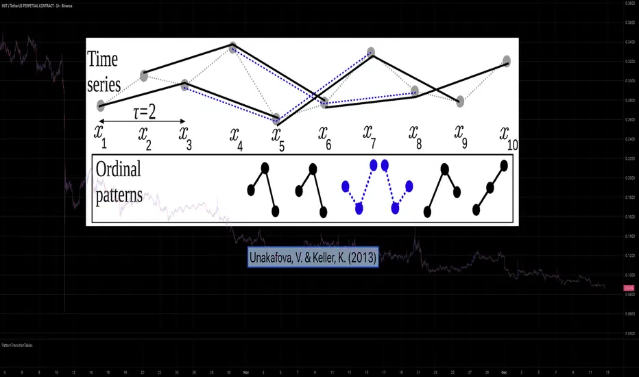
machine_learningLibrary "machine_learning"
euclidean(a, b)
Parameters:
a (array)
b (array)
manhattan(a, b)
Parameters:
a (array)
b (array)
cosine_similarity(a, b)
Parameters:
a (array)
b (array)
cosine_distance(a, b)
Parameters:
a (array)
b (array)
chebyshev(a, b)
Parameters:
a (array)
b (array)
minkowski(a, b, p)
Parameters:
a (array)
b (array)
p (float)
dot_product(a, b)
Parameters:
a (array)
b (array)
vector_norm(arr, p)
Parameters:
arr (array)
p (float)
sigmoid(x)
Parameters:
x (float)
sigmoid_derivative(x)
Parameters:
x (float)
tanh_derivative(x)
Parameters:
x (float)
relu(x)
Parameters:
x (float)
relu_derivative(x)
Parameters:
x (float)
leaky_relu(x, alpha)
Parameters:
x (float)
alpha (float)
leaky_relu_derivative(x, alpha)
Parameters:
x (float)
alpha (float)
elu(x, alpha)
Parameters:
x (float)
alpha (float)
gelu(x)
Parameters:
x (float)
swish(x, beta)
Parameters:
x (float)
beta (float)
softmax(arr)
Parameters:
arr (array)
apply_activation(arr, activation_type, alpha)
Parameters:
arr (array)
activation_type (string)
alpha (float)
normalize_minmax(arr, min_val, max_val)
Parameters:
arr (array)
min_val (float)
max_val (float)
normalize_zscore(arr, mean_val, std_val)
Parameters:
arr (array)
mean_val (float)
std_val (float)
normalize_matrix_cols(m)
Parameters:
m (matrix)
scaler_fit(arr, method)
Parameters:
arr (array)
method (string)
scaler_fit_matrix(m, method)
Parameters:
m (matrix)
method (string)
scaler_transform(scaler, arr)
Parameters:
scaler (ml_scaler)
arr (array)
scaler_transform_matrix(scaler, m)
Parameters:
scaler (ml_scaler)
m (matrix)
clip(x, lo, hi)
Parameters:
x (float)
lo (float)
hi (float)
clip_array(arr, lo, hi)
Parameters:
arr (array)
lo (float)
hi (float)
loss_mse(predicted, actual)
Parameters:
predicted (array)
actual (array)
loss_rmse(predicted, actual)
Parameters:
predicted (array)
actual (array)
loss_mae(predicted, actual)
Parameters:
predicted (array)
actual (array)
loss_binary_crossentropy(predicted, actual)
Parameters:
predicted (array)
actual (array)
loss_huber(predicted, actual, delta)
Parameters:
predicted (array)
actual (array)
delta (float)
gradient_step(weights, gradients, lr)
Parameters:
weights (array)
gradients (array)
lr (float)
adam_step(weights, gradients, m, v, lr, beta1, beta2, t, epsilon)
Parameters:
weights (array)
gradients (array)
m (array)
v (array)
lr (float)
beta1 (float)
beta2 (float)
t (int)
epsilon (float)
clip_gradients(gradients, max_norm)
Parameters:
gradients (array)
max_norm (float)
lr_decay(initial_lr, decay_rate, step)
Parameters:
initial_lr (float)
decay_rate (float)
step (int)
lr_cosine_annealing(initial_lr, min_lr, step, total_steps)
Parameters:
initial_lr (float)
min_lr (float)
step (int)
total_steps (int)
knn_create(k, distance_type)
Parameters:
k (int)
distance_type (string)
knn_fit(model, X, y)
Parameters:
model (ml_knn)
X (matrix)
y (array)
knn_predict(model, x)
Parameters:
model (ml_knn)
x (array)
knn_predict_proba(model, x)
Parameters:
model (ml_knn)
x (array)
knn_batch_predict(model, X)
Parameters:
model (ml_knn)
X (matrix)
linreg_fit(X, y)
Parameters:
X (matrix)
y (array)
ridge_fit(X, y, lambda)
Parameters:
X (matrix)
y (array)
lambda (float)
linreg_predict(model, x)
Parameters:
model (ml_linreg)
x (array)
linreg_predict_batch(model, X)
Parameters:
model (ml_linreg)
X (matrix)
linreg_score(model, X, y)
Parameters:
model (ml_linreg)
X (matrix)
y (array)
logreg_create(n_features, learning_rate, iterations)
Parameters:
n_features (int)
learning_rate (float)
iterations (int)
logreg_fit(model, X, y)
Parameters:
model (ml_logreg)
X (matrix)
y (array)
logreg_predict_proba(model, x)
Parameters:
model (ml_logreg)
x (array)
logreg_predict(model, x, threshold)
Parameters:
model (ml_logreg)
x (array)
threshold (float)
logreg_batch_predict(model, X, threshold)
Parameters:
model (ml_logreg)
X (matrix)
threshold (float)
nb_create(n_classes)
Parameters:
n_classes (int)
nb_fit(model, X, y)
Parameters:
model (ml_nb)
X (matrix)
y (array)
nb_predict_proba(model, x)
Parameters:
model (ml_nb)
x (array)
nb_predict(model, x)
Parameters:
model (ml_nb)
x (array)
nn_create(layers, activation)
Parameters:
layers (array)
activation (string)
nn_forward(model, x)
Parameters:
model (ml_nn)
x (array)
nn_predict_class(model, x)
Parameters:
model (ml_nn)
x (array)
accuracy(y_true, y_pred)
Parameters:
y_true (array)
y_pred (array)
precision(y_true, y_pred, positive_class)
Parameters:
y_true (array)
y_pred (array)
positive_class (int)
recall(y_true, y_pred, positive_class)
Parameters:
y_true (array)
y_pred (array)
positive_class (int)
f1_score(y_true, y_pred, positive_class)
Parameters:
y_true (array)
y_pred (array)
positive_class (int)
r_squared(y_true, y_pred)
Parameters:
y_true (array)
y_pred (array)
mse(y_true, y_pred)
Parameters:
y_true (array)
y_pred (array)
rmse(y_true, y_pred)
Parameters:
y_true (array)
y_pred (array)
mae(y_true, y_pred)
Parameters:
y_true (array)
y_pred (array)
confusion_matrix(y_true, y_pred, n_classes)
Parameters:
y_true (array)
y_pred (array)
n_classes (int)
sliding_window(data, window_size)
Parameters:
data (array)
window_size (int)
train_test_split(X, y, test_ratio)
Parameters:
X (matrix)
y (array)
test_ratio (float)
create_binary_labels(data, threshold)
Parameters:
data (array)
threshold (float)
lag_matrix(data, n_lags)
Parameters:
data (array)
n_lags (int)
signal_to_position(prediction, threshold_long, threshold_short)
Parameters:
prediction (float)
threshold_long (float)
threshold_short (float)
confidence_sizing(probability, max_size, min_confidence)
Parameters:
probability (float)
max_size (float)
min_confidence (float)
kelly_sizing(win_rate, avg_win, avg_loss, max_fraction)
Parameters:
win_rate (float)
avg_win (float)
avg_loss (float)
max_fraction (float)
sharpe_ratio(returns, risk_free_rate)
Parameters:
returns (array)
risk_free_rate (float)
sortino_ratio(returns, risk_free_rate)
Parameters:
returns (array)
risk_free_rate (float)
max_drawdown(equity)
Parameters:
equity (array)
atr_stop_loss(entry_price, atr, multiplier, is_long)
Parameters:
entry_price (float)
atr (float)
multiplier (float)
is_long (bool)
risk_reward_take_profit(entry_price, stop_loss, ratio)
Parameters:
entry_price (float)
stop_loss (float)
ratio (float)
ensemble_vote(predictions)
Parameters:
predictions (array)
ensemble_weighted_average(predictions, weights)
Parameters:
predictions (array)
weights (array)
smooth_prediction(current, previous, alpha)
Parameters:
current (float)
previous (float)
alpha (float)
regime_classifier(volatility, trend_strength, vol_threshold, trend_threshold)
Parameters:
volatility (float)
trend_strength (float)
vol_threshold (float)
trend_threshold (float)
ml_knn
Fields:
k (series int)
distance_type (series string)
X_train (matrix)
y_train (array)
ml_linreg
Fields:
coefficients (array)
intercept (series float)
lambda (series float)
ml_logreg
Fields:
weights (array)
bias (series float)
learning_rate (series float)
iterations (series int)
ml_nn
Fields:
layers (array)
weights (matrix)
biases (array)
weight_offsets (array)
bias_offsets (array)
activation (series string)
ml_nb
Fields:
class_priors (array)
means (matrix)
variances (matrix)
n_classes (series int)
ml_scaler
Fields:
min_vals (array)
max_vals (array)
means (array)
stds (array)
method (series string)
ml_train_result
Fields:
loss_history (array)
final_loss (series float)
converged (series bool)
iterations_run (series int)
ml_prediction
Fields:
class_label (series int)
probability (series float)
probabilities (array)
value (series float)
