Machine Learning Price Predictor: Ridge AR [Bitwardex]🔹Machine Learning Price Predictor: Ridge AR is a research-oriented indicator demonstrating the use of Regularized AutoRegression (Ridge AR) for short-term price forecasting.
The model combines autoregressive structure with Ridge regularization , providing stability under noisy or volatile market conditions.
The latest version introduces Bull and Bear signals , visually representing the current momentum phase and model direction directly on the chart.
Unlike traditional linear regression, Ridge AR minimizes overfitting, stabilizes coefficient dynamics, and enhances predictive consistency in correlated datasets.
The script plots:
Fit Line — in-sample fitted data;
Forecast Line — out-of-sample projection;
Trend Segments — color-coded bullish/bearish sections;
Bull/Bear Labels 🐂🐻 — dynamic visual signals showing directional bias.
Designed for researchers, students, and developers, this tool helps explore regularized time-series forecasting in Pine Script™.
🧩 Ridge AR Settings
Training Window — number of bars used for model training;
Forecast Horizon — forecast length (bars ahead);
AR Order — number of lags used as features;
Ridge Strength (λ) — regularization coefficient;
Damping Factor — exponential trend decay rate;
Trend Length — period for trend/volatility estimation;
Momentum Weight — strength of the recent move;
Mean Reversion — pullback intensity toward the mean.
🧮 Data Processing
Prefilter:
None — raw close price;
EMA — exponential smoothing;
SuperSmoother — Ehlers filter for noise reduction.
EMA Length, SuperSmoother Length — smoothing parameters.
🖥️ Display Settings
Update Mode:
Lock — static model;
Update Once Reached — rebuild after forecast horizon;
Continuous — update every bar.
Forecast Color — projection line color;
Bullish/Bearish Colors — colors for trend segments.
🐂🐻 Bull/Bear Signal System
The Bull/Bear Signal System adds directional visual cues to highlight local momentum shifts and model-based trend confirmation.
Bull (🐂) — appears when upward momentum is confirmed (momentum > 0) .
Displayed below the bar, colored with Bullish Color.
Bear (🐻) — appears when downward momentum is dominant (momentum < 0) .
Displayed above the bar, colored with Bearish Color.
Signals are generated during model recalculations or when the directional bias changes in Continuous mode.
These visual markers are analytical aids , not trading triggers.
🧠 Core Algorithmic Components
Regularized AutoRegression (Ridge AR):
Solves: (X′X+λI)−1X′y
to derive stable regression coefficients.
Matrix and Pseudoinverse Operations — implemented natively in Pine Script™.
Prefiltering (EMA / Ehlers SuperSmoother) — stabilizes noisy data.
Forecast Dynamics — integrates damping, momentum, and mean reversion.
Trend Visualization — color-coded bullish/bearish line segments.
Bull/Bear Signal Engine — visualizes real-time impulse direction.
📊 Applications
Academic and educational purposes;
Demonstration of Ridge Regression and AR models;
Analysis of bull/bear market phase transitions;
Visualization of time-series dependencies.
⚠️ Disclaimer
This script is provided for educational and research purposes only.
It does not provide trading or investment advice.
The author assumes no liability for financial losses resulting from its use.
Use responsibly and at your own risk.
Regressions

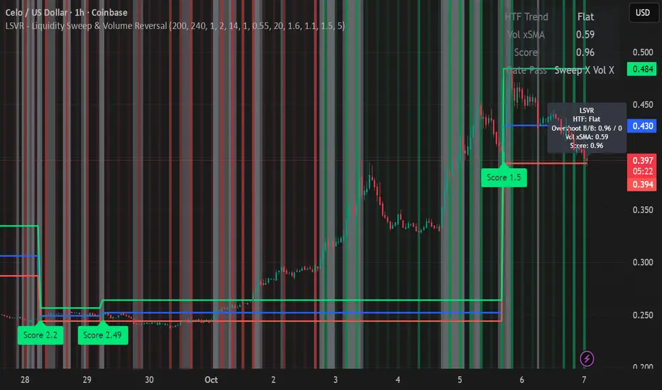
LSVR - Liquidity Sweep & Volume ReversalLSVR condenses a pro workflow into one visual overlay: Higher-Timeframe (HTF) Trend → Liquidity Sweep & Reclaim → Volume Confirmation. A signal only prints when all three gates align at bar close, and the chart shows everything you need—trend context, the sweep “trap” candle, and a projected Entry/SL/TP based on your chosen R multiple.
How it works
HTF Trend Filter: Projects a smoothed KAMA/EMA from a higher timeframe to the chart using a safe, lookahead-off request. Long signals are considered only above the HTF line; shorts only below.
Liquidity Sweep & Reclaim: Finds confirmed swing highs/lows, then detects an ATR-scaled overshoot through that swing followed by a reclaim (close back inside a configurable % of the bar range).
Volume Confirmation: Requires either a volume spike over Volume SMA × multiplier or optional OBV divergence. No participation = no signal.
Score: Each setup is scored: trend (0/1) + overshoot strength (0..1.5) + conviction (0/1). Signals fire only when the score ≥ Min Signal Score.
What you see
HTF Ribbon (subtle green/red backdrop) for bias.
Sweep Box on the signal candle (green = long, red = short).
Signal markers (“L” / “S”) with a small score label.
Projected lines that persist until the next signal: Entry (close), Stop (beyond swept swing), Target (R multiple).
Heatmap that intensifies when the score crosses your threshold.
Dashboard (top-right): HTF direction, Volume×SMA, current Score, gate pass status.
Tooltip on the last bar with quick stats.
Quick start
Apply to any liquid symbol and set HTF to ~3–6× your chart timeframe (e.g., 15m chart → 1H–4H).
Trade with the HTF trend: take L signals above the HTF line and S signals below it.
Entry = signal bar close, SL = beyond the swept swing, TP = your Projected Take-Profit (R).
Tighten or loosen selectivity with Min Signal Score, Reclaim %, Overshoot (ATR×), and Cooldown.
Recommended presets
Choppy/crypto 15m: minScore 1.25, reclaimPct 0.60–0.65, overshootATR 1.0–1.2, useOBVDiv=false, cooldown 8.
FX 5m / session trend: minScore 1.0–1.1, reclaimPct 0.50–0.55, overshootATR 0.8–1.0, useOBVDiv=true, cooldown 5.
Indices 1m (RTH): minScore 1.2, reclaimPct 0.55–0.60, useOBVDiv=false, cooldown 10.
Non-repainting by design
HTF values use lookahead_off with realtime offset.
Swings are confirmed pivots (no “forming” pivots).
Signals print at bar close only.
Notes
OBV divergence can add sensitivity on liquid markets; keep it off for stricter filtering.
Use Cooldown to avoid clustered sweeps.
This is an overlay/analysis tool, not financial advice. Test settings in Replay/Paper Trading before using live.
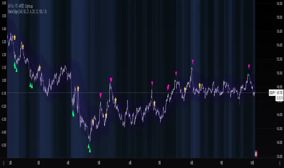
Stella Edge|SuperFundedStella Edge — Quick Guide
What it is
Stella Edge is a higher-timeframe (HTF) EMA + ATR channel with adaptive zones, a volatility hazard filter, and clean entry/exit cues. It projects an HTF EMA with ATR bands, paints a calm-to-active “aurora” background using normalized ATR, and marks:
・Long cue when price crosses up into/through the lower band (potential buy zone).
・Short cue when price crosses down into/through the upper band (potential sell zone).
・Take-profit star when price crosses back through the HTF EMA against your active direction.
・Skull marker on extreme volatility bars (ATR & Volume spikes) to warn of unstable conditions.
Why this is not a simple mashup
・HTF regime first: Instead of reacting to local noise, entries are contextualized by an HTF EMA±ATR envelope (request.security) that frames price with structural zones (upper = supply bias, lower = demand bias).
・Risk-aware gating: A dual-threshold volatility filter flags bars where true range and volume spike far above their baselines—conditions that often degrade signal quality.
・Signal hygiene: Cross checks use band values from the prior bar to reduce duplicate/ambiguous triggers when HTF data updates, yielding cleaner, fewer, higher-quality icons.
・Visual cognition: The aurora background blends two night tones by the percent-rank of HTF ATR, so your eye immediately senses regime intensity without reading numbers.
How it works (concise)
1. Pull HTF EMA(len) and HTF ATR(len) via request.security.
2. Compute upper/lower bands = EMA ± ATR×multiplier (projected continuously).
3. Aurora mode: Normalize HTF ATR by 200-bar percent-rank and map it to a calm→active gradient for background.
4. Signals
・Long when close crosses up the lowerBand .
・Short when close crosses down the upperBand .
・Track tradeDirection and print a ⭐️ when price crosses the HTF EMA against the current direction (TP cue).
5. Volatility hazard (optional): Flag bars where
・TR ≥ ATR(avg, N) × multiplier and
・Volume ≥ SMA(volume, M) × multiplier.
These get a 💀 label so you can avoid forced entries/exits during disorderly bursts.
Parameters (UI mapping)
Higher-Timeframe & Core
・Higher TF for EMA/ATR: HTF used by request.security (e.g., 60).
・EMA Length (HTF): HTF EMA period.
・ATR Length (HTF): HTF ATR period.
・ATR Multiplier: Band width.
・Aurora mode: Toggle dynamic background (ATR-based gradient).
Volatility Filter (Volatility Filter group)
・Enable Extreme Volatility Filter?: On/off.
・ATR Period / ATR Spike Multiplier: Bar is “extreme” if TR ≥ ATR×multiplier.
・Volume MA Period / Volume Spike Multiplier: “Extreme” also requires Volume ≥ SMA×multiplier.
Signal Settings
・Long Arrow Color / Short Arrow Color: Icon colors for long/short cues.
Practical usage
・Plan around the HTF envelope:
・Below lower band → price may be stretched into demand zone (look for long cue & reaction).
・Above upper band → stretched into supply zone (look for short cue & reaction).
・Confirmation: Treat arrows as triggers, not commands. Favor entry when you also see reaction candles (rejection wicks, engulfings) or micro-structure alignment.
・Exit discipline: The ⭐️ on EMA cross-back is a simple, mechanical TP. You can scale out earlier using fixed R-multiples or prior swing levels.
・Hazard bars: Avoid initiating on 💀 bars; widen stops or step aside until volatility normalizes.
・Clutter control: If zones feel too reactive, raise HTF (e.g., 120/240) or increase ATR Length/Multiplier for broader, slower bands.
Repainting & HTF notes
・HTF series from request.security are final only when the HTF bar closes. Using upperBand /lowerBand for crosses helps reduce duplicate/early prints, but intrabar behavior on the current HTF bar can still evolve. Evaluate on closed bars for strict confirmation.
Best markets & timeframes
・Pairs/indices/crypto where trend–pullback cycles are common.
・Start with entry TF = your usual trading TF (e.g., 5m–1h) and HTF = 3–12× that TF (e.g., 60/120/240).
・For BTC/Gold or newsy assets, prefer higher HTF and the volatility filter ON.
Disclaimer
This tool identifies zones and timing cues; it does not guarantee outcomes. News shocks and liquidity gaps can invalidate any setup. Always size positions prudently and trade at your own risk.
SuperFunded invite-only
To obtain access, please DM me on TradingView or use the link in my profile.
Stella Edge — クイックガイド(日本語)
概要
Stella Edgeは、上位足EMA±ATRバンドで相場をフレーミングし、アダプティブな買い/売りゾーン、極端なボラティリティ警告、そしてシンプルなエントリー/利確キューを提供するインジです。
・ロング:価格が Lower Bandを上抜けたタイミングで矢印。
・ショート:価格が Upper Bandを下抜けたタイミングで矢印。
・利確⭐️:建玉方向に対して価格が HTF EMA を逆行クロスしたら表示。
・💀警告:ATRと出来高が同時スパイクした「危険」バーを明示。
・背景はHTF ATRのパーセントランクで静→動にグラデーションする「オーロラ」表現。
独自性・新規性
・上位足の構造を先に定義(EMA±ATR)→そこへ戻る/抜ける動きだけを狙うため、ノイズを減らした文脈型の判断が可能。
・二重スパイク条件(TR×ATR基準+出来高×SMA基準)で、荒れ相場のエントリー回避を支援。
・シグナルの重複・不安定を抑制、見やすい最小限のアイコンに整理。
・視覚設計としてATRの相対的な強度を背景で可視化し、一目で局面認識。
使い方のヒント
・ゾーンは押し目/戻り目の候補。矢印はトリガーとして扱い、ローソクの反応(ピンバー/包み足など)で確認してから入る。
・⭐️は機械的TPの目安。スケールアウトやR倍数での利確も併用可。
・💀が出た足での新規は原則回避。HTFを上げるとゾーンはより鈍感=落ち着いた絵に。
・HTF更新の注意:上位足バー確定までは値が変化し得ます。確定足ベースで検証するのが安全。
免責
本ツールは反発や到達を保証しません。イベントや流動性によって機能しないことがあります。資金管理のもと自己責任でご利用ください。
SuperFunded 招待専用スクリプト
このスクリプトはSuperFundedの参加者専用です。アクセスをご希望の方は、SuperFundedにご登録のメールアドレスから partner@superfunded.com 宛に、TradingViewの登録名をご送信ください。
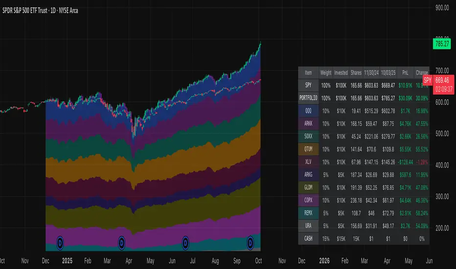
Normalized Portfolio TrackerThis script lets you create, visualize, and track a custom portfolio of up to 15 assets directly on TradingView.
It calculates a synthetic "portfolio index" by combining multiple tickers with user-defined weights, automatically normalizing them so the total allocation always equals 100%.
All assets are scaled to a common starting point, allowing you to compare your portfolio’s performance versus any benchmark like SPY, QQQ, or BTC.
🚀 Goal
This script helps traders and investors:
• Understand the combined performance of their portfolio.
• Normalize diverse assets into a single synthetic chart .
• Make portfolio-level insights without relying on external spreadsheets.
🎯 Use Cases
• Backtest your portfolio allocations directly on the chart.
• Compare your portfolio vs. benchmarks like SPY, QQQ, BTC.
• Track thematic baskets (commodities, EV supply chain, regional ETFs).
• Visualize how each component contributes to overall performance.
📊 Features
• Weighted Portfolio Performance : Combines selected assets into a synthetic value series.
• Base Price Alignment : Each asset is normalized to its starting price at the chosen date.
• Dynamic Portfolio Table : Displays symbols, normalized weights (%), equivalent shares (based on each asset’s start price, sums to 100 shares), and a total row that always sums to 100%.
• Multi-Asset Support : Works with stocks, ETFs, indices, crypto, or any TradingView-compatible symbol.
⚙️ Configuration
Flexible Portfolio Setup
• Add up to 15 assets with custom weight inputs.
• You can enter any arbitrary numbers (e.g. 30, 15, 55).
• The script automatically normalizes all weights so the total allocation always equals 100%.
Start Date Selection
• Choose any custom start date to normalize all assets.
• The portfolio value is then scaled relative to the main chart symbol, so you can directly compare portfolio performance against benchmarks like SPY or QQQ.
Chart Styles
• Candlestick chart
• Heikin Ashi chart
• Line chart
Custom Display
• Adjustable colors and line widths
• Optionally display asset list, normalized weights, and equivalent shares
⚙️ How It Works
• Fetch OHLC data for each asset.
• Normalizes weights internally so totals = 100%.
• Stores each asset’s base price at the selected start date.
• Calculates equivalent “shares” for each allocation.
• Builds a synthetic portfolio value series by summing weighted contributions.
• Renders as Candlestick, Heikin Ashi, or Line chart.
• Adds a portfolio info table for clarity.
⚠️ Notes
• This script is for visualization only . It does not place trades or auto-rebalance.
• Weight inputs are automatically normalized, so you don’t need to enter exact percentages.
Regression Channel (ShareScope-style, parallel)What it does
Replicates ShareScope’s Trend of displayed data look: a single straight linear-regression line (dashed) across a chosen window with parallel, constant-width bands above and below, plus optional shading.
Use it to see the overall trend gradient for a period and a statistically sized channel based on the fit’s residual error.
How it works (math, short)
Computes an OLS regression once over the analysis window.
Residual standard error s is derived from SSE and degrees of freedom (n−2).
Band half-width is constant across the window:
Mean CI (narrower): half = z * s / √n
Prediction (wider): half = z * s * √(1 + 1/n)
Three straight, parallel lines are drawn from the regression endpoints; midline is dashed.
This is intentionally not a tapered CI (which widens at the ends). It matches the visual behaviour of ShareScope’s shaded trend line channel.
Inputs
Source – Price series (Close, High, Low, HL2, etc.).
Use last N bars / N (bars) – Rolling window length.
From / To (date mode) – Alternative fixed date window.
Confidence (%) – 90 / 95 / 99 / Custom (uses z≈t).
Custom Z (t) – Override the quantile if desired.
Prediction bands – Use wider prediction envelope instead of mean CI.
Shade region + colors / opacity / line width.
Usage
To mimic ShareScope exactly, pick the same date span (use date mode) and set Confidence 99%.
Choose Prediction OFF for a tighter “confidence” look; ON for a wider, more permissive channel.
If ShareScope used High as source, set Source = High here as well.
Notes & limitations
TradingView does not expose the visible viewport to Pine. The script cannot auto-read “displayed data.” Use last N bars or date range.
Bands are parallel by design. Prices may close outside; the channel does not bend.
Window capped at 5,000 bars for performance. No alerts are emitted.
Differences vs TV’s native tools
Linear Regression (drawing) – manual object; no statistical sizing or shading.
Linear Regression Channel (indicator) – uses price standard deviations around the regression; width is a user stdev multiple.
This script – uses residual error of the OLS fit and a z/t quantile to size a statistically meaningful parallel channel.
Changelog
r3.1 – Guard fix (no return at top level), minor refactor, stable line updates.
r3 – Switched to single-fit OLS with parallel constant-width bands (ShareScope look).
(Earlier experimental builds r1–r2.2 implemented rolling/tapered CI; superseded.)
Disclaimer: Educational use only. Not investment advice.

Linear Regression by Uttamwith Buy Sell Signal with regression channel
with Buy Sell Signal with regression channel
with Buy Sell Signal with regression channel
with Buy Sell Signal with regression channel

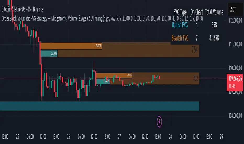
Order Block Volumatic FVG StrategyInspired by: Volumatic Fair Value Gaps —
License: CC BY-NC-SA 4.0 (Creative Commons Attribution–NonCommercial–ShareAlike).
This script is a non-commercial derivative work that credits the original author and keeps the same license.
What this strategy does
This turns BigBeluga’s visual FVG concept into an entry/exit strategy. It scans bullish and bearish FVG boxes, measures how deep price has mitigated into a box (as a percentage), and opens a long/short when your mitigation threshold and filters are satisfied. Risk is managed with a fixed Stop Loss % and a Trailing Stop that activates only after a user-defined profit trigger.
Additions vs. the original indicator
✅ Strategy entries based on % mitigation into FVGs (long/short).
✅ Lower-TF volume split using upticks/downticks; fallback if LTF data is missing (distributes prior bar volume by close’s position in its H–L range) to avoid NaN/0.
✅ Per-FVG total volume filter (min/max) so you can skip weak boxes.
✅ Age filter (min bars since the FVG was created) to avoid fresh/immature boxes.
✅ Bull% / Bear% share filter (the 46%/53% numbers you see inside each FVG).
✅ Optional candle confirmation and cooldown between trades.
✅ Risk management: fixed SL % + Trailing Stop with a profit trigger (doesn’t trail until your trigger is reached).
✅ Pine v6 safety: no unsupported args, no indexof/clamp/when, reverse-index deletes, guards against zero/NaN.
How a trade is decided (logic overview)
Detect FVGs (same rules as the original visual logic).
For each FVG currently intersected by the bar, compute:
Mitigation % (how deep price has entered the box).
Bull%/Bear% split (internal volume share).
Total volume (printed on the box) from LTF aggregation or fallback.
Age (bars) since the box was created.
Apply your filters:
Mitigation ≥ Long/Short threshold.
Volume between your min and max (if enabled).
Age ≥ min bars (if enabled).
Bull% / Bear% within your limits (if enabled).
(Optional) the current candle must be in trade direction (confirm).
If multiple FVGs qualify on the same bar, the strategy uses the most recent one.
Enter long/short (no pyramiding).
Exit with:
Fixed Stop Loss %, and
Trailing Stop that only starts after price reaches your profit trigger %.
Input settings (quick guide)
Mitigation source: close or high/low. Use high/low for intrabar touches; close is stricter.
Mitigation % thresholds: minimal mitigation for Long and Short.
TOTAL Volume filter: skip FVGs with too little/too much total volume (per box).
Bull/Bear share filter: require, e.g., Long only if Bull% ≥ 50; avoid Short when Bull% is high (Short Bull% max).
Age filter (bars): e.g., ≥ 20–30 bars to avoid fresh boxes.
Confirm candle: require candle direction to match the trade.
Cooldown (bars): minimum bars between entries.
Risk:
Stop Loss % (fixed from entry price).
Activate trailing at +% profit (the trigger).
Trailing distance % (the trailing gap once active).
Lower-TF aggregation:
Auto: TF/Divisor → picks 1/3/5m automatically.
Fixed: choose 1/3/5/15m explicitly.
If LTF can’t be fetched, fallback allocates prior bar’s volume by its close position in the bar’s H–L.
Suggested starting presets (you should optimize per market)
Mitigation: 60–80% for both Long/Short.
Bull/Bear share:
Long: Bull% ≥ 50–70, Bear% ≤ 100.
Short: Bull% ≤ 60 (avoid shorting into strong support), Bear% ≥ 0–70 as you prefer.
Age: ≥ 20–30 bars.
Volume: pick a min that filters noise for your symbol/timeframe.
Risk: SL 4–6%, trailing trigger 1–2%, distance 1–2% (crypto example).
Set slippage/fees in Strategy Properties.
Notes, limitations & best practices
Data differences: The LTF split uses request.security_lower_tf. If the exchange/data feed has sparse LTF data, the fallback kicks in (it’s deliberate to avoid NaNs but is a heuristic).
Real-time vs backtest: The current bar can update until close; results on historical bars use closed data. Use “Bar Replay” to understand intrabar effects.
No pyramiding: Only one position at a time. Modify pyramiding in the header if you need scaling.
Assets: For spot/crypto, TradingView “volume” is exchange volume; in some markets it may be tick volume—interpret filters accordingly.
Risk disclosure: Past performance ≠ future results. Use appropriate position sizing and risk controls; this is not financial advice.
Credits
Visual FVG concept and original implementation: BigBeluga.
This derivative strategy adds entry/exit logic, volume/age/share filters, robust LTF handling, and risk management while preserving the original spirit.
License remains CC BY-NC-SA 4.0 (non-commercial, attribution required, share-alike).
ML+MA+ATRretardretardretardretardretardretardretardretardretardretardretardretardretardretardretardretardretardretardretardretard never believe this
EMA Separation (LFZ Scalps) v6 — Early TriggerPlots the percentage distance between a fast and a slow EMA (default 9 & 21) to gauge trend strength and filter out choppy London Flow Zone breakouts.
• Gray – EMAs nearly flat (low momentum, avoid trades)
• Orange – early trend building
• Green/Red – strong directional momentum
Useful for day-traders: wait for the gap to widen beyond your chosen threshold (e.g., 0.25 %) before entering a breakout. Adjustable EMA lengths and alert when the separation exceeds your “strong trend” level.

Nadaraya-Watson Multi-TF DashboardThis script is a Multi-Timeframe Flip State Dashboard based on Nadaraya-Watson: Rational Quadratic Kernel (Non-Repainting) indicator. It visualizes trend "flip" states across up to 8 custom timeframes using a consistent, non-repainting methodology. Built on 1-minute data, each timeframe row in the table updates only after its bar fully closes, ensuring accuracy and eliminating repainting issues.
Key features:
✅ Based on the Nadaraya-Watson Rational Quadratic Kernel, used to estimate trend direction
🧠 Each timeframe uses the same base 1-minute data for consistency across resolutions
🔄 Flip state detection is defined by slope reversals in the kernel regression
🧱 Fully supports non-repainting, close-confirmed states using lookahead=off
🧮 Configurable lookback window, kernel weighting, lag, and timeframes
🎨 Visual dashboard plots each TF’s state as a colored cell (green for bullish, red for bearish)
🛠️ Includes inline plots and debug traces to help visualize regression and flip logic
This dashboard is ideal for traders who want a compact visual overview of confirmed trend shifts across multiple timeframes, all using a mathematically grounded, TF-consistent model.

JessieOBS with MACD - The Evil MACD 3.0中文版说明在后面
JessieOBS takes the classic MACD to the next level by clearly highlighting overbought and oversold zones.
While the traditional MACD works well for spotting uptrends and downtrends, it often struggles in sideways markets—producing false signals and useless crossovers that can trigger unnecessary stop losses. JessieOBS solves this problem, giving you cleaner, more reliable signals even when the market is moving sideways.
The thick red line signals an oversold area, hinting that a price reversal to an uptrend may happen soon.
The thick blue line signals an overbought area, hinting that a price reversal to a downtrend may happen soon.
JessieOBS helps you filter sideways trends, improving your win rate.
WARNING: JessieOBS is only an early WARNING, NOT A TRADE ENTRY SIGNAL.
When a warning appears, stay alert and wait for confirmation—through price action, divergences , or the theory of entanglement.
With the right approach, JessieOBS can take your win rate to the next level!
JessieOBS 3.0 – Update Highlights
New Feature: Automatic Divergence Detection
To enhance the effectiveness of JessieOBS, version 3.0 introduces automatic divergence marking. Using divergence alongside JessieOBS can improve win rates and help pinpoint potential reversal points more accurately.
1. Focused on MACD Histogram Divergence
Only the MACD histogram is used for divergence detection; the MACD divergences are not marked. This is because JessieOBS is a leading indicator, and the MACD lines and histogram convey different information:
MACD Line: Represents the overall trend and changes more gradually.
MACD Histogram: Reflects direction and momentum, changing more quickly.
Since JessieOBS is designed for early warning signals, observing divergence on the histogram allows for more precise detection of potential reversals.
2. How JessieOBS Divergence Differs from Other Indicators
Most divergence indicators on the market rely on future functions to repaint signals. This is necessary because a peak or trough can only be confirmed after it has formed. As a result, these indicators often repaint continuously until the last signal is fixed.
In JessieOBS, key divergence lines are preserved, allowing you to clearly track how signals evolved in real time, rather than retrospectively identifying tops or bottoms after the fact.
3. Usage Notes
Divergence lines may repaint and should be used as reference and alerts only. Rest assured, the core JessieOBS signals do not repaint or shift—they remain stable and reliable.
4. Interpreting Divergence Strength
Stronger Divergence: Larger price differences between two points create steeper divergence lines, indicating a more significant signal.
Weaker Divergence: Smaller price differences produce flatter lines, suggesting a milder and less impactful signal.
中文版说明:
传统的MACD可以很明确识别出趋势,但有两个最大的缺点:第一是滞后性,第二是假信号。所以MACD在趋势行情里比较好用(不管是上升趋势还是下降趋势),但在横盘期间,就会产生很多的假信号。
JessieOBS就解决了MACD不准的问题,在MACD的信号线上,添加了白色和蓝色的粗线,红色粗线代表价格超卖,接下来很可能会反转上涨,蓝色粗线代表价格超买,接下来很可能会反转下跌。市场横盘期间,JessieOBS很少会给出超买或者超卖信号,从而有效过滤了MACD的假信号。
注意!JessieOBS只能作为一个提前的预警,一定不能把JessieOBS当做入场信号看待。因为JessieOBS只预警价格可能会反转,但并不能预测出价格发生反转的准确时间。
正确的做法是,一旦看见JessieOBS的预警信号,就应该重点关注,再用其他的方式找到准确的入场点。裸k交易法是有用的,找到反转的趋势k线作为入场点。
强烈推荐:出现预警信号之后根据背离点入场,这种方法的胜率不错。
强烈推荐:出现预警信号之后根据缠论分析入场,利用缠论分析出的入场点胜率可以更高。
JessieOBS 3.0 更新说明
新加入功能:背离自动标注
在使用JessieOBS的过程中,结合背离会提高胜率,以及更精准找到反转点,所以在指标中加入了自动标注背离的功能。
1 没有标注MACD线的背离,只计算了MACD histogram部分背离,因为JessieOBS是一个左侧指标,但MACD线和柱状图代表的含义不同:
fastMA = f_calcMA(Source, Period, Type)
slowMA=f_calcMA(Source, Period, Type)
macdLine = fastMA - slowMA
signalLine=f_calcMA(macdLine,Period,Type)
macdHist = macdLine - signalLine
MACD线代表趋势,变化更慢,MACD histogram代表方向和力度,变化更快。
JessieOBS本身就是一个左侧指标,属于提前预警,那就应该观察柱状图的背离,这样才能更精确。
2 和市场上常见背离指标的区别:
其他背离指标,一般会用一个未来函数重绘图形,注意,涉及到背离的判断一定会用到未来函数,因为一个顶只有走出来了,你才能判断这是一个顶,否则就还有可能继续往上延伸,因为这一点逻辑本身的原因,所以背离一定会用到未来函数。
其他指标在连续背离发生的时候,一般都会不断重绘图形,直到保留最后一个信号的位置。
我在写背离的过程中,保留了一些主要的线段,这样就可以更清晰看见当时的演变过程,而不是站在事后的上帝视角回头去找一个确定的底或顶。
3 使用过程中,背离线因为有重绘的功能,所以只能用于参考和提醒,JessieOBS的信号仍然没有重绘和漂移,请放心使用。
4 背离的程度判定:两点价差越大,背离线的斜率越大,就可以判断背离越明显,这个背离的指导意义就越大;相反,两点价差越小,背离线的斜率越小,就可以判断背离越轻微,这个背离的指导意义就越小。

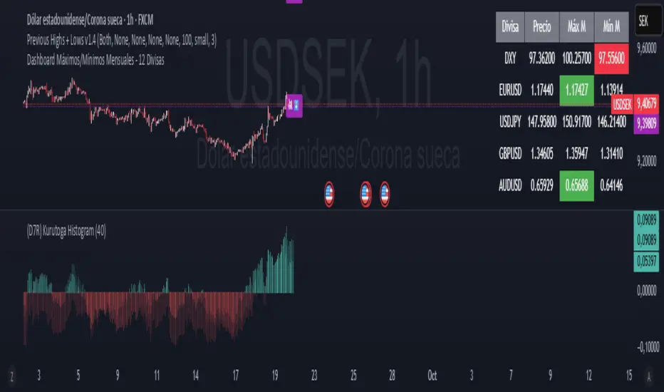
Dashboard Máximos/Mínimos Mensuales - 12 Divisas El ArconteMáximos y mínimos mensuales de doce divisas principales de FOREX.
Alerta de toque de la 200-Week SMACuando el precio toca la MMS de 200 semanas es una posible compra.

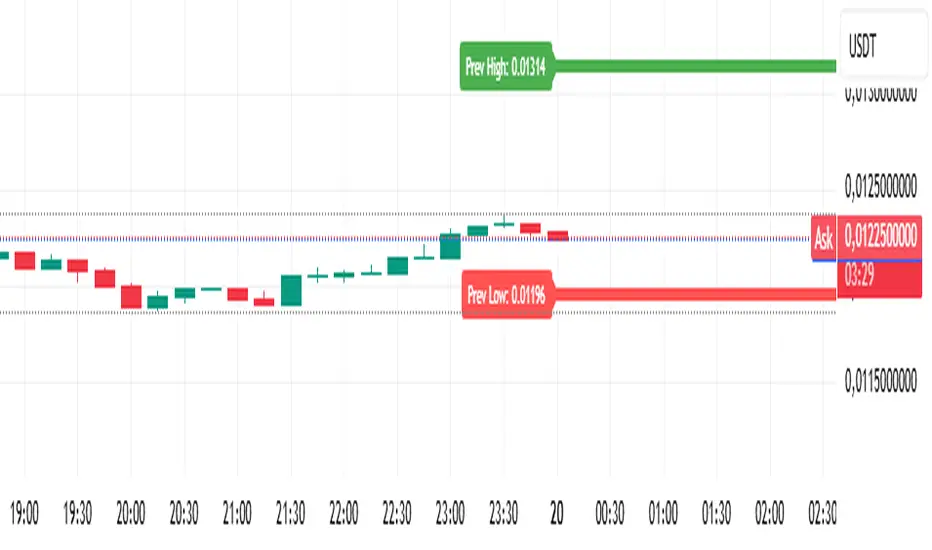
Analitica Trading — Previous Day SR (2 lines + labels) 2.0📊 Analitica Trading — Previous Day SR (Support & Resistance)
This indicator displays the previous day’s key levels on any timeframe:
Prev High → Green horizontal line with label.
Prev Low → Red horizontal line with label.
🔹 Stable across timeframes: The levels are calculated from the daily candles and remain fixed, no matter if you switch to 1D, 1H, or 5m.
🔹 Simple & clean: Exactly two lines only (no duplicates).
🔹 Price labels included: Each line has a clear tag showing the exact level.
🔹 Dynamic update: Lines refresh automatically at the start of each new daily session.
🔹 Alerts: Optional alerts trigger when the price breaks above the Prev High or below the Prev Low.
💡 Ideal for support/resistance trading, breakouts, and Smart Money Concepts (SMC) strategies.
MC RSI + Stoch (multi-level bands)This indicator combines RSI and Stochastic Oscillator into a single panel for easier market analysis. It is designed for traders who want both momentum context and precise timing, with multiple reference levels for better decision-making.
🔧 Features
RSI (Relative Strength Index) with adjustable length (default 14).
Stochastic Oscillator (default 18, 9, 5) with smoothing applied to %K.
Both oscillators plotted in the same scale (0–100) for clear comparison.
Custom horizontal levels:
10 & 90 (purple)
20 & 80 (teal)
30 & 70 (blue)
40 & 60 (gray)
50 midline (red) for balance point reference.
Optional shaded band between 20–80 for quick visualization of momentum extremes.
Toggle switches to show/hide RSI or Stochastic independently.
🎯 How to Use
RSI gives the overall momentum strength.
Stochastic provides faster entry/exit signals by showing short-term momentum shifts.
Use the multi-level bands to identify different market conditions:
10/90 = Extreme exhaustion zones.
20/80 = Overbought/oversold boundaries.
30/70 = Secondary confirmation levels.
40/60 = Neutral momentum bands.
50 = Midline equilibrium.
Omega ATR Indicator📖 Introduction
The Ω ATR Indicator was created to provide a more complete and professional framework for volatility analysis than the classic Average True Range (ATR).
While the traditional ATR is a useful tool, it has limitations: it delivers a simple rolling average of volatility, but it does not adapt to market regimes, it does not highlight extreme events, and it often leaves the trader with incomplete information about risk.
The Ω ATR takes the same foundation and elevates it into a multi-dimensional volatility dashboard, adding statistical layers, adaptive calculations, and clear visual references that allow traders to interpret volatility in a way that is immediately actionable.
🔎 What makes it different from a standard ATR?
This indicator introduces several features beyond the classic formula:
True Range Core – plots the raw True Range (TR) for each bar, providing a direct, bar-by-bar view of volatility impulses.
Standard & Adjusted ATR – includes both the conventional ATR (smoothed average) and an Adjusted ATR that automatically corrects for extreme conditions by incorporating percentile rescaling.
Percentile Volatility Levels – dynamically calculated extreme thresholds (99.8%, 75%, 50%, 25%), plotted as dotted levels across the chart. These act as reference lines for “normal” vs. “abnormal” volatility, useful for spotting unusual price expansions or contractions.
Linear Regression Volatility Trend – overlays a regression line of volatility, showing whether the market is moving toward expansion (rising vol), contraction (falling vol), or stability.
Monetary Value Translation – the indicator converts volatility into points, ticks, and dollar values (based on the instrument’s point value). This allows futures traders and high-value instruments users to immediately see how much volatility is “worth” in cash terms.
Interactive Table Display – a real-time statistics table is displayed directly on the chart, showing:
SMA of ATR in $ and points
Percentile-based volatility range (VAR) in $ and points
Tick equivalences, for quick position sizing
⚡ How traders can use it
The Ω ATR Indicator is designed to be versatile, fitting both discretionary traders and systematic strategy developers.
Risk Management: ATR-based stop losses and position sizing are significantly improved by using the adjusted ATR and percentile thresholds. Traders can size their positions according to volatility regimes, not just raw averages.
Breakout & Exhaustion Detection: When TR or ATR values spike above the 99.8% or 95% percentile levels, this often corresponds to breakout conditions or volatility exhaustion — useful for breakout strategies, mean-reversion setups, and volatility fades.
Market Regime Identification: The regression line helps distinguish if volatility is rising (trending environment, larger swings expected) or compressing (range-bound environment, lower risk opportunities).
Multi-Asset Flexibility: Works equally well on equities, futures, crypto, and FX. Its point/tick/dollar conversion makes it especially powerful for futures traders who need to quantify risk precisely.
Scalping to Swing Trading: On lower timeframes, it acts as a micro-volatility detector; on higher timeframes, it functions as a strategic risk gauge for position management.
⚙️ Settings and Customization
Length: The ATR lookback period (default = 34).
Shorter lengths (14–21) for intraday traders who want fast response.
Longer lengths (34–55) for swing/position traders who want smoother readings.
AVG / ADJ AVG: Toggle to display the standard ATR or the adjusted ATR.
Volatility Levels: Enable/disable up to 4 percentile-based levels (1st = 25%, 2nd = 50%, 3rd = 75%, 4th = 99.8%). Recommended: keep 3 levels active for clarity.
Color Controls: All plots and levels are fully customizable to match your chart style.
Table Display: Positioned on the chart (default: middle-right) with key values updated in real time.
🧭 Best Practices for Use
Combine with Trend Tools: Volatility readings are most powerful when combined with trend filters or volume analysis. For example, a breakout with both high volatility and trend confirmation is stronger than either alone.
ATR Stops: Use the Adjusted ATR rather than the standard one when trailing stops in highly volatile instruments like crypto or Nasdaq futures, as it adapts to outlier spikes.
Dollar Risk Translation: Use the dollar-value outputs to predefine maximum acceptable risk per trade (e.g., “I only risk $250 per position”). This bridges volatility to portfolio risk management.
Event Monitoring: Around economic events or earnings, expect volatility spikes above higher percentile levels. The indicator makes these moves instantly visible.
📌 Summary
The Ω ATR Indicator is not just “another ATR.” It is a comprehensive volatility framework that transforms volatility from a simple statistic into an actionable trading signal.
By combining:
the classic ATR,
an adjusted ATR,
percentile extremes,
regression-based volatility trends,
and real-time dollar conversions,
…this tool allows traders to precisely understand, visualize, and act on volatility in ways that a standard ATR simply cannot provide.
Whether you are scalping intraday moves, swing trading equities, or managing futures positions, the Ω ATR equips you with a professional-grade volatility dashboard that clarifies risk, highlights opportunity, and adapts across all markets and timeframes.
👉 Designed and developed by OmegaTools for traders who demand precision, clarity, and adaptability in their volatility analysis.

BTCUSD Dual Thrust (1H)BTCUSD Dual Thrust (1H) — Indicator
Overview
The Dual Thrust is a classic breakout-type strategy designed to capture strong directional moves when markets show imbalance between buyers and sellers. This indicator adapts the method specifically for BTCUSD on the 1-Hour timeframe, showing dynamic Buy/Sell trigger levels and live signals.
Origin
The Dual Thrust system was originally introduced by Michael Vitucci and has been widely used in futures and high-volatility markets. It was designed as a day-trading breakout framework, where daily high/low and close data define the range for the next session’s trade triggers.
How it Works
Each new day, the indicator calculates a “breakout range” using daily price data.
Two trigger levels are projected from the daily open:
Buy Trigger: Open + Range × KUp
Sell Trigger: Open - Range × KDn
Range can be built from either:
Classic Dual Thrust formula: max(High - Close , Close - Low) over a lookback period, or
ATR-based range: for volatility-adaptive signals.
A LONG signal fires when price crosses above the Buy Trigger.
An EXIT signal fires when price crosses below the Sell Trigger.
Buy/Sell lines step forward across each intraday bar until recalculated at the next daily open.
Practical Use
Optimized for BTCUSD 1-Hour charts (crypto’s volatility provides stronger follow-through).
Use the Buy/Sell levels as dynamic breakout lines or as confluence with your own setups.
Alerts are built in, so you can receive notifications when a LONG or EXIT condition triggers.
Designed as an indicator only (not a backtest strategy).
Key Features
✅ Daily Buy/Sell trigger lines auto-calculated and forward-filled
✅ LONG / EXIT labels on signals
✅ Optional ATR mode for volatility regimes
✅ Optional bar coloring for easy visual scanning
✅ Alerts ready for live monitoring
⚡️ Tip: While this indicator highlights breakout opportunities, effectiveness can improve when combined with trend filters (e.g., 200-SMA) or when aligned with higher timeframe supply/demand zones.

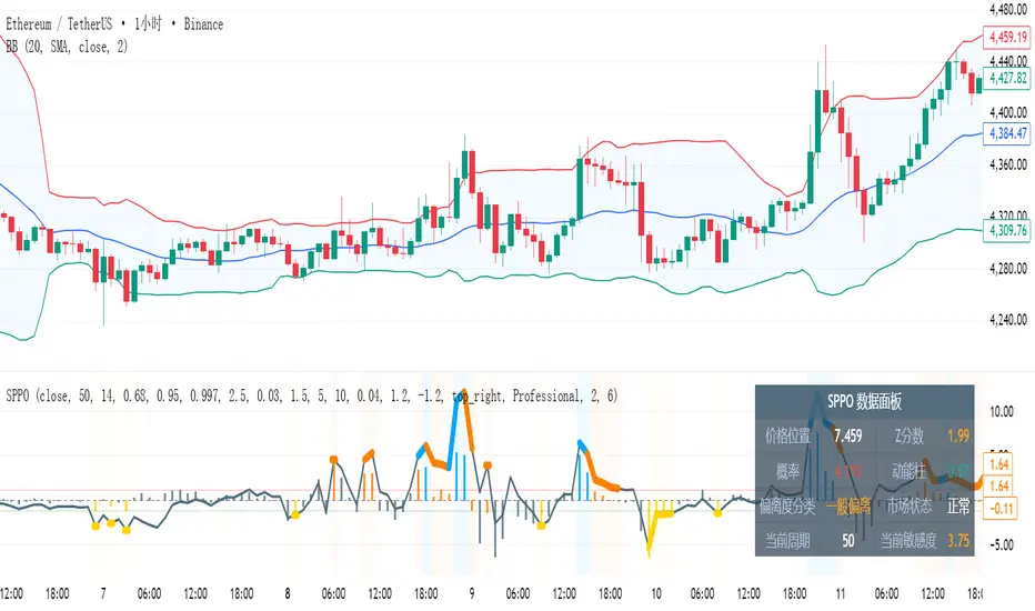
SPPO - Statistical Price Position OscillatorSPPO - Statistical Price Position Oscillator - Time-Weighted
Based on a time-weighted statistical model, this indicator quantifies price deviation from its recent mean. It uses a Z-Score to normalize price position and calculates the statistical probability of its occurrence, helping traders identify over-extended market conditions and mean-reversion opportunities with greater sensitivity.
- Time-Weighted Model: Reacts more quickly to recent price changes by using a Weighted Moving Average (WMA) and a weighted standard deviation.
- Statistical Foundation: Utilizes Z-Score standardization and a probability calculation to provide an objective measure of risk and price extremity.
- Dynamic Adaptation: Automatically adjusts its calculation period and sensitivity based on market volatility, making it versatile across different market conditions.
- Intelligent Visuals: Dynamic line thickness and gradient color-coding intuitively display the intensity of price deviations.
- Multi-Dimensional Analysis: Combines the main line's position (Z-Score), a momentum histogram, and real-time probability for a comprehensive view.
1. Time-Weighted Statistical Model (Z-Score Calculation)
- Weighted Mean (μ_w): Instead of a simple average, the indicator uses a Weighted Moving Average (ta.wma) to calculate the price mean, giving more weight to recent data points.
- Weighted Standard Deviation (σ_w): A custom weighted_std function calculates the standard deviation, also prioritizing recent prices. This ensures that the measure of dispersion is more responsive to the latest market behavior.
- Z-Score: The core of the indicator is the Z-Score, calculated as Z = (Price - μ_w) / σ_w. This value represents how many weighted standard deviations the current price is from its weighted mean. A higher absolute Z-Score indicates a more statistically significant price deviation.
2. Probability Calculation
- The indicator uses an approximation of the Normal Cumulative Distribution Function (normal_cdf_approx) to calculate the probability of a Z-Score occurring.
- The final price_probability is a two-tailed probability, calculated as 2 * (1 - CDF(|Z-Score|)). This value quantifies the statistical rarity of the current price deviation. For example, a probability of 0.05 (or 5%) means that a deviation of this magnitude or greater is expected to occur only 5% of the time, signaling a potential market extreme.
3. Dynamic Parameter Adjustment
- Volatility Measurement: The system measures market volatility using the standard deviation of price changes (ta.stdev(ta.change(src))) over a specific lookback period.
- Volatility Percentile: It then calculates the percentile rank (ta.percentrank) of the current volatility relative to its history. This contextualizes whether the market is in a high-volatility or low-volatility state.
- Adaptive Adjustment:
- If volatility is high (e.g., >75th percentile), the indicator can shorten its distribution_period and increase its position_sensitivity. This makes it more responsive to fast-moving markets.
- If volatility is low (e.g., <25th percentile), it can lengthen the period and decrease sensitivity, making it more stable in calmer markets. This adaptive mechanism helps maintain the indicator's relevance across different market regimes.
4. Momentum and Cycle Analysis (Histogram)
- The indicator does not use a Hilbert Transform. Instead, it analyzes momentum cycles by calculating a histogram: Histogram = (Z-Score - EMA(Z-Score)) * Sensitivity.
- This histogram represents the rate of change of the Z-Score. A positive and rising histogram indicates accelerating upward deviation, while a negative and falling histogram indicates accelerating downward deviation. Divergences between the price and the histogram can signal a potential exhaustion of the current deviation trend, often preceding a reversal.
- Reversal Signals: Look for the main line in extreme zones (e.g., Z-Score > 2 or < -2), probability below a threshold (e.g., 5%), and divergence or contraction in the momentum histogram.
- Trend Filtering: The main line's direction indicates the trend of price deviation, while the histogram confirms its momentum.
- Risk Management: Enter a high-alert state when probability drops below 5%; consider risk control when |Z-Score| > 2.
- Gray, thin line: Price is within a normal statistical range (~1 sigma, ~68% probability).
- Orange/Yellow, thick line: Price is moderately deviated (1 to 2 sigma).
- Cyan/Purple, thick line: Price is extremely deviated (>2 sigma, typically <5% probability).
- Distribution Period: 50 (for weighted calculation)
- Position Sensitivity: 2.5
- Volatility Lookback: 10
- Probability Threshold: 0.03
Suitable for all financial markets and timeframes, especially in markets that exhibit mean-reverting tendencies.
This indicator is a technical analysis tool and does not constitute investment advice. Always use in conjunction with other analysis methods and a strict risk management strategy.
Copyright (c) 2025 | Pine Script v6 Compatible
---
统计价格位置振荡器 (SPPO) - 时间加权版
基于时间加权统计学模型,该指标量化了当前价格与其近期均值的偏离程度。它使用Z分数对价格位置进行标准化,并计算其出现的统计概率,帮助交易者更灵敏地识别市场过度延伸和均值回归的机会。
- 时间加权模型:通过使用加权移动平均(WMA)和加权标准差,对近期价格变化反应更迅速。
- 统计学基础:利用Z分数标准化和概率计算,为风险和价格极端性提供了客观的衡量标准。
- 动态自适应:根据市场波动率自动调整其计算周期和敏感度,使其在不同市场条件下都具有通用性。
- 智能视觉:动态线条粗细和渐变颜色编码,直观地展示价格偏离的强度。
- 多维分析:结合了主线位置(Z分数)、动能柱和实时概率,提供了全面的市场视角。
1. 时间加权统计模型 (Z分数计算)
- 加权均值 (μ_w):指标使用加权移动平均 (ta.wma) 而非简单平均来计算价格均值,赋予近期数据点更高的权重。
- 加权标准差 (σ_w):通过一个自定义的 weighted_std 函数计算标准差,同样优先考虑近期价格。这确保了离散度的衡量对最新的市场行为更敏感。
- Z分数:指标的核心是Z分数,计算公式为 Z = (价格 - μ_w) / σ_w。该值表示当前价格偏离其加权均值的加权标准差倍数。Z分数的绝对值越高,表示价格偏离在统计上越显著。
2. 概率计算
- 指标使用正态累积分布函数 (normal_cdf_approx) 的近似值来计算特定Z分数出现的概率。
- 最终的 price_probability 是一个双尾概率,计算公式为 2 * (1 - CDF(|Z分数|))。该值量化了当前价格偏离的统计稀有性。例如,0.05(或5%)的概率意味着这种幅度或更大的偏离预计只在5%的时间内发生,这预示着一个潜在的市场极端。
3. 动态参数调整
- 波动率测量:系统通过计算特定回溯期内价格变化的标准差 (ta.stdev(ta.change(src))) 来测量市场波动率。
- 波动率百分位:然后,它计算当前波动率相对于其历史的百分位排名 (ta.percentrank)。这将当前市场背景定义为高波动率或低波动率状态。
- 自适应调整:
- 如果波动率高(例如,>75百分位),指标可以缩短其 distribution_period(分布周期)并增加其 position_sensitivity(位置敏感度),使其对快速变化的市场反应更灵敏。
- 如果波动率低(例如,<25百分位),它可以延长周期并降低敏感度,使其在较平静的市场中更稳定。这种自适应机制有助于保持指标在不同市场制度下的有效性。
4. 动能与周期分析 (动能柱)
- 该指标不使用希尔伯特变换。相反,它通过计算一个动能柱来分析动量周期:动能柱 = (Z分数 - Z分数的EMA) * 敏感度。
- 该动能柱代表Z分数的变化率。一个正向且不断增长的动能柱表示向上的偏离正在加速,而一个负向且不断下降的动能柱表示向下的偏离正在加速。价格与动能柱之间的背离可以预示当前偏离趋势的衰竭,通常发生在反转之前。
- 反转信号:寻找主线进入极端区域(如Z分数 > 2 或 < -2)、概率低于阈值(如5%)以及动能柱出现背离或收缩。
- 趋势过滤:主线的方向指示价格偏离的趋势,而动能柱确认其动量。
- 风险管理:当概率降至5%以下时进入高度警惕状态;当|Z分数| > 2时考虑风险控制。
- 灰色细线:价格处于正常统计范围内(约1个标准差,约68%概率)。
- 橙色/黄色粗线:价格中度偏离(1到2个标准差)。
- 青色/紫色粗线:价格极端偏离(>2个标准差,通常概率<5%)。
- 分布周期:50(用于加权计算)
- 位置敏感度:2.5
- 波动率回溯期:10
- 概率阈值:0.03
适用于所有金融市场和时间框架,尤其是在表现出均值回归特性的市场中。
本指标为技术分析辅助工具,不构成任何投资建议。请务必结合其他分析方法和严格的风险管理策略使用。
版权所有 (c) 2025 | Pine Script v6 兼容
SPPO - Statistical Price Position OscillatorSPPO - Statistical Price Position Oscillator
=== INDICATOR OVERVIEW ===
The Statistical Price Position Oscillator (SPPO) is an innovative technical analysis tool built on rigorous statistical principles. Unlike traditional oscillators that rely on fixed periods or subjective thresholds, SPPO uses dynamic statistical modeling to assess where current prices stand within their historical distribution.
=== KEY FEATURES ===
• Statistical Foundation: Based on normal distribution theory and Z-Score standardization
• Dynamic Parameter Adjustment: Automatically adapts to market volatility conditions
• Probability Quantification: Provides objective probability assessments for price levels
• Multi-Layer Visual System: Six layers of information encoding (line position, color intensity, line width, background, histogram, data panel)
• Professional Color Schemes: Multiple themes optimized for different trading environments
• Real-time Risk Assessment: Quantifies the statistical significance of current price positions
=== CORE COMPONENTS ===
1. SPPO Main Line
- Represents the standardized price position (Z-Score × Sensitivity)
- Dynamic line width: Normal (2px) for |Z| ≤ 1.0, Bold (6px) for extreme deviations
- Color coding: Neutral (gray) for normal range, Orange/Yellow for moderate deviation, Blue/Purple for extreme deviation
2. SPPO Histogram (Momentum Bars)
- Measures the momentum of statistical deviation, not price momentum
- Calculated as: (Current Z-Score - EMA of Z-Score) × Sensitivity
- Helps identify momentum divergences and trend continuation/reversal signals
3. Intelligent Data Panel
- Real-time display of key statistical metrics
- Shows: Price Position, Z-Score, Probability, Momentum, Deviation Classification, Market Regime
- Dynamic parameter display for transparency
4. Adaptive Background System
- Visual representation of market regimes
- Color intensity based on statistical significance
- Helps quickly identify extreme market conditions
=== PARAMETER SETTINGS ===
Core Parameters:
• Distribution Period (30-120, default 50): Statistical calculation window based on Central Limit Theorem
• Range Evaluation Period (10-100, default 14): Price range assessment window
• Position Sensitivity (0.5-4.0, default 2.5): Indicator responsiveness factor
• Probability Threshold (0.01-0.2, default 0.03): Signal trigger threshold
Confidence Intervals:
• 1σ Confidence (60%-75%, default 68%): Normal range boundary
• 2σ Confidence (90%-98%, default 95%): Significant deviation boundary
• 3σ Confidence (99.5%-99.9%, default 99.7%): Extreme deviation boundary
Dynamic Adjustment:
• Enable Dynamic Adjustment: Automatically optimizes parameters based on market volatility
• Volatility Lookback (10-50, default 10): Period for volatility assessment
• Dynamic Sensitivity Multiplier (0.5-3.0, default 1.5): Volatility-based sensitivity adjustment
=== MATHEMATICAL FOUNDATION ===
SPPO is built on several key mathematical concepts:
1. Z-Score Standardization: Z = (X - μ) / σ
Where X = current price, μ = mean, σ = standard deviation
2. Normal Distribution Theory: Assumes prices follow normal distribution within rolling windows
3. Probability Density Function: PDF(z) = e^(-z²/2) / √(2π)
4. Cumulative Distribution Function: Approximates tail probabilities for extreme events
5. Dynamic Parameter Optimization: Adjusts calculation parameters based on market volatility percentiles
=== TRADING APPLICATIONS ===
1. Mean Reversion Strategy
- Entry: SPPO > +8 or < -8 with probability < 5%
- Confirmation: Momentum histogram showing divergence
- Exit: SPPO returns to ±3 range
2. Trend Confirmation
- Trend continuation: SPPO and histogram aligned
- Trend exhaustion: Extreme SPPO with weakening histogram
- Breakout validation: SPPO breaking confidence intervals with volume
3. Risk Management
- Position sizing based on probability inverse
- Stop-loss when SPPO extends beyond ±12
- Take-profit at statistical mean reversion levels
=== MARKET REGIME CLASSIFICATION ===
• Normal Range (|SPPO| < 3): Trend-following strategies preferred
• Moderate Deviation (3 < |SPPO| < 8): Cautious mean reversion with partial positions
• Extreme Deviation (|SPPO| > 8): Aggressive mean reversion with strict risk management
=== TIMEFRAME RECOMMENDATIONS ===
• Short-term Trading (30-50 period): Intraday scalping, high sensitivity
• Medium-term Analysis (50-80 period): Swing trading, balanced sensitivity
• Long-term Trends (80-120 period): Position trading, statistical stability focus
=== UNIQUE ADVANTAGES ===
1. Objective Signal Generation: Every signal backed by statistical probability
2. Self-Adaptive System: Automatically adjusts to changing market conditions
3. Multi-Dimensional Information: Six layers of visual information in single indicator
4. Universal Application: Works across all markets and timeframes
5. Risk Quantification: Provides probability-based risk assessment
6. Professional Visualization: Institutional-grade color schemes and data presentation
=== TECHNICAL SPECIFICATIONS ===
• Pine Script Version: v6 compatible
• Maximum Bars Back: 500 (optimized for performance)
• Calculation Efficiency: Incremental updates with caching
• Memory Management: Dynamic array sizing with intelligent cleanup
• Rendering Optimization: Conditional rendering to reduce resource consumption
=== ALERT CONDITIONS ===
• Extreme Probability Alert: Triggered when probability < extreme threshold
• Buy Signal Alert: Statistical mean reversion buy conditions met
• Sell Signal Alert: Statistical mean reversion sell conditions met
• High Volatility Alert: Market enters high volatility regime (>90th percentile)
=== COMPATIBILITY ===
• Asset Classes: Stocks, Forex, Commodities, Cryptocurrencies, Indices
• Timeframes: All standard timeframes (1m to 1M)
• Market Sessions: 24/7 markets and traditional market hours
• Data Requirements: Minimum 120 bars for optimal statistical accuracy
=== PERFORMANCE OPTIMIZATION ===
• Efficient Algorithms: Uses Pine Script built-in functions for optimal speed
• Memory Management: Limited historical data caching to prevent overflow
• Rendering Optimization: Layered rendering system reduces redraw overhead
• Precision Balance: Optimized balance between calculation accuracy and performance
=== RISK DISCLAIMER ===
SPPO is a statistical analysis tool designed to assist in market analysis. While based on rigorous mathematical principles, it should not be used as the sole basis for trading decisions. Always combine SPPO analysis with:
• Fundamental analysis
• Risk management practices
• Market context awareness
• Position sizing discipline
Past performance does not guarantee future results. Trading involves substantial risk of loss.
=== SUPPORT AND DOCUMENTATION ===
For detailed technical documentation, implementation examples, and advanced strategies, please refer to the comprehensive SPPO Technical Documentation included with this indicator.
=== VERSION INFORMATION ===
Current Version: 2.0
Last Updated: 2024
Compatibility: Pine Script v6
Author:
=== CONCLUSION ===
SPPO represents a significant advancement in technical analysis, bringing institutional-grade statistical modeling to retail traders. Its combination of mathematical rigor, adaptive intelligence, and professional visualization makes it an invaluable tool for traders seeking objective, probability-based market analysis.
The indicator's unique approach to quantifying price position within statistical distributions provides traders with unprecedented insight into market extremes and mean reversion opportunities, while its self-adaptive nature ensures consistent performance across varying market conditions.

Time Confluence Windows — 50% Levels + Next-Close ScannerFind stacked time windows and the exact prior-bar 50% levels across multiple timeframes — in one panel and on your chart.
This tool highlights when several timeframes are simultaneously “in play” (post-close & pre-close windows), and plots the previous bar midpoint (50%) for each TF so you can judge mean-revert vs. continuation risk at a glance.
What it shows
Confluence shading: counts active windows from selected TFs (30m→8h) plus optional pre-close anticipation for 3h/4h/6h/8h. Tiers at 5/6/7/8/≥9 stacks with configurable colors.
Panel (table) with:
TF list (tinted to match line colors)
Next Close countdown for each TF
Prev 50% = exact midpoint of the previous bar on that TF (▲ if price above, ▼ if below)
50% lines on the chart (optional) for intraday TFs + optional D/W/M. Labels can show price.
Close markers (optional triangles) to see when a TF just closed.
Scan header: auto-adds higher TFs (multi-day/week/month bars) only if their next close is within X hours (default 22h), keeping the panel focused on relevant windows.
Alerts: one alert condition when the stack reaches your threshold.
How it works (exact & efficient)
50% is computed with one request per TF using hl2 on the requested basis (regular or extended / Heikin-Ashi if you choose).
This keeps table and lines in perfect sync and reduces request.* usage.
Lines “follow” the panel: if you hide a TF in the panel (e.g., chart TF is higher and you enabled TF-follow), its line is hidden too.
Daily/Weekly/Monthly lines/rows are optionally gated by “scan hours” (default 22h to activation).
Key inputs
Tracked TFs: 30m, 1h, 2h, 3h, 4h, 6h, 8h (toggle each)
Basis: Heikin-Ashi on/off, RTH vs. Extended (if session exists)
Post-close & Pre-close window lengths per TF
Recent window filter (only draw lines/shading near the most recent N minutes)
Line options: width, style, span, label side, show price, per-TF colors
TF-follow: hide intraday lines when chart TF is higher; gate D/W/M by scan hours
Alert: threshold for confluence stack
Tips / FAQ
Lines don’t match the table? Make sure Auto Fit to screen is on (or zoom so lines are within view), and confirm you’re using the same basis (RTH/Extended, Heikin-Ashi) as the panel. This version uses the same midpoint source for both, so values match exactly.
Hitting request limits?
Disable unused TFs, turn off D/W/M lines, or increase “Scan ≤ hours” selectivity. This build already halves midpoint requests via hl2 .
No-repaint note: 50% levels use previous bar data on each TF with lookahead_off, so the plotted midpoints do not repaint. Shading/countdowns update in real time as windows open/close.
How to use
Add the indicator and pick your tracked TFs.
Choose your basis (Regular vs Extended / Heikin-Ashi).
Set scan hours (e.g., 22h) to show higher-TF rows/lines only when relevant.
Optionally enable lines & labels for the TFs you actively trade.
(Optional) Create an alert: Time Confluence Stack ≥ Threshold.
Change log
v6.6.3
Exact 50% via single hl2 call per TF (panel & lines always match)
Reduced request.* usage for better performance
TF-follow behavior & gating polished
Disclaimer: This is an educational tool, not financial advice. Always confirm signals within your own plan and manage risk.

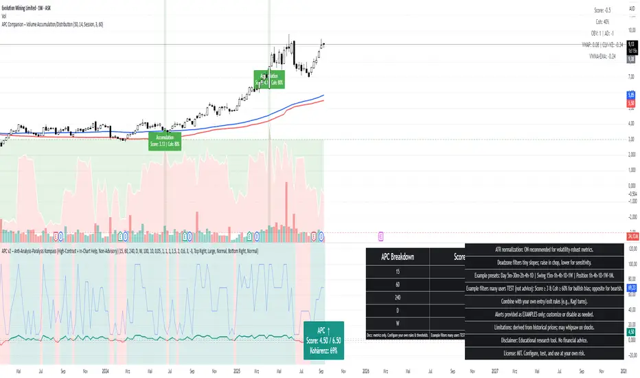
APC Companion – Volume Accumulation/DistributionIndicator Description (TradingView – Open Source)
APC Companion – Volume Accumulation/Distribution Filter
(Designed to work standalone or together with the APC Compass)
What this indicator does
The APC Companion measures whether markets are under Accumulation (buying pressure) or Distribution (selling pressure) by combining:
Chaikin A/D slope – volume flow into price moves
On-Balance Volume momentum – confirms trend strength
VWAP spread – price vs. fair value by traded volume
CLV × Volume Z-Score – detects intrabar absorption / selling pressure
VWMA vs. EMA100 – confirms whether weighted volume supports price action
The result is a single Acc/Dist Score (−5 … +5) and a Coherence % showing how many signals agree.
How to interpret
Score ≥ +3 & Coherence ≥ 60% → Accumulation (green) → market supported by buyers
Score ≤ −3 & Coherence ≥ 60% → Distribution (red) → market pressured by sellers
Anything in between = neutral (no strong bias)
Using with APC Compass
Long trades: Only take Compass Long signals when Companion shows Accumulation.
Short trades: Only take Compass Short signals when Companion shows Distribution.
Neutral Companion: Skip or reduce size if there is no confirmation.
This filter greatly reduces false signals and improves trade quality.
Best practice
Swing trading: 4H / 1D charts, lenZ 40–80, lenSlope 14–20
Intraday: 5m–30m charts, lenZ 20–30, lenSlope 10–14
Position sizing: Increase with higher Coherence %, reduce when below 60%
Exits: Reduce or close if Score drops back to neutral or flips opposite
Disclaimer
This script is published open source for educational purposes only.
It is not financial advice. Test thoroughly before using in live trading.
Weekly Fibonacci Pivot Levelsthis indicator in simple ways, draw the weekly fibo zones based on calculations
weekly zones are drawn automatically based on previous week, and are updated once a new week is opened
you can use it the way you like or adapt to your trading strategy
i really use it at extremes and when a divergence is occurring in these zones

Weekly ReboundWeekly Rebound analyzes weekly setups where price is below the EMA200 median (P50) and forms a red→green reversal.
It measures the maximum rebound (%) within 24 weeks and shows historical stats (average, median, P25–P75, time to peak).
